A New Family of Unitary Space-Time Codes with a Fast Parallel Sphere Decoder Algorithm

Abstract

In this paper we propose a new design criterion and a new class of unitary signal constellations for differential space-time modulation for multiple-antenna systems over Rayleigh flat-fading channels with unknown fading coefficients. Extensive simulations show that the new codes have significantly better performance than existing codes. We have compared the performance of our codes with differential detection schemes using orthogonal design, Cayley differential codes, fixed-point-free group codes and product of groups and for the same bit error rate, our codes allow smaller signal to noise ratio by as much as 10 dB.

The design of the new codes is accomplished in a systematic way through the optimization of a performance index that closely describes the bit error rate as a function of the signal to noise ratio. The new performance index is computationally simple and we have derived analytical expressions for its gradient with respect to constellation parameters.

Decoding of the proposed constellations is reduced to a set of one-dimensional closest point problems that we solve using parallel sphere decoder algorithms. This decoding strategy can also improve efficiency of existing codes.

1 Introduction

Recently there have been extensive research interests in wireless communication links with multiple transmitter antennas. For the Rayleigh-fading channel models, information-theoretic analysis has shown that the capacity of a communication link with multiple transmitter antennas can substantially exceed that of a single-antenna link [10], [11], [31], [46], [55]. Several coding and modulation schemes have also been proposed to exploit the potential increase in the capacity through space diversity. For the coherent multiple-antenna channel, several transmit diversity methods and code construction have been presented in [3], [42], [43] and the references therein (see, e.g., [7], [12], [14], [17], [34]–[36], [38], [47], [50]–[53]). In particular, Tarokh, Seshadri, and Calderbank [42] proposed space-time codes which combine signal processing at the receiver with coding techniques appropriate to multiple transmitter antennas. Alamouti [3] discovered a remarkable transmitter diversity scheme for two transmitter antennas, which was later generalized by Tarokh et al. [43] as a framework for space-time block codes. Motivated by the fact that, in many situations, channel state information may not be available to the receiver, Hochwald and Marzetta [21] proposed a general signaling scheme, called unitary space-time modulation, and showed that this scheme can achieve a high ratio of channel capacity in combination with channel coding. The design of unitary space-time constellations was investigated in [1], [18] and [19]. More recently, differential modulation and code construction methods for multiple transmit antennas have been proposed by Hochwald et al. [20], Hughes [22], Tarokh et al. [25, 44] and some other researchers (see, e.g., [4], [16], [23], [24], [27], [30], [32], [40, 41], [49], [54]).

We investigate the encoding and decoding issues for the differential unitary space-time modulation scheme independently proposed by Hochwald and Sweldens in [20] and Hughes in [22]. A number of unitary space-time codes have been proposed aimed at achieving high performance, low encoding and decoding complexity. Among these, we recall the orthogonal design (see, [25, 44]), cyclic group codes [20, 22], Caley differential (CD) codes [16] and the full-diversity codes such as fixed-point-free (FPF) unitary group codes $G_{m,r}$, non-group codes $S_{m,s}$ and products of cyclic groups [39]. Orthogonal design has extremely low decoding complexity; unfortunately, the performance degrades significantly when the number of receiver antennas is more than one or the data rate is high. Caley differential codes and the full-diversity codes outperform orthogonal designs in many cases, while the decoding complexity is much higher than that of orthogonal designs. The main idea of decoding the full-diversity codes and Caley differential codes is to formulate the decoding problem as a closest point problem and then solve it by existing methods such as “LLL” lattice algorithm and sphere decoder algorithm. The decoding complexity depends critically on the dimension of the underlying closest point problem.

In this paper we develop a new paradigm for the design of high performance, low encoding and decoding complexity, unitary space-time codes. Similar to the full-diversity codes $G_{m,r}$, $S_{m,s}$ and products of cyclic groups, our proposed constellations also use diagonal matrices as the kernel for fast decoding purpose. However, in sharp contrast to those existing codes which are parameterized by special integers, our constellations are defined by real-valued parameters and are not restricted to have full diversity or group structure. Consequently, unitary space-time code with our proposed structure exists for any combination of antennas and constellation size.

We define a code performance index that describes the bit error rate as a function of the signal to noise ratio. The index is simple to evaluate yet highly accurate in the normal signal to noise ratio (SNR) region. As a result, it is possible to bring all the power of non-linear programming into the code design. We have developed a complete gradient descent algorithm to design constellations that are optimal with respect to the bit error rate. It should be noted that the idea of code design by gradient-based optimization for non-coherent MIMO channels was proposed before in [1] and [16]. A systematic design of unitary constellation based on random search has been proposed in [19]. Our approach differs from the previous works in the design criterion, the structure of signal constellations, and the decoding method. We attempt to apply gradient descent techniques to directly minimize the bit error rate over signal constellations which allow for efficient decoding algorithms.

Exploiting the special structure of our proposed constellations, the decoding problem is reduced to one-dimensional closest point problems which can be efficiently solved in parallel. Based on that strategy, we have developed parallel sphere decoder algorithms which can also be applied to improve decoding efficiency of existing codes.

Based on the new structure and using the optimal design techniques, we have obtained constellations which significantly outperform existing ones. For example, with spectral efficiency $R=6$ bits per channel use, we have found a constellation which improves upon orthogonal design by about $10$ dB at block error rate $6\times 10^{-2}$ when using two transmitter and receiver antennas. With the same configuration, the corresponding improvement upon Caley differential code is about $9$ dB.

In the rest of this section we establish the notation and describe the channel model. Section 2 introduces the structure of the new constellations and develops the optimization procedure for their design. Specifically, we introduce the performance index that converts constellation design into a minimization problem amenable to steepest descent techniques and derive simple expressions for the computation of its gradient. Section 3 develops a parallel sphere decoder algorithm that can also be applied to improve existing codes. Section 4 presents results of the performed simulations. Section 5 summarizes our findings. Proofs and constellation data are provided in the Appendices.

1.1 Notation

Throughout this paper, we use the following notations.

$\mathbb{R}$ — real number field;

$\mathbb{C}$ — complex number field;

$\mathbb{Z}$ — integer set;

$\lfloor.\rfloor$ — floor function;

$\lceil.\rceil$ — ceiling function;

$\lfloor x\rceil$ — the integer closest to $x$;

${\rm mod}^{*}(x)$ — symmetric modulus operation such that ${\rm mod}^{*}(x)$ has range $[-\frac{x}{2},\frac{x}{2})$;

$\arg(.)$ — phase angle operator taking values in $[-\pi,\;\pi)$;

$\det(.)$ — determinant function;

${\rm tr}(.)$ — trace function;

${\rm diag}([x_{1},\cdots,x_{n}])$ — diagonal matrix with $x_{p}$ at the $p$-th row and the $p$-th column;

$||X||$ — Euclidean norm of vector $X$;

$||X||_{\mathrm{F}}$ — Frobenius norm of matrix $X$;

$[X]_{pq}$ — entry of $X$ at the $p$-th row and $q$-th column;

$\Re(X)$ — real part of $X$;

$\Im(X)$ — imaginary part of $X$;

$X^{\intercal}$ — transpose of $X$;

$X^{\dagger}$ — conjugate transpose of $X$;

${\rm abs}(X)$ — the matrix obtained by replacing each entry of $X$ with its modulus;

$\mathcal{CN}(0,1)$ — complex random variable with zero mean and variance one.

$\nabla g({\bf x})$ — gradient of function $g({\bf x})$.

1.2 Channel Model

Consider a communication link with $M$ transmitter and $N$ receiver antennas operating in a Rayleigh flat-fading channel, which can be described by the following channel model [20]

$$X_{\tau}=\sqrt{\rho}S_{\tau}H_{\tau}+W_{\tau}$$

where $\tau$ is the index of time frame, $H_{\tau}\in\mathbb{C}^{M\times N}$ is the channel matrix with $\mathcal{CN}(0,1)$ entries and is unknown to the receiver and the transmitter, $S_{\tau}\in\mathbb{C}^{M\times M}$ is the transmitted signal, $X_{\tau}\in\mathbb{C}^{M\times N}$ is the received signal, $W_{\tau}\in\mathbb{C}^{M\times N}$ is Gaussian noise with $\mathcal{CN}(0,1)$ entries, and $\rho$ is the expected SNR at each receiver antenna. It should be noted that the channel matrix $H_{\tau}$ has been normalized so that the SNR is not dependent on the number of transmitter antennas. It is assumed that the channel matrix is approximately constant within two consecutive time frames, i.e., $H_{\tau}\approx H_{\tau-1}$. However, for the $\tau$-th and the $\iota$-th time frames that are not consecutive, $H_{\tau}$ and $H_{\iota}$ are mutually independent and thus their realizations can be significantly different. The transmitted signals are determined by the following fundamental differential transmitter equations [20]

$$S_{0}=I_{M\times M},\;\;\;\;S_{\tau}=V_{\tau}S_{\tau-1},\;\tau=1,2,\cdots$$

where $V_{\tau}\in\mathbb{C}^{M\times M}$ is a unitary matrix picked from signal constellation $\mathcal{V}$. It is shown in [20, 21, 22] that the maximum-likelihood (ML) detection is to minimize

$$||X_{\tau}-V_{\ell}X_{\tau-1}||_{\mathrm{F}}^{2}$$

among all possible $V_{\ell}\in\mathcal{V}$. The Chernoff bound of pair-wise probability of mistaking $V_{\ell}$ for $V_{\ell^{{}^{\prime}}}$ or vice versa is given by [21]

$$P(V_{\ell},\;V_{\ell^{{}^{\prime}}})=\frac{1}{2}\prod_{m=1}^{M}\left[1+\frac{\rho^{2}\sigma_{m}^{2}}{4(1+2\rho)}\right]^{-N}$$ (1)

where $\sigma_{m}$ is the $m$-th singular value of $V_{\ell}-V_{\ell^{{}^{\prime}}}$.

2 A New Constellation Design Approach

The new code design paradigm that we propose uses diagonal matrices, as in [39], to simplify the decoding process. Our approach is similar to [1] and [16] in the spirit of relaxing the code structures from strict structures such as orthogonal or diagonal structure, parameterizing the codes, and employing the powerful gradient-based optimization to find the best codes. A significant new feature is the ability to formulate the design as a non-linear programming problem that directly minimizes the bit error rate. In the following, we begin our presentation by introducing new codes that are functions of real-valued variables and do not require full diversity. Then we introduce the cost function and derive expressions for its gradient that are used in a steepest descent design algorithm.

2.1 Constellation Structure

In this section, we introduce a new class of unitary space-time codes which can be efficiently encoded and decoded. Similar to the full-diversity codes such as FPF code $G_{m,r}$, non-group code $S_{m,s}$ and products of cyclic groups [39], our proposed constellation also involves diagonal matrices for fast decoding purpose. However, in sharp contrast to those full-diversity codes which are parameterized by particular integers, our proposed constellations are determined by continuous parameters and are not restricted to have full diversity or group structure. Consequently, unitary space-time code with our proposed structure exists for any combination of antennas and constellation size.

Let $b\geq 0$ be an integer and let $L$ be a power of $2$. We construct a constellation $\mathcal{V}$ with $\mathscr{L}=2^{b}L$ signal matrices as follows.

For $q=0,1,\;\cdots,\;2^{b}-1$, define

$$\Lambda_{q}\stackrel{{\scriptstyle\mathrm{def}}}{{=}}{\rm diag}\left(\left[\exp\left(\frac{i2\pi\lambda_{q,1}}{L}\right),\;\cdots,\;\exp\left(\frac{i2\pi\lambda_{q,M}}{L}\right)\right]\right),$$

where $\lambda_{q,1}=1$ and $\lambda_{q,m}\in[0,\;L),\;\;m=2,\cdots,M$ are real-valued parameters. Let $A_{0}=B_{0}=I$ and $A_{q},\;B_{q},\;\;q=1,\;\cdots,\;2^{b}-1$ be unitary matrices. Then the constellation is given by

$$\mathcal{V}=\{A_{q}\Lambda_{q}^{\ell}B_{q}\;\;|\;\;\ell=0,\;1,\;\cdots,\;L-1;\;\;q=0,1,\;\cdots,\;2^{b}-1\}.$$

We note that the constellation design problem is to find $\lambda_{q,m}$ and $A_{q},\;\;B_{q}$ so that the bit error rate is minimized. We shall show that this problem can be solved efficiently.

For the purpose of comparing our constellations with existing ones, we note that the spectral efficiency of our proposed constellation is

$$R=\frac{\log_{2}(\mathscr{L})}{M}=\frac{b+\log_{2}(L)}{M}.$$

It should be noted that, for the special case $b=0$, the signal constellation reduces to

$$\{\Lambda^{\ell}\;|\;\ell=0,1,\cdots,L-1\}$$

where

$$\Lambda={\rm diag}\left(\left[\exp\left(\frac{i2\pi\lambda_{1}}{L}\right),\;\cdots,\;\exp\left(\frac{i2\pi\lambda_{M}}{L}\right)\right]\right)$$

with $\lambda_{1}=1$ and continuous parameters $\lambda_{m}\in[0,\;L),\;\;m=2,\cdots,M$. We refer to such constellation as a continuous diagonal code. Obviously, it is a generalization of cyclic group code.

In general, with fixed constellation size $\mathscr{L}$, the performance may be significantly improved by increasing the number of blocks (i.e., $\frac{\mathscr{L}}{L}$). Interestingly, we shall show that the decoding complexity increases slightly with respect to the number of blocks. This property can be attributed to our parallel sphere decoder algorithms, discussed in Section 3.

2.2 Design Performance Index

Efficient constellation design is a challenging task due to the large number of parameters. In addition to the structure of the constellations, the design criterion is also critical for the achievable bit error rate performance. One of the widely used criterion is to use the diversity product as the performance measure of a constellation. The design objective is to maximize the diversity product over a class of constellations that have full diversity (see, e.g., [20] [27], [39] and the references therein). The drawbacks of the conventional design criterion are the following: First, the diversity product is essentially a worst-case measure. In many situations, the overall performance of a constellation is not governed by the behavior of extreme signal matrices. As can be seen from our experimental results in Section 4, it is not uncommon to have constellations with zero diversity product significantly outperforming constellations with the largest diversity product previously known. Second, the measure diversity product is derived by an asymptotic argument. The idea is that, as the SNR tends to infinity, the Chernoff bound of the pair-wise error probability is dominated by the determinant of the difference of the pair of unitary matrices. Such asymptotic argument is not flawless. It is not clear how large the value of SNR can be approximated as infinity so that no significant inaccuracy will be introduced in the evaluation of the block (or bit) error rate.

In light of the limitations of the worst-case and asymptotic design criterion, we have established a new design criterion which incorporates the bits assignment in the optimization of constellations. Instead of using a worst-case criterion such as diversity product [20], we introduce a performance index that measures directly the bit error rate as a function of the signal to noise ratio. The index is analytically tractable and possesses simple analytical expressions for its gradient. Motivated by the fact that, for large constellation size, the bit error rate may not be well governed by the block error rate, we shall also incorporate the bit assignments in the process of constellation optimization. In particular we propose the cost function

$$J=\int_{\rho_{1}}^{\rho_{2}}\log_{10}P_{\mathrm{bit}}(\rho)\;d\log_{10}(\rho)$$

where $P_{\mathrm{bit}}(\rho)$ is the union bound of bit error probability and $[\rho_{1},\rho_{2}]$ is the interval of SNR of practical interests. We shall show that this cost function can be well approximated by a very simple analytical expression.

From numerous simulation results published in the literature, we notice that, on a log scale, the bit error rate is an almost linear function of the SNR. Such phenomenon can be illustrated by making use of the Chernoff bound (1). For large SNR, the Chernoff bound $P(V_{\ell},V_{\ell^{{}^{\prime}}})$ of pair-wise error probability can be approximated by

$$P(V_{\ell},V_{\ell^{{}^{\prime}}}) \approx \frac{1}{2}\rho^{-MN}\left(\prod_{m=1}^{M}\frac{\sigma_{m}^{2}}{8}\right)^{-N}$$

$$= \frac{1}{2}\rho^{-MN}\left(\frac{\det(V_{\ell}-V_{\ell^{{}^{\prime}}})}{8}\right)^{-N}.$$

Since such approximation is tight for most combinations $(\ell,\ell^{\prime})$ and $V_{\ell}$ is assumed to be equally likely for all $\ell$, the union bound of the bit error rate is well approximated by

$$P_{\mathrm{bit}}(\rho)\approx\rho^{-MN}\;\frac{\sum_{\ell\neq\ell^{\prime}}\;d^{\mathrm{H}}(\ell,\ell^{\prime})\left(\frac{\det(V_{\ell}-V_{\ell^{{}^{\prime}}})}{8}\right)^{-N}}{2\mathscr{L}\log_{2}\mathscr{L}}$$

where $d^{\mathrm{H}}(\ell,\ell^{\prime})$ denotes the Hamming distance of bits assigned to $V_{\ell}$ and $V_{\ell^{\prime}}$. Applying logarithm operation gives

$$\log_{10}P_{\mathrm{bit}}(\rho)$$

$$\approx -\frac{MN}{10}\;10\log_{10}(\rho)$$

$$+\log_{10}\left(\frac{\sum_{\ell\neq\ell^{\prime}}\;d^{\mathrm{H}}(\ell,\ell^{\prime})\;\left(\frac{\det(V_{\ell}-V_{\ell^{\prime}})}{8}\right)^{-N}}{2\mathscr{L}\log_{2}\mathscr{L}}\right).$$

Figure 1 displays the actual cost function and the proposed approximation. For completeness we mention that the block error rate admits a similar approximation.

Due to the excellent linearity of the performance curve in the logarithm scale, the cost function can be well approximated by

$$\zeta(\mathcal{V}) \stackrel{{\scriptstyle\mathrm{def}}}{{=}} [\log_{10}P_{\mathrm{bit}}(\rho_{2})+\log_{10}P_{\mathrm{bit}}(\rho_{1})]$$

$$\times\;[\log_{10}(\rho_{2})-\log_{10}(\rho_{1})].$$

We propose to design constellations that minimize the index $\zeta(\mathcal{V})$.

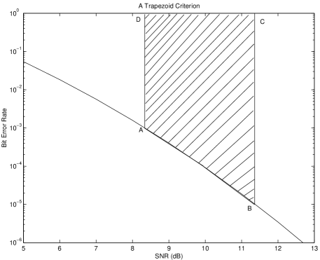
Figure 1: The area of trapezoid ABCD, or equivalently $-\zeta(\mathcal{V})$, reflects the quality of constellation $\mathcal{V}$.

In practice, we can choose $\rho_{1}$ and $\rho_{2}$ based on the performance of the best cyclic group codes previously known. More specifically, $\rho_{1}$ and $\rho_{2}$ can be selected so that two typical levels of bit error rate are respectively guaranteed. For example, we can find $\rho_{1}$ and $\rho_{2}$ such that

$$\log_{10}P_{\mathrm{bit}}(\rho_{1})=10^{-3},\;\;\;\log_{10}P_{\mathrm{bit}}(\rho_{2})=10^{-5}$$

by a bisection method for an existing cyclic group code. When $\rho_{1}$ and $\rho_{2}$ have been found, the criterion measure $\zeta(\mathcal{V})$ is SNR independent. Most importantly, the gradient of $\zeta(\mathcal{V})$ with respect to the constellation parameters can be computed efficiently and thus allows for a gradient descent method for constellation design. The optimization technique is described in the next section.

2.3 Constellation Optimization

In this section, we perform a global optimization to find unitary constellations of good performance. Our strategy is to first choose the bit assignment and then search the code parameters to minimize the bit error rate. The advantage of this strategy is that the objective function $\zeta(\mathcal{V})$ is a differentiable function and is amenable for gradient-based optimization. On the other hand, if we first search the good code matrices and then try to find the best bit assignment, we need to solve a combinatorial optimization problem. In general, such combinatorial problem is not tractable for gradient-based optimization techniques because the objective function is not continuous. The only method for solving such combinatorial problem is the exhaustive random search. Unfortunately, for large constellations, the searching can be extremely inefficient.

2.3.1 Parameterization of Unitary Matrix

In order to develop a gradient-based method for the minimization of the performance measure $\zeta(\mathcal{V})$, the first step is to choose a suitable parameterization for unitary matrices. The application of unitary matrices parameterization [33] in signal constellation design has been pioneered by [1]. We adopt such idea of using parameterized unitary code matrices. In general, a $M\times M$ unitary matrix $U$ can be determined by a set of $M^{2}$ parameters $\Theta$ defined as follows:

$$\phi_{pq}\in\left[-\frac{\pi}{2},\frac{\pi}{2}\right],\qquad 1\leq p<q\leq M-1;$$

$$\phi_{pM}\in[-\pi,\pi),\qquad 1\leq p\leq M-1;$$

$$\nu_{pq}\in\left[-\frac{\pi}{2},\frac{\pi}{2}\right],\qquad 1\leq p<q\leq M;$$

$$\theta_{k}\in\left[-\frac{\pi}{2},\frac{\pi}{2}\right],\qquad k=1,\cdots,M-1;$$

$$\theta_{M}\in[-\pi,\pi).$$

More specifically, let $U^{p,q}(\phi_{pq},\nu_{pq})$ denote a $(M-p+1)$-dimensional unitary matrix such that

$$[U^{p,q}]_{jk}$$

$$= \left\{\begin{array}[]{ll}1,&{\rm if}\;j=k\;{\rm and}\;j\notin\{1,q-p+1\}\\ \cos(\phi_{pq}),&{\rm if}\;j=k\;{\rm and}\;j\in\{1,q-p+1\}\\ -\sin(\phi_{pq})e^{-i\nu_{pq}},&{\rm if}\;j=1\;{\rm and}\;k=q-p+1\\ \sin(\phi_{pq})e^{i\nu_{pq}},&{\rm if}\;k=1\;{\rm and}\;j=q-p+1\\ 0,&{\rm otherwise}\end{array}\right.$$

and let

$$\digamma^{r}=U^{r,r+1}\;U^{r,r+2}\;\cdots\;U^{r,M},$$

then, any unitary matrix $U(\Theta)$ can be represented as

$$U=\mathscr{U}^{M-1}\;\digamma^{1}$$

where

$$\mathscr{U}^{1}=\left[\begin{array}[]{ll}\exp(i\theta_{M-1})&0\\ 0&\exp(i\theta_{M})\end{array}\right]$$

and

$$\mathscr{U}^{k+1}=\left[\begin{array}[]{ll}\exp(i\theta_{M-k-1})&0\\ 0&\mathscr{U}^{k}\;\digamma^{M-k}\end{array}\right]$$

for $k=1,\cdots,M-2$.

2.3.2 Gradient Method

Here we develop explicit expressions for the gradient of the performance measure $\zeta(\mathcal{V})$. For the computation of $\zeta(\mathcal{V})$ we need to evaluate the union bound of the bit error rate, which depends on the bit assignment. With regard to the bit assignment, our intuition is that, if we first search the good code matrices and then try to find the best bit pattern – code matrix assignment, we need to cope with a combinatorial optimization problem. Such combinatorial problem is generally not tractable for gradient-based optimization techniques because the objective function is not differentiable. The available method for solving such combinatorial problem will be random search. Unfortunately, for large constellations, the searching can be extremely difficult. In our design, we shall first fix the bit assignment and then search the code parameters to minimize the bit error rate. In this way, the objective function is a differentiable function and is amenable for gradient-based optimization techniques.

For simplicity, we use the binary-to-decimal conversion mapping scheme. In such a scheme, a block of $b+\log_{2}(L)$ bits is mapped into a signal matrix $A_{q}\Lambda_{q}^{\ell}B_{q}$ such that the first $b$ bits are the binary representation of the block index $q$ and the remaining bits are the binary representation of the diagonal index $\ell$. Let $d^{\mathrm{H}}(p,q,\ell,\ell^{{}^{\prime}})$ denote the Hamming distance between the bits respectively assigned to signal matrices $A_{p}\Lambda_{p}^{\ell}B_{p}$ and $A_{q}\Lambda_{q}^{\ell^{{}^{\prime}}}B_{q}$. The union bound of the bit error probability is then given by

$$P_{\mathrm{bit}}=\frac{2}{2^{b}\;L\;[b+\log_{2}(L)]}\left(\widehat{\mathcal{P}}+\widetilde{\mathcal{P}}\right)$$ (3)

where

$$\widehat{\mathcal{P}}=\sum_{p=0}^{2^{b}-1}\;\sum_{\ell=0}^{L-2}\;\sum_{\ell^{{}^{\prime}}=\ell+1}^{L-1}d^{\mathrm{H}}(p,p,\ell,\ell^{{}^{\prime}})\;P(\Lambda_{p}^{\ell},\;\Lambda_{p}^{\ell^{{}^{\prime}}})$$

and

$$\widetilde{\mathcal{P}}$$

$$= \sum_{p=0}^{2^{b}-2}\sum_{q=p+1}^{2^{b}-1}\sum_{\ell=0}^{L-1}\sum_{\ell^{{}^{\prime}}=0}^{L-1}d^{\mathrm{H}}(p,q,\ell,\ell^{{}^{\prime}})P(A_{p}\Lambda_{p}^{\ell}B_{p},A_{q}\Lambda_{q}^{\ell^{{}^{\prime}}}B_{q})$$

It can be seen that, using (3) to compute $P_{\mathrm{bit}}$, the number of pair-wise error probabilities to be evaluated is

$$2^{b-1}L(L-1)+2^{b-1}(2^{b}-1)L^{2}.$$

The problem can still be solved using steepest descent method for small to moderate $L$. However, the computational complexity may be high for large $L$. For proof of concept, we focus here on the special case of $\Lambda_{q}=\Lambda,\;\;A_{q}=I$ for $q=0,\cdots,2^{b}-1$, where, exploiting the special structure of the constellation, the number of pair-wise error probabilities to be computed can be substantially reduced to

$$(L-1)+2^{b-1}(2^{b}-1)(2L-1).$$

For this case, we have

Theorem 1

Let $d^{\mathrm{H}}(p,q)$ denote the Hamming distance between the binary representation of integers $p$ and $q$. Define

$$w(k)=\sum_{\ell=0}^{L-k-1}d^{\mathrm{H}}(\ell+k,\;\ell),\;\;\;\;k=0,1,\cdots,L-1.$$

Then

$$P_{\mathrm{bit}}=\frac{2}{L[b+\log_{2}(L)]}\;\left[\mathcal{P}^{\prime}+\sum_{k=1}^{L-1}w(k)\;P(I,\Lambda^{k})\right]$$

where

$$\mathcal{P}^{\prime}=\frac{1}{2^{b}}\sum_{p=0}^{2^{b}-2}\sum_{q=p+1}^{2^{b}-1}\sum_{k=-L+1}^{L-1}[w(|k|)+d^{\mathrm{H}}(p,q)]P(B_{p},\Lambda^{k}B_{q}).$$

See Appendix A for a proof. It should be noted that, to reduce computation, $w(k)$ can be pre-computed and saved as a lookup table.

In order to use gradient descent method to minimize $\zeta(\mathcal{V})$, we need to find the fastest descent direction at every step of searching. Following the procedure in [1], we update $B_{p}$ as $B_{p}U(\Theta)$. In the sequel, we shall show that the computation of the gradient of performance measure $\zeta(\mathcal{V})$ reduces to the computation of: (i) the partial derivatives of functions of the form $P(U(\Theta),\Phi)$ with respect to $\Theta$ at $\Theta=0$ (i.e., all elements of $\Theta$ are zero); (ii) the partial derivatives of functions of the form $P(\Lambda^{\ell},\Phi)$ with respect to $\Lambda={\rm diag}([e^{2\pi i\lambda_{1}/L},\cdots,e^{2\pi i\lambda_{M}/L}])$ at $\Lambda=I$ (i.e., $\lambda_{m}=0,\;m=1,\cdots,M$).

We have derived surprisingly simple formulas for computing pair-wise error probabilities and the related partial derivatives.

Theorem 2

Let $U(\Theta)$ be unitary matrix parameterized by $\Theta$. Let $\Phi$ be a unitary matrix. Let

$$\alpha=\frac{4(1+2\rho)}{\rho^{2}},\quad\mathcal{Q}=[(\alpha+2)I-\Phi-\Phi^{\dagger}]^{-1}\Phi$$

and

$$\Lambda={\rm diag}([e^{2\pi i\lambda_{1}/L},\cdots,e^{2\pi i\lambda_{M}/L}]).$$

Then

$$P(I,\Phi)=\frac{\alpha^{MN}}{2\left(\det[(\alpha+2)I-\Phi-\Phi^{\dagger}]\right)^{N}},$$ (4)

$${\left.\frac{\partial P(U,\Phi)}{\partial\phi_{pq}}\right|}_{\Theta=0}=2NP(I,\Phi)\;\Re([\mathcal{Q}]_{qp}-[\mathcal{Q}]_{pq}),\qquad$$ (5)

$${\left.\frac{\partial P(U,\Phi)}{\partial\theta_{k}}\right|}_{\Theta=0}=2NP(I,\Phi)\;\Im([\mathcal{Q}]_{kk}),$$ (6)

$${\left.\frac{\partial P(U,\Phi)}{\partial\nu_{pq}}\right|}_{\Theta=0}=0,$$ (7)

$${\left.\frac{\partial P(\Lambda^{\ell},\Phi)}{\partial\lambda_{m}}\right|}_{\Lambda=I}=\frac{4\pi N\ell}{L}P(I,\Phi)\;\Im([\mathcal{Q}]_{mm}).$$ (8)

See Appendix B for a proof. At the first glance, it is not clear how Theorem 2 can be applied to the optimization of code matrices. From the expression of our performance metric $\zeta(\mathcal{V})$, it can be seen that it suffices to compute the gradients of $P_{\mathrm{bit}}(\rho_{1})$ and $P_{\mathrm{bit}}(\rho_{2})$ with respect to code parameters. From (3), we can see that, since the bits assignment is fixed, it suffices to compute the gradient of $P(\Lambda_{p}^{\ell},\;\Lambda_{p}^{\ell^{{}^{\prime}}})$ and $P(A_{p}\Lambda_{p}^{\ell}B_{p},\;A_{q}\Lambda_{q}^{\ell^{{}^{\prime}}}B_{q})$ with respect to code parameters for all combinations of $p$ and $q$. Note that the first quantity can be viewed as a special case of the second. Hence, we focus on the second quantity $P(A_{p}\Lambda_{p}^{\ell}B_{p},\;A_{q}\Lambda_{q}^{\ell^{{}^{\prime}}}B_{q})$. We first consider how to update the matrix $B_{p}$. In order to apply the gradient descent method to minimize the performance metric, we need the partial derivatives of the function $P(A_{p}\Lambda_{p}^{\ell}B_{p},\;A_{q}\Lambda_{q}^{\ell^{{}^{\prime}}}B_{q})$ with respect to the parameters of $B_{p}$. It can be seen from the complexity of the function $P(.,.)$ and the parameterization of $B_{p}$ that the direct computation of the partial derivatives can be extremely difficult. Observing that, at every step, $B_{p}$ is to be updated as $\widehat{B}_{p}$ which is also a unitary matrix. Hence, there must be an unitary matrix $U(\Theta)$ such that $\widehat{B}_{p}=B_{p}U(\Theta)$. This means that we can update the unitary matrices in a multiplicative way. As mentioned earlier, this method of updating unitary matrices was proposed in [1]. In the same sprit with that of the conventional steepest-descent minimization, to make $P(A_{p}\Lambda_{p}^{\ell}B_{p},\;A_{q}\Lambda_{q}^{\ell^{{}^{\prime}}}B_{q})$ descent in a fastest way as $B_{p}$ is varying to a new matrix, we can choose $U(\Theta)$ based on the partial derivatives of $P(A_{p}\Lambda_{p}^{\ell}B_{p}U(\Theta),\;A_{q}\Lambda_{q}^{\ell^{{}^{\prime}}}B_{q})$ with respect to $\Theta$ at $\Theta=0$. The computation of the derivatives can be accomplished by applying Theorem 2 and the following fact:

$P(.,.)$ is invariant under unitary transforms. That is, for any unitary matrices $X$ and $Y$, $P(U_{L}XU_{R},\;Y)=P(X,\;U_{L}^{\dagger}YU_{R}^{\dagger})$ for any unitary matrices $U_{L}$ and $U_{R}$.

To prove this fact, we can use equation (29), which is shown in Appendix B. By (29),

$$P(U_{L}XU_{R},Y)$$

$$= \frac{\alpha^{MN}}{2\left(\det[\alpha I+(U_{L}XU_{R}-Y)(U_{L}XU_{R}-Y)^{{\dagger}}]\right)^{N}}.$$

Observing that

$$(U_{L}XU_{R}-Y)(U_{L}XU_{R}-Y)^{{\dagger}}$$

$$= U_{L}(X-U_{L}^{\dagger}YU_{R}^{\dagger})U_{R}U_{R}^{\dagger}(X-U_{L}^{\dagger}YU_{R}^{\dagger})^{{\dagger}}U_{L}^{\dagger}$$

$$= U_{L}(X-U_{L}^{\dagger}YU_{R}^{\dagger})(X-U_{L}^{\dagger}YU_{R}^{\dagger})^{{\dagger}}U_{L}^{\dagger},$$

we have

$$\alpha I+(U_{L}XU_{R}-Y)(U_{L}XU_{R}-Y)^{{\dagger}}$$

$$= U_{L}\left[\alpha I+(X-U_{L}^{\dagger}YU_{R}^{\dagger})(X-U_{L}^{\dagger}YU_{R}^{\dagger})^{{\dagger}}\right]U_{L}^{\dagger}.$$

Hence

$$\det\left[\alpha I+(U_{L}XU_{R}-Y)(U_{L}XU_{R}-Y)^{{\dagger}}\right]$$

$$= \det(U_{L}U_{L}^{\dagger})\det\left[\alpha I+(X-U_{L}^{\dagger}YU_{R}^{\dagger})(X-U_{L}^{\dagger}YU_{R}^{\dagger})^{{\dagger}}\right]$$

$$= \det\left[\alpha I+(X-U_{L}^{\dagger}YU_{R}^{\dagger})(X-U_{L}^{\dagger}YU_{R}^{\dagger})^{{\dagger}}\right]$$

and

$$P(U_{L}XU_{R},Y)$$

$$= \frac{\alpha^{MN}}{2\left\{\det\left[\alpha I+(X-U_{L}^{\dagger}YU_{R}^{\dagger})(X-U_{L}^{\dagger}YU_{R}^{\dagger})^{{\dagger}}\right]\right\}^{N}}$$

$$= P(X,\;U_{L}^{\dagger}YU_{R}^{\dagger}).$$

This proves the invariant property. An immediate result from such property is

$$P\left(A_{p}\Lambda_{p}^{\ell}B_{p},\;A_{q}\Lambda_{q}^{\ell^{{}^{\prime}}}B_{q}\right)=P\left(I,\;(A_{p}\Lambda_{p}^{\ell}B_{p})^{\dagger}A_{q}\Lambda_{q}^{\ell^{{}^{\prime}}}B_{q}\right),$$

which implies that we can let $\Phi=(A_{p}\Lambda_{p}^{\ell}B_{p})^{\dagger}A_{q}\Lambda_{q}^{\ell^{{}^{\prime}}}B_{q}$ and apply (4) to compute $P(A_{p}\Lambda_{p}^{\ell}B_{p},\;A_{q}\Lambda_{q}^{\ell^{{}^{\prime}}}B_{q})$.

Making use of such property, we have

$$P\left(A_{p}\Lambda_{p}^{\ell}B_{p}U(\Theta),\;A_{q}\Lambda_{q}^{\ell^{{}^{\prime}}}B_{q}\right)$$

$$= P\left(U(\Theta),\;(A_{p}\Lambda_{p}^{\ell}B_{p})^{\dagger}A_{q}\Lambda_{q}^{\ell^{{}^{\prime}}}B_{q}\right).$$

If we identify $(A_{p}\Lambda_{p}^{\ell}B_{p})^{\dagger}A_{q}\Lambda_{q}^{\ell^{{}^{\prime}}}B_{q}$ as $\Phi$, we have

$$P\left(A_{p}\Lambda_{p}^{\ell}B_{p}U(\Theta),\;A_{q}\Lambda_{q}^{\ell^{{}^{\prime}}}B_{q}\right)=P(U(\Theta),\Phi).$$

Hence, the partial derivatives of $P(A_{p}\Lambda_{p}^{\ell}B_{p}U(\Theta),\;A_{q}\Lambda_{q}^{\ell^{{}^{\prime}}}B_{q})$ can be computed by applying Theorem 2.

Similarly, we can update $A_{p}$ as $A_{p}U(\Theta)$ and compute the partial derivatives of

$$P\left(A_{p}U(\Theta)\Lambda_{p}^{\ell}B_{p},\;A_{q}\Lambda_{q}^{\ell^{{}^{\prime}}}B_{q}\right)$$

$$= P\left(U(\Theta),\;A_{p}^{\dagger}A_{q}\Lambda_{q}^{\ell^{{}^{\prime}}}B_{q}(\Lambda_{p}^{\ell}B_{p})^{\dagger}\right)$$

with respect to $\Theta$ at $\Theta=0$. The calculation can be done by identifying $A_{p}^{\dagger}A_{q}\Lambda_{q}^{\ell^{{}^{\prime}}}B_{q}(\Lambda_{p}^{\ell}B_{p})^{\dagger}$ as $\Phi$ and applying Theorem 2.

In the same spirit, we can update $\Lambda_{p}^{\ell}$ as $(\Lambda_{p}\Lambda)^{\ell}$ and compute the partial derivatives of

$$P\left(A_{p}(\Lambda_{p}\Lambda)^{\ell}B_{p},\;A_{q}\Lambda_{q}^{\ell^{{}^{\prime}}}B_{q}\right)$$

$$= P\left(\Lambda^{\ell},\;(A_{p}\Lambda_{p}^{\ell})^{\dagger}A_{q}\Lambda_{q}^{\ell^{{}^{\prime}}}B_{q}B_{p}^{\dagger}\right)$$

with respect to $\Lambda$ at $\Lambda=I$ (i.e., $\lambda_{m}=0,\;m=1,\cdots,M$). This can be accomplished by letting

$$\Phi=(A_{p}\Lambda_{p}^{\ell})^{\dagger}A_{q}\Lambda_{q}^{\ell^{{}^{\prime}}}B_{q}B_{p}^{\dagger}$$

and invoking Theorem 2.

Finally, because of symmetry, we have

$$P\left(A_{p}\Lambda_{p}^{\ell}B_{p},\;A_{q}\Lambda_{q}^{\ell^{{}^{\prime}}}B_{q}\right)=P\left(A_{q}\Lambda_{q}^{\ell^{{}^{\prime}}}B_{q},\;A_{p}\Lambda_{p}^{\ell}B_{p}\right).$$

Hence, we can update matrices $A_{q},\;\Lambda_{q}$ and $B_{q}$ and compute the corresponding partial derivatives by the similar method as that of matrices $A_{p},\;\Lambda_{p}$ and $B_{p}$.

In the gradient-based optimization, we used the standard steepest gradient descent method in [56], with some minor modification to adapt to parameter bounds. In the course of experimenting with the new design paradigm, we have observed that it is beneficial to apply the following searching strategy.

STEP (a). Find the best constellation of diagonal structure $\{\Lambda^{\ell}\;|\;0\leq\ell\leq L-1\}$. This can be done as follows. First, perform random search to find $n$ good initial values of $\Lambda$. Second, for each initial value of $\Lambda$, perform gradient-based optimization. Finally, choose the best one among the $n$ outcomes.

STEP (b). Let $\Lambda$ be found in the first step. Find the best constellation of special structure $\{\Lambda^{\ell}B_{q}\;|\;\ell=0,\cdots,L-1;\;q=0,\cdots,2^{b}-1\}$ by employing gradient descent search over $B_{q}$ while $\Lambda$ is fixed. Here the initial value of $B_{q}$ can be randomly chosen.

STEP (c). Using the code found at the second step as starting point, search $A_{q},\;B_{q}$ and $\Lambda_{q}$ by gradient descent method. Here the initial value of $A_{q}$ can be randomly chosen.

For Steps (a)-(c) in the above strategy, we have adopted the same choice of the step size as that of the algorithm of [56].

3 Fast Decoding

Now that we have efficient constellation design tools, we focus on the all important decoding problem. In this section, we develop efficient algorithms for decoding our proposed new codes. Interestingly, such decoding algorithms are also applicable to existing codes. For ease of presentation, we first focus on the case that the constellation has only one block (i.e., $b=0$) and the receiver is equipped with only one antenna (i.e., $N=1$). Subsequently, we discuss the decoding for the general cases of multiple blocks and multiple receiver antennas (i.e., $b\geq 0$ and $N\geq 1$).

When $b=0$, the constellation reduces to the continuous diagonal code. The signal constellation consists of $L$ diagonal matrices $V_{\ell}=\Lambda^{\ell},\;\;\ell=0,1,\cdots,L-1$. For $N=1$, the received signal $X_{\tau}\in\mathbb{C}^{M\times 1}$ is a complex vector. As described in [5], the ML decoding problem can be reformulated as a problem of minimizing a Euclidean norm as follows:

$$\widehat{z}^{\mathrm{ML}}_{\tau}$$ (9)

$$= \arg\;\min_{\ell}\;||X_{\tau}-V_{\ell}X_{\tau-1}||_{\mathrm{F}}^{2}$$

$$\approx \arg\min_{\ell}\sum_{m=1}^{M}[(C_{m}\lambda_{m}\ell-C_{m}\varphi_{m})\;{\rm mod}^{*}C_{m}L]^{2}$$

where

$$C_{m}=\sqrt{\left|[X_{\tau}]_{m1}\;[X_{\tau-1}]_{m1}\right|},\quad\varphi_{m}=\arg\left(\frac{[X_{\tau}]_{m1}}{[X_{\tau-1}]_{m1}}\right)\frac{L}{2\pi}.$$

It has been demonstrated in [5] that the approximation in (9) is extremely accurate. Therefore, the decoding problem for the case $b=0,\;\;N=1$ has been transformed into the minimization problem of finding

$$\widehat{z}^{\mathrm{eucl}}=\arg\;\min_{\ell}\;\sum_{m=1}^{M}[(C_{m}\lambda_{m}\;\ell-C_{m}\;\varphi_{m})\;{\rm mod}^{*}C_{m}L]^{2}.$$ (10)

In the following sub-sections we develop an efficient algorithm for this minimization problem.

3.1 Lattice Decoding Algorithms

In the special case that $\lambda_{m},\;m=1,\cdots,M$ are integers, the continuous diagonal code reduces to the cyclic group code. In order to decode the cyclic group code, Clarkson et al., [5] developed an approximate solution for the minimization problem (10). The key steps are as follows:

1. Reformulate minimization problem (10) as a lattice closest point problem

   $$\arg\;\min_{y\in\mathbb{Z}^{1\times M}}\;||yG-\xi||$$ (11)

   where $\xi=[\xi_{1},\cdots,\xi_{M}]$ with $\xi_{m}=C_{m}\;\varphi_{m},\;\;m=1,\cdots,M$ and $G$ is a $M\times M$ generator matrix such that

   $$[G]_{pq}=\left\{\begin{array}[]{ll}C_{q}\lambda_{q}&{\rm for}\;p=1\;{\rm and}\;1\leq q\leq M,\\ C_{q}L&{\rm for}\;1<p=q\leq M,\\ 0&{\rm else}.\end{array}\right.$$

2. Apply the “LLL” lattice algorithm [26] to find an approximate solution $\widetilde{y}=[\widetilde{y}_{1},\cdots,\widetilde{y}_{M}]$ for (11). An estimate for $\widehat{z}^{\mathrm{eucl}}$ is taken as $\widetilde{y}_{1}\;{\rm mod}\;L$.

While the “LLL” lattice algorithm approximately solves (11), existing sphere decoder algorithms (see, e.g., [2], [6, 8], [9], [48] and the references therein) can provide an exact solution for (11) and hence improve decoding accuracy. The sphere decoder takes advantage of the lattice structure of the received signals and proceeds as follows: (i) It searches the closest lattice points to the received signal which are enclosed in a sphere centered at the received signal; (ii) each time a lattice point of a smaller norm is found, it reduces the sphere radius accordingly and restart the search until an empty sphere is reached. The choice of initial radius depends on the lattice considered, as well as on the additive noise level. At the heart of the sphere decoder algorithm is the subroutine which serves the purposes of: (a) determining whether a sphere $||y\;G-\xi||^{2}<\gamma^{2}$ with fixed radius $\gamma>0$ is empty; (b) detecting a vector in it otherwise. A Cholesky factorization is performed to find an upper triangular matrix $D$ so that $D^{\intercal}D=GG^{\intercal}$, from which the boundary conditions of the sphere can be derived as

$$z_{k}-\sqrt{\frac{\vartheta_{k}}{t_{kk}}}-\varpi_{k}<y_{k}<\sqrt{\frac{\vartheta_{k}}{t_{kk}}}-\varpi_{k}+z_{k},\;k=M,M-1,\cdots,1$$ (12)

where

$$[z_{1},\cdots,z_{M}]=\xi G^{-1},\;\varpi_{k}=\sum_{j=k+1}^{M}t_{kj}(y_{j}-z_{j}),\;k=1,\cdots,M$$

and

$$\vartheta_{M}=\gamma^{2},\;\;\;\vartheta_{k-1}=\vartheta_{k}-t_{kk}\;(y_{k}-z_{k}+\varpi_{k})^{2},\;\;\;k=2,\cdots,M$$

with $t_{kk}=[D]_{kk}^{2},\;\;k=1,\cdots,M$ and $t_{kj}=\frac{[D]_{kj}}{[D]_{kk}},\;\;1\leq k<j\leq M$ (see, e.g., [9, 48] for details). Clearly, the boundary of $y_{k}$ depends on values of $y_{j},\;\;j=k+1,\cdots,M$. If the set of feasible values of $y_{M}$, denoted by $\mathcal{I}_{M}$, is not empty, then for each member $y_{M}$ of $\mathcal{I}_{M}$ the values of other coordinates needed to be evaluated in the sphere decoder algorithm can be represented as the nodes of a tree starting from $y_{M}$. The following Figure 2 depicts this tree structure. In the tree, the children nodes are generated from the parent nodes in accordance with the boundary equation (12). A path of length $M$ (i.e., consisting of $M$ nodes) corresponds to a vector located in the sphere. When $\mathcal{I}_{M}$ has multiple members, the task of the core subroutine is to search among the multiple trees to determine whether there is a path of length $M$ and identify one if there exists. It should be noted that, in sphere decoding, most of the computational efforts are devoted to the evaluation of paths of length less than $M$.

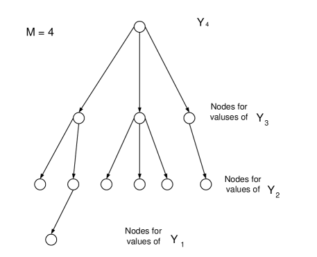
Figure 2: A tree representation of values of coordinates to be investigated for a fixed $y_{M}$.

3.2 Removing the Curse of Dimensionality

In the general case that $\lambda_{m},\;m=1,\cdots,M$ are continuous parameters, the minimization problem in (10) lacks the lattice structure. Hence, existing sphere decoder algorithms and “LLL” lattice algorithm are not applicable. Moreover, even for the special case of cyclic group code, the lattice decoding algorithms described in the last subsection aim to solve a closest point problem of dimension $M$ (the dimension will be expanded to $MN$ when using $N$ receiver antennas). The computational complexity may be too high when the number of transmitter antennas $M$ (or the number of receiver antennas $N$) is large. Therefore, it is crucial to reduce the dimension of the underlying closest point problem by further exploiting the diagonal structure of signal constellation. We achieve the reduction and improve efficiency with a new decoding algorithm, applicable to the general case that $\lambda_{m},\;m=1,\cdots,M$ are continuous parameters. As a critical step to reduce decoding complexity, we will show next that the dimension of the related closest point problem can be reduced to one.

Theorem 3

Define

$$\begin{array}[]{ll}{\mathcal{S}}&=\;\{(y_{1},\cdots,y_{M})\;|\>y_{1}\in\mathbb{Z}\\ &\qquad{\rm and}\;-\frac{L}{2}+\varphi_{1}\leq y_{1}<\frac{L}{2}+\varphi_{1};\\ &\qquad y_{m}=\left\lceil\frac{\varphi_{m}}{L}-(\frac{y_{1}}{L}-\lfloor\frac{y_{1}}{L}\rfloor)\lambda_{m}-\frac{1}{2}\right\rceil-\lfloor\frac{y_{1}}{L}\rfloor\lambda_{m}\\ &\qquad{\rm for}\;\;m=2,\cdots,M\}.\end{array}$$

Suppose that there exists an unique $\widehat{\ell}\in\{0,1,\cdots,L-1\}$ such that

$$\sum_{m=1}^{M}[(C_{m}\lambda_{m}\;\widehat{\ell}-C_{m}\varphi_{m})\;{\rm mod}^{*}C_{m}L]^{2}$$

$$= \min_{\ell}\;\sum_{m=1}^{M}[(C_{m}\lambda_{m}\;\ell-C_{m}\varphi_{m})\;{\rm mod}^{*}C_{m}L]^{2}.$$

Then

$$\widehat{\ell} = \arg\;\min_{\ell}\;\sum_{m=1}^{M}[(C_{m}\lambda_{m}\;\ell-C_{m}\varphi_{m})\;{\rm mod}^{*}C_{m}L]^{2}$$

$$= \widehat{y}_{1}-\left\lfloor\frac{\widehat{y}_{1}}{L}\right\rfloor\;L$$

where $\widehat{y}_{1}$ is first entry of

$$\widehat{y}=[\widehat{y}_{1},\cdots,\widehat{y}_{M}]=\arg\;\min_{y\in\mathcal{S}}||yG-\xi||^{2}.$$

See Appendix C for a proof.

It can be seen from Theorem 3 that $y_{q}$, for $q=2,\cdots,M$, is uniquely determined by $y_{1}$. Hence, finding

$$\arg\;\min_{y\in\mathcal{S}}||yG-\xi||^{2}$$ (13)

is essentially a one-dimensional closest point problem.

Next, by exploiting the special structure of the constellation, we derive extremely simple boundary conditions for the sphere $\left\{y\in\mathcal{S}\;\left|\;||yG-\xi||^{2}<\gamma^{2}\right.\right\}$.

Theorem 4

Let $y=[y_{1},\cdots,y_{M}]\in\mathcal{S}$. Define

$$\mu_{1}=[C_{1}\left(y_{1}-\varphi_{1}\right)]^{2}$$

and

$$\mu_{m}=\mu_{m-1}+[C_{m}\left(Ly_{m}+\lambda_{m}y_{1}-\varphi_{m}\right)]^{2}$$

for $m=2,\cdots,M$. Then $||yG-\xi||^{2}<\gamma^{2}$ if and only if $y_{1}$ is an integer satisfying

$$\varphi_{1}-\frac{\gamma}{C_{1}}<y_{1}<\frac{\gamma}{C_{1}}+\varphi_{1},\;\;\;\;-\frac{L}{2}+\varphi_{1}\leq y_{1}<\frac{L}{2}+\varphi_{1}$$ (14)

and

$$\mu_{m}<\gamma^{2}\;\;{\rm for}\;\;m=2,\cdots,M.$$ (15)

See Appendix D for a proof.

It can be seen that the conditions in (14) determine an interval $\mathcal{I}_{1}$ of feasible values for $y_{1}$. For each value of $y_{1}\in\mathcal{I}_{1}$, we only need to evaluate the simple conditions in (15). This is in sharp contrast to the search over a tree structure described above in the context of sphere decoder.

It should be noted that the sphere decoding algorithm is originally devised to find closest lattice points. In general, our decoding problem is not a problem of searching closest lattice points. However, we can still use the sphere decoding algorithm because the enumeration of interior points of a sphere can be efficiently done as the case of a lattice problem. Moreover, Theorem 4 indicates that the “sphere” can actually be reduced to an “interval” of one dimension.

3.3 Simplified Sphere Decoder

Using the reduction of dimensionality described in the last subsection, we now develop a new decoding algorithm which also applies to continuous diagonal codes, FPF codes $G_{m,r}$, non-group codes $S_{m,s}$ and products of groups. To further enhance efficiency, we adopt the “zigzag” searching strategy originated in [37] and the idea proposed in [8] for avoiding repeated computations.

Obviously, the search for $y_{1}$ can significantly affect the efficiency. Let $\widehat{y}$ denote the vector corresponding to the transmitted signal. Intuitively, for moderate and high SNR, it is more likely for the received signal $\xi$ to be closer to $\widehat{y}\;G$. Since $|y_{1}-\varphi_{1}|<||yG-\xi||$, we should first investigate $y_{1}$ which is closer to $\varphi_{1}$ for a better chance of detecting $\widehat{y}$. Therefore, we shall investigate $y_{1}$ in the following sequence,

$$\lfloor\varphi_{1}\rceil+(-1)^{k}\left\lfloor\frac{k}{2}\right\rfloor,\;\;k=0,1,2,\cdots.$$ (16)

That is, the investigation is started from $\lfloor\varphi_{1}\rceil$ and proceeded in a “zigzag” order in the outward directions (see, e.g., [2], [37]). Note that condition (14) implies

$$-\left\lceil\min\left(\frac{\gamma}{C_{1}},\;\frac{L}{2}\right)\right\rceil\leq y_{1}-\lfloor\varphi_{1}\rceil\leq\left\lceil\min\left(\frac{\gamma}{C_{1}},\;\frac{L}{2}\right)\right\rceil.$$

Hence, it suffices to investigate

$$y_{1}=\lfloor\varphi_{1}\rceil+(-1)^{k}\left\lfloor\frac{k}{2}\right\rfloor,\;\;k=0,1,\cdots,2\left\lceil\min\left(\frac{\gamma}{C_{1}},\;\frac{L}{2}\right)\right\rceil.$$

It is also important to avoid repeated investigation of $y_{1}$. When a value of $y_{1}$ is found to satisfy condition (15), the radius $\gamma$ is reduced as $\sqrt{\mu_{M}}$ and the interval confining $y_{1}$ is consequently shrunk. In this way, the range of $y_{1}$ needed to be investigated is squeezed from outside. To improve efficiency, we use the idea of [8] to ensure that the range of $y_{1}$ needed to be investigated is also squeezed from inside. The idea is based on the following observation:

For a given radius $\gamma$, if a value of $y_{1}$ violates the boundary conditions, then the same value of $y_{1}$ also violates the corresponding boundary conditions after $\gamma$ is reduced.

Therefore, we can keep a record for the values of $y_{1}$ which have been investigated in order to avoid repeated computation. For this purpose, the index variable $k$ in (16) can be used as an indicator for the range of values investigated.

In summary, the decoding algorithm is presented as follows.

STEP 1. Input $\gamma\leftarrow\gamma_{\mathrm{init}}$ where initial radius $\gamma_{\mathrm{init}}$ is chosen based on noise level. Let $k\leftarrow 0$ and $\widetilde{y_{1}}\leftarrow\lfloor\varphi_{1}\rceil$.

STEP 2. Let $k_{\mathrm{max}}\leftarrow 2\left\lceil\min\left(\frac{\gamma}{C_{1}},\;\frac{L}{2}\right)\right\rceil$.

STEP 3. If $k\leq k_{\mathrm{max}}$, let $y_{1}\leftarrow\lfloor\varphi_{1}\rceil+(-1)^{k}\left\lfloor\frac{k}{2}\right\rfloor$ and $k\leftarrow k+1$. Otherwise, let $\gamma\leftarrow\frac{4}{3}\gamma,\;\;\;k\leftarrow 0$ and go to STEP 2.

STEP 4. If condition (15) is violated, go to STEP 3. Otherwise, let $\widetilde{y_{1}}\leftarrow y_{1},\;\;\;\gamma\leftarrow\sqrt{\mu_{M}}$.

STEP 5. Using $\gamma,\;\widetilde{y_{1}}$ and $k$ as input, call subroutine CLOSEST-POINT to find $\widehat{y_{1}}$. Then $\widehat{z}^{\mathrm{eucl}}$ is calculated as $\widehat{z}^{\mathrm{eucl}}=\widehat{y}_{1}-\left\lfloor\frac{\widehat{y}_{1}}{L}\right\rfloor L$. Return $\widehat{z}^{\mathrm{eucl}}$ as the estimate and stop.

The subroutine CLOSEST-POINT is presented as follows.

Function: CLOSEST-POINT

STEP 1. Input $\gamma,\;\widetilde{y_{1}}$ and $k$. Let $\widehat{y_{1}}\leftarrow\widetilde{y_{1}}$.

STEP 2. Let $k_{\mathrm{max}}\leftarrow 2\left\lceil\min\left(\frac{\gamma}{C_{1}},\;\frac{L}{2}\right)\right\rceil$.

STEP 3. If $k\leq k_{\mathrm{max}}$, let $y_{1}\leftarrow\lfloor\varphi_{1}\rceil+(-1)^{k}\left\lfloor\frac{k}{2}\right\rfloor$ and $k\leftarrow k+1$. Otherwise, go to STEP 5.

STEP 4. If condition (15) is satisfied, then let $\widehat{y_{1}}\leftarrow y_{1},\;\;\gamma\leftarrow\sqrt{\mu_{M}}$ and go to STEP 2. Otherwise, go to STEP 3.

STEP 5. Return $\widehat{y_{1}}$ and stop.

It can be seen from STEP 3 that the index $k$ has served the purpose of avoiding repeated investigations. Once a nonempty sphere is detected, no value of $y_{1}$ is investigated more than once among the subsequent smaller spheres.

It should be also noted that, compared to conventional sphere decoder algorithms, many computationally expensive steps have been avoided in our algorithm. For examples, the Cholesky factorization of $GG^{\intercal}$ and the computation of $\xi G^{-1}$ are not needed in our algorithms.

3.4 Sphere Decoding – The General Case

We now discuss the decoding problem for the general case of multiple receiver antennas and multiple block constellation (i.e., $N\geq 1,\;b\geq 0$). Since the ML-decoding is computationally difficult, our goal is to develop a sub-optimal decoding method with low decoding complexity. Note that the ML decoding finds

$$\arg\;\min_{\ell,q}||X_{\tau}-A_{q}\Lambda_{q}^{\ell}B_{q}X_{\tau-1}||_{\mathrm{F}}^{2},$$ (17)

which can be done by obtaining

$$\arg\;\min_{\ell}||X_{\tau}-A_{q}\Lambda_{q}^{\ell}B_{q}X_{\tau-1}||_{\mathrm{F}}^{2}$$ (18)

for $q=0,1,\cdots,2^{b}-1$ and seeking the tuple $(\widehat{q},\widehat{\ell})$ minimizing the Frobenius norm. This method is of sequential nature and has been used in [39] for decoding FPF code $G_{m,r}$, non-group code $S_{m,s}$ and products of groups with the “LLL” lattice algorithm sequentially applied to solve (18).

In the general case the underlying closest point problem is of dimension $MN$ and sequential approaches are inefficient. We use the simplified sphere decoder algorithm developed in the previous subsection and transform the decoding problem into $2^{b}$ one-dimensional closest point problems that can be solved in parallel.

Since the Frobenius norm of a matrix is invariant under unitary transformations, we have

$$||X_{\tau}-A_{q}\Lambda_{q}^{\ell}B_{q}X_{\tau-1}||_{\mathrm{F}}^{2} = ||A_{q}^{\dagger}(X_{\tau}-A_{q}\Lambda_{q}^{\ell}B_{q}X_{\tau-1})||_{\mathrm{F}}^{2}$$

$$= ||A_{q}^{\dagger}X_{\tau}-\Lambda_{q}^{\ell}B_{q}X_{\tau-1}||_{\mathrm{F}}^{2}.$$

By a similar method as that of [5], we can show that

$$||A_{q}^{\dagger}X_{\tau}-\Lambda_{q}^{\ell}B_{q}X_{\tau-1}||_{\mathrm{F}}^{2}$$

$$= \sum_{n=1}^{N}\sum_{m=1}^{M}\left|[A_{q}^{\dagger}X_{\tau}]_{mn}-e^{i2\pi\lambda_{q,m}\ell/L}\;[B_{q}X_{\tau-1}]_{mn}\right|^{2}$$

$$= ||X_{\tau}||_{\mathrm{F}}^{2}+||X_{\tau-1}||_{\mathrm{F}}^{2}$$

$$-2\sum_{n=1}^{N}\sum_{m=1}^{M}C_{m,n}^{2}\cos([(\lambda_{q,m}\;\ell-\varphi_{m,n})\;{\rm mod}^{*}L]2\pi/L)$$

$$\approx ||X_{\tau}||_{\mathrm{F}}^{2}+||X_{\tau-1}||_{\mathrm{F}}^{2}-2\sum_{n=1}^{N}\sum_{m=1}^{M}C_{m,n}^{2}$$

$$+\sum_{n=1}^{N}\sum_{m=1}^{M}C_{m,n}^{2}([(\lambda_{q,m}\;\ell-\varphi_{m,n})\;{\rm mod}^{*}L]2\pi/L)^{2}$$

$$= \frac{4\pi^{2}}{L^{2}}\Delta_{q}+\frac{4\pi^{2}}{L^{2}}\times$$

$$\sum_{n=1}^{N}\sum_{m=1}^{M}[(C_{m,n}\lambda_{q,m}\ell-C_{m,n}\varphi_{m,n})\;{\rm mod}^{*}C_{m,n}L]^{2}$$

where

$$C_{m,n}=\sqrt{\left|[A_{q}^{\dagger}X_{\tau}]_{mn}\;[B_{q}X_{\tau-1}]_{mn}\right|},$$

$$\varphi_{m,n}=\arg\left(\frac{[A_{q}^{\dagger}X_{\tau}]_{mn}}{[B_{q}X_{\tau-1}]_{mn}}\right)\frac{L}{2\pi},$$

and

$$\Delta_{q}=\frac{L^{2}||{\rm abs}(A_{q}^{\dagger}X_{\tau})-{\rm abs}(B_{q}X_{\tau-1})||_{\mathrm{F}}^{2}}{4\pi^{2}}.$$

Define a $MN\times MN$ matrix $G^{q}$ such that

$$[G^{q}]_{kj}=\left\{\begin{array}[]{l}C_{(j-\lfloor\frac{j-1}{M}\rfloor M,\;\lfloor\frac{j-1}{M}\rfloor+1)}\;\lambda_{(q,\;j-\lfloor\frac{j-1}{M}\rfloor M)}\\ {\rm for}\;k=1\;{\rm and}\;1\leq j\leq MN;\\ \\ C_{(j-\lfloor\frac{j-1}{M}\rfloor M,\;\lfloor\frac{j-1}{M}\rfloor+1)}\;L\\ {\rm for}\;1<k=j\leq MN;\\ \\ 0\;{\rm else.}\end{array}\right.$$

Define a row vector $\xi^{q}=[\xi_{1},\cdots,\xi_{MN}]$ such that

$$\xi_{k}=C_{(k-\lfloor\frac{k-1}{M}\rfloor M,\;\lfloor\frac{k-1}{M}\rfloor+1)}\;\varphi_{(k-\lfloor\frac{k-1}{M}\rfloor M,\;\lfloor\frac{k-1}{M}\rfloor+1)}$$

for $k=1,\cdots,MN$. Define $\psi_{k}=\varphi_{(k-\lfloor\frac{k-1}{M}\rfloor M,\;\lfloor\frac{k-1}{M}\rfloor+1)}$ and $\beta_{k}=\lambda_{(q,\;\lfloor\frac{k-1}{M}\rfloor+1)}$ for $k=1,\cdots,MN$. Define

$$\begin{array}[]{ll}\mathcal{S}^{q}&=\;\{(y_{1},\cdots,y_{MN})\;|\>y_{1}\in\mathbb{Z}\\ &\qquad{\rm and}\;-\frac{L}{2}+\psi_{1}\leq y_{1}<\frac{L}{2}+\psi_{1};\\ &\qquad y_{k}=\left\lceil\frac{\psi_{k}}{L}-(\frac{y_{1}}{L}-\lfloor\frac{y_{1}}{L}\rfloor)\beta_{k}-\frac{1}{2}\right\rceil-\lfloor\frac{y_{1}}{L}\rfloor\beta_{k}\\ &\qquad{\rm for}\;\;k=2,\cdots,MN\}.\end{array}$$

Then, by Theorem 3, we have

$$\min_{\ell}\sum_{n=1}^{N}\sum_{m=1}^{M}[(C_{m,n}\lambda_{q,m}\ell-C_{m,n}\varphi_{m,n})\;{\rm mod}^{*}C_{m,n}L]^{2}$$ (20)

$$= \min_{y\in\mathcal{S}^{q}}||yG^{q}-\xi^{q}||^{2}.$$

It follows from (LABEL:mult_ap) and (20) that

$$||A_{q}^{\dagger}X_{\tau}-\Lambda_{q}^{\ell}B_{q}X_{\tau-1}||_{\mathrm{F}}^{2}$$

$$\approx \frac{4\pi^{2}}{L^{2}}\;\min_{y\in\mathcal{S}^{q}}\;\left(||yG^{q}-\xi^{q}||^{2}+\Delta_{q}\right),$$

leading to

$$\min_{\ell,q}||X_{\tau}-A_{q}\Lambda_{q}^{\ell}B_{q}X_{\tau-1}||_{\mathrm{F}}^{2}$$

$$\approx \frac{4\pi^{2}}{L^{2}}\;\min_{q}\;\min_{y\in\mathcal{S}^{q}}\;\left(||yG^{q}-\xi^{q}||^{2}+\Delta_{q}\right).$$

Hence, by Theorem 3, the maximum likelihood decoder can be well approximated by

$$(\widehat{q},\widehat{\ell})=\left(\widehat{q},\;\widehat{y}_{1}-\left\lfloor\frac{\widehat{y}_{1}}{L}\right\rfloor\right)$$

where $\widehat{y}_{1}$ is the first entry of $\widehat{y}=[\widehat{y}_{1},\cdots,\widehat{y}_{MN}]$ such that

$$(\widehat{q},\widehat{y})=\arg\;\min_{q}\;\min_{y\in\mathcal{S}^{q}}\;\left(||yG^{q}-\xi^{q}||^{2}+\Delta_{q}\right).$$

The above analysis shows that the efficiency of the decoding problem (17) can be enhanced by sequentially applying the simplified sphere decoder algorithms developed in the last subsection. In the next sub-section we shall improve the efficiency even further by developing a parallel search strategy.

3.5 Parallel Sphere Decoding

The sequential sphere decoder algorithm introduced in the last subsection involves $2^{b}$ independent sphere decoding processes. When the constellation consists of many blocks (i.e., large $2^{b}$), the sequential decoding may be too time consuming, but given the independence of each sphere decoding all searches can be executed in parallel. Specifically, since it has been shown in the previous subsection that the ML decoding problem (17) can be reformulated as the sub-optimal decoding problem

$$\arg\;\min_{q=0,1,\cdots,2^{b}-1}\;\min_{y\in\mathcal{S}^{q}}\;\left(||yG^{q}-\xi^{q}||^{2}+\Delta_{q}\right),$$

we can apply in parallel the simplified sphere decoder algorithm to investigate the following $2^{b}$ spheres:

$$\left\{y\in\mathcal{S}_{q}\;\left|\;||yG^{q}-\xi^{q}||^{2}<\gamma_{q}^{2}\right.\right\},\;\;\;\;q=0,1,\cdots,2^{b}-1$$

where

$$\gamma_{q}^{2}=\gamma^{2}-\Delta_{q},\;\;\;\;q=0,1,\cdots,2^{b}-1$$ (21)

with parameter $\gamma$ controlling the sizes of all spheres. The choice of the initial value of $\gamma$ is similar to choosing the initial radius of conventional sphere decoder. For a fixed value of $\gamma$, the $2^{b}$ spheres respectively determine $2^{b}$ sets of feasible $y_{1}$ values based on (14). Let the set for the $q$-th sphere be denoted as $\mathcal{I}^{q}$. We investigate the $y_{1}$ values of these sets in a round robin order. That is, the sets are visited in the following sequence

$$\mathcal{I}^{0},\mathcal{I}^{1},\cdots,\mathcal{I}^{2^{b}-1};\;\mathcal{I}^{0},\mathcal{I}^{1},\cdots,\mathcal{I}^{2^{b}-1};\;\cdots\cdots.$$

Of course, any value of $y_{1}$ will be eliminated from its corresponding set after evaluation. Once a value of $y_{1}$ from set $\mathcal{I}^{q}$ is found to guarantee (14) and (15), $\gamma_{q}$ is reduced as $\sqrt{\mu_{M}}$. Subsequently, $\gamma$ is reduced as $\sqrt{\gamma_{q}^{2}+\Delta_{q}}$ and the radius of other spheres are decreased accordingly by (21). When no value of $y_{1}$ from any set satisfies (14) and (15), $\gamma$ will be increased and consequently all the spheres are enlarged based on (21). All the spheres keep enlarging before detecting a value of $y_{1}$ guaranteeing (14) and (15). Once the value of $y_{1}$ is found, all spheres begin to shrink. The shrinking process is very quick due to the parallel mechanism. This process is terminated when all these sets become empty. The solution of decoding problem (17) is given as the tuple

$$\left(\widehat{q},\;\;\widehat{y}_{1}-\left\lfloor\frac{\widehat{y}_{1}}{L}\right\rfloor L\right)$$

where $\widehat{y}_{1}\in\mathcal{I}^{\widehat{q}}$ and $\widehat{y}_{1}$ is last value found to guarantee (14) and (15). It should be noted that, in this decoding process, only one CPU processor is needed.

4 Illustrative Examples

In this paper, we only design constellations for the special structure that $\Lambda_{q}=\Lambda,\;\;A_{q}=I$ for $q=0,\cdots,2^{b}-1$. The computational effort has been significantly reduced by applying Theorem 1. Better codes (with lower bit error rate but equivalent decoding complexity) can be obtained if we allow general $A_{q}$ and $\Lambda_{q}$. However, the searching time will be substantially increased if the constellation size is large. Even in this limited case, the new design paradigm generates unitary space-time constellations which significantly outperform existing ones. In the following, we show the simulation results of our codes as compared to existing codes. In comparison of the bit error rate performance, we have used the Gray code bit mapping for the orthogonal design and CD codes, and the binary-to-decimal conversion mapping for our codes, cyclic group codes, FPF codes and product of groups. The data of our unitary space-time codes are reported in Appendix E. The details of orthogonal designs we used in our simulation is provided in Appendix F.

For the case of two transmit antennas and one receiver antenna, our computational experience indicates that it is hard to achieve significant performance improvement upon the orthogonal design proposed in [44]. By using nonconstant modulus constellations, the performance of [24] further improves upon that of [44] at the price of the complexity of estimating the channel power and signal power. However, when the number of transmit antennas is more than two or the number of receiver antennas is more than one, the differential detection scheme based on orthogonal designs subjects to significant performance loss.

We compared the performance of our code with the differential detection schemes using orthogonal designs in Figures 3-7. In general, our codes significantly outperform orthogonal designs at the price of relatively higher decoding complexity. It can be seen from Figure 3 that, with spectral efficiency $R=6$ bits per channel use, our code (with block number $16$, i.e., $b=4$) improves upon orthogonal design over 10 dB at block error rate $10^{-1}$ when using two transmitter antennas and two receiver antennas. It is shown in Figure 4 that, with spectral efficiency $R=4$ bits per channel use, our code improves upon orthogonal design about $11$ dB at block error rate $2\times 10^{-2}$ when using $3$ transmitter antennas and one receiver antenna. It can be seen from Figure 6 that, with spectral efficiency $R=3$ bits per channel use, our code improves upon orthogonal design about 6 dB at bit error rate $10^{-3}$ when using $4$ transmitter antennas and $2$ receiver antennas. These examples demonstrate that orthogonal designs suffer from substantial performance penalty. Such penalty becomes more sever when using multiple receiver antennas, or using more than two transmit antennas, or operating at high spectral efficiency.

We compared the performance of our codes with Caley differential codes in Figures 3-7. Figure 3 shows that, with spectral efficiency $R=6$ bits per channel use, our code (with block number $16$, i.e., $b=4$) improves upon Caley differential code (reported in page 1495 of [16]), about $9$ dB at block error rate $6\times 10^{-2}$ when using two transmitter antennas and two receiver antennas. The improvements of our codes with block number $4$ and $8$ are respectively $4$ dB and $7$ dB at block error rate $6\times 10^{-2}$. The data of CD codes we used in simulation for Figures 4-7 is not available in the literature. We followed the design method proposed in [16] to search the corresponding CD codes. As described in [16], the performance metric used in the optimization is the average logarithm determinant $\xi(\mathcal{V})$. The number of data streams $Q$ should be chosen as large as possible under constraint (30) of [16]. For a given spectral efficiency $R$, once $Q$ is fixed, the set $\mathcal{A}_{r}$ for $\{\alpha_{q}\}$ is determined and is provided in [16]. We obtained CD codes via extensive gradient-based optimization. The values of tuple $(Q,\xi)$ for the CD codes corresponding to Figures 4-7 are, respectively, $(4,0.2610),\;(8,0.5832),\;(12,0.3619)$ and $(12,0.5401)$. As can be seen from Figures 4-7, the performance of CD codes is not comparable with that of our codes. However, we can see that CD codes are generally better than cyclic group codes and orthogonal designs in terms of bit (or block) error rate performance.

In Figures 4-6, we compared the performance of our proposed codes with the FPF codes proposed in [39]. It is seen from Figure 4 that, with spectral efficiency $R=4$ bits per channel use, our code (with block number $16$, i.e., $b=4$) improves upon the product of cyclic groups (see Table IV of [39]) about $2$ dB at block error rate $2\times 10^{-3}$ when using $3$ transmitter antennas and one receiver antenna. In Figure 5, our code sightly outperforms the product of groups code. However, our code has a lower decoding complexity since our code involves only $4$ branches of sphere decoding, while the product of groups code involves $17$ branches of sphere decoding. In this case, the $T$ matrix is not available from [39]. We used the same diagonal elements, $u=[1\;3\;4\;11]$, as that of [39]. We searched the best $T$ matrix based on the conventional criterion of diversity product maximization. We obtained a $T$ matrix so that the constellation has diversity product $0.3118$, which is greater than the previously known value, $0.3105$, reported in [39]. In Figure 6, our code significantly outperforms the product of groups code. Our code with $b=4$ improves upon the product of groups code about $3$ dB at bit error rate $10^{-4}$. Moreover, our code has a lower decoding complexity since our code involves only $16$ branches of sphere decoding, while the product of groups code involves $65$ branches of sphere decoding. In this case, we used the same diagonal elements, $u=[1,\;14,\;21,\;34]$, as that of [39]. We searched the best $T$ matrix based on the conventional criterion of diversity product maximization. We obtained a $T$ matrix so that the constellation has diversity product $0.1563$, which is greater than the previously known value, $0.1539$, reported in [39].

We compared the performance of our proposed code with cyclic group codes in Figures $3,\;5$ and $6$. It is demonstrated that our codes significantly outperform cyclic group codes. For example, Figure 5 shows that, with spectral efficiency $R=2$ bits per channel use, our code (with block number $4$, i.e., $b=2$) improves upon the best previously known cyclic group code $u=[1\;25\;97\;107]$ (see Table I of [20]) about $3$ dB at bit error rate $10^{-3}$ when using $4$ transmitter antennas and $2$ receiver antennas. The cyclic group code corresponding to Figure 3 is $u=[1,\;1731]$ of diversity product $0.0265$. The cyclic group code corresponding to Figure 6 is $u=[1,\;301,\;1561,\;1829]$ of diversity product $0.1035$. We obtained these two cyclic group codes based on the conventional criterion of diversity product maximization.

Specially, we have presented continuous diagonal codes for many combinations of antenna numbers and constellation sizes in Table $1$ of Appendix E. These continuous diagonal codes outperform cyclic group codes in terms of bit error rate. For example, in Figure 7, with spectral efficiency $R=2$ bits per channel use, our continuous diagonal code $\Lambda=[1\;\;11.8659\;\;404.3640\;\;592.2112\;\;1328.7582\;\;1489.9040]$ improves upon the best previously known cyclic group code $u=[1\;599\;623\;1445\;1527\;1715]$ (see Table I of [39]) about $1.5$ dB at bit error rate $10^{-4}$ when using $6$ transmitter antennas and $2$ receiver antennas. In Figure 7, it shown that our continuous diagonal code also substantially outperforms the orthogonal design and the CD code (with $(Q,\xi)=(12,0.5401)$ as mentioned before). However, the product of groups code has much better performance than our continuous diagonal code. For the product of groups code, we used the same diagonal elements, $u=[1,\;9,\;21,\;51,\;53,\;57]$, as that of [39]. We searched the best $T$ matrix based on the conventional criterion of diversity product maximization. We obtained a $T$ matrix so that the constellation has diversity product $0.2098$, which is greater than the previously known value, $0.2084$, reported in [39].

It is important to note that, since the constellation size of many types of FPF codes is not a power of $2$, the bit assignment is not trivial and may significantly increase bit error rate. The first method of bit assignment is to truncate the constellation as a smaller one so that the size is of a power of $2$. The drawback with this mapping method is that a large portion of the signal matrices may be wasted. For example, suppose we have an optimal (or near optimal) constellation of $240$ signal matrices but only $128$ of them is used to convey information. One can argue that it may be better to directly seek the optimal (or near optimal) constellation of $128$ signal matrices. The second method is to map $n$ consecutive bits into $m$ consecutively transmitted matrices where $m$ and $n$ are integers large enough so that $2^{n}$ is close to the $m$-th power of constellation size (see, pp. 2356-2357 of [39]). Unfortunately, the bit error rate will be increased as the product of the block error rate and $\eta m$ where $\eta\in(0,1)$ may not be small. Moreover, the decoding delay is increased as $mM$ symbol periods, which may be intolerable for large $m$ and $M$. The increase of bit error rate and decoding delay can be substantial since the factor $m$ can be quite large. For example, when the constellation size is $240$, the minimal values of integer $m$ to guarantee $1<\frac{240^{m}}{2^{n}}\leq 1.05$ and $1<\frac{240^{m}}{2^{n}}\leq 1.01$ are respectively $10$ and $118$. It can be seen from the above analysis that for practical purpose the size of signal constellation should be a power of $2$. This is one of the reasons why we choose code parameters to be continuous so that we can find unitary space-time constellations of any size.

Finally, we would like to point out that some of the constellations we obtained have zero diversity product. However, these constellations significantly outperform other constellations with much larger diversity product. Such constellations can be found in Appendix E for the following combinations: (i) $M=N=2,\;b=2$; (ii) $M=N=2,\;b=3$; (iii) $M=4,\;N=2,\;b=2$. As comparing to diversity product, our computational experiments indicate that the trapezoid criterion introduced in Section 2 works quite well even in low SNR region.

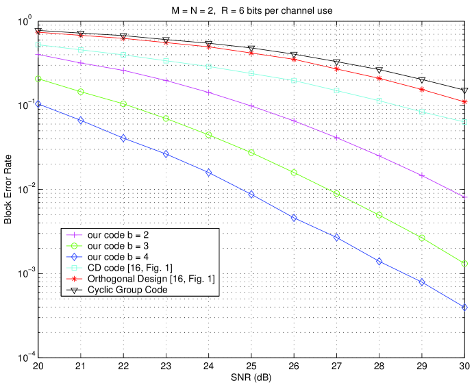
Figure 3: Performance simulations of constellations

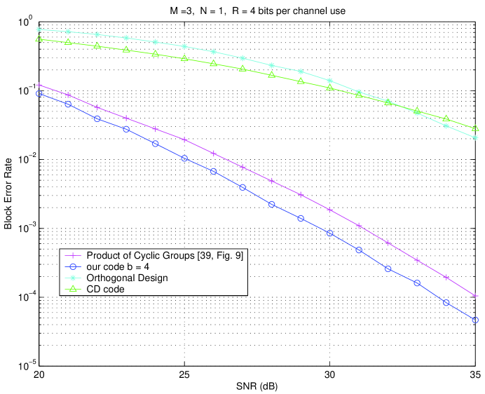
Figure 4: Performance simulations of constellations

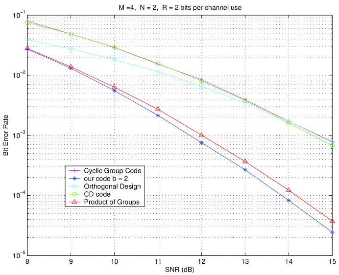
Figure 5: Performance simulations of constellations

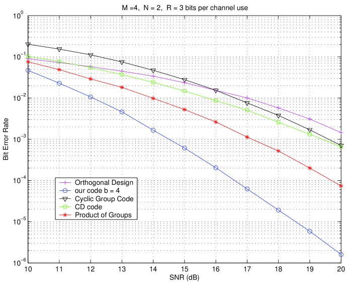
Figure 6: Performance simulations of constellations

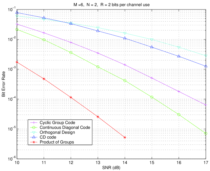
Figure 7: Performance simulations of constellations

5 Conclusion

We have proposed a new class of differential unitary space-time codes which has high performance, low encoding and decoding complexity. We have established a parallel sphere decoder algorithm which efficiently decodes our proposed code and existing codes such as cyclic group code, FPF code $G_{m,r}$, non-group code $S_{m,s}$ and products of groups. We have proposed a new design criterion and powerful optimization techniques for designing unitary space-time codes. We have obtained constellations which significantly improve upon constellations reported in the literature.

Appendix A PROOF OF THEOREM 1

From the illustration after Theorem 2, we see that, the Chernoff bound of the pair-wise error probability is invariant under unitary transforms. By such invariant property, we have

$$P(\Lambda_{p}^{\ell},\Lambda_{p}^{\ell^{{}^{\prime}}})=P(I,\Lambda^{\ell^{{}^{\prime}}-\ell}),\;\;\;\;\;0\leq p\leq 2^{b}-1.$$

Note that

$$d^{\mathrm{H}}(p,p,\ell,\ell^{{}^{\prime}})=d^{\mathrm{H}}(\ell,\ell^{{}^{\prime}})$$

for $0\leq p\leq 2^{b}-1$. Hence

$$\sum_{p=0}^{2^{b}-1}\;\sum_{\ell=0}^{L-2}\;\sum_{\ell^{{}^{\prime}}=\ell+1}^{L-1}d^{\mathrm{H}}(p,p,\ell,\ell^{{}^{\prime}})\;P(\Lambda_{p}^{\ell},\Lambda_{p}^{\ell^{{}^{\prime}}})$$ (22)

$$= 2^{b}\;\sum_{\ell=0}^{L-2}\;\sum_{\ell^{{}^{\prime}}=\ell+1}^{L-1}d^{\mathrm{H}}(\ell,\ell^{{}^{\prime}})\;P(I,\Lambda^{\ell^{{}^{\prime}}-\ell})$$

$$= 2^{b}\;\sum_{k=1}^{L-1}\;\sum_{\ell^{{}^{\prime}}-\ell=k\atop{0\leq\ell\leq L-2\atop{\ell^{{}^{\prime}}\leq L-1}}}d^{\mathrm{H}}(\ell^{{}^{\prime}},\ell)\;P(I,\Lambda^{k}).$$

It can be verified that

$$\sum_{\ell^{{}^{\prime}}-\ell=k\atop{0\leq\ell\leq L-2\atop{\ell^{{}^{\prime}}\leq L-1}}}d^{\mathrm{H}}(\ell^{{}^{\prime}},\ell) = \sum_{0\leq\ell\leq L-k-1}\;d^{\mathrm{H}}(\ell+k,\ell)$$ (23)

$$= w(k).$$

By (22) and (23),

$$\sum_{p=0}^{2^{b}-1}\;\sum_{\ell=0}^{L-2}\;\sum_{\ell^{{}^{\prime}}=\ell+1}^{L-1}d^{\mathrm{H}}(p,p,\ell,\ell^{{}^{\prime}})\;P(\Lambda_{p}^{\ell},\Lambda_{p}^{\ell^{{}^{\prime}}})$$ (24)

$$= 2^{b}\;\sum_{k=1}^{L-1}\;w(k)\;P(I,\Lambda^{k}).$$

Observing that

$$d^{\mathrm{H}}(p,q,\ell,\ell^{{}^{\prime}})=d^{\mathrm{H}}(\ell,\ell^{{}^{\prime}})+d^{\mathrm{H}}(p,q)$$

and

$$P(A_{p}\Lambda_{p}^{\ell}B_{p},\;A_{q}\Lambda_{q}^{\ell^{{}^{\prime}}}B_{q})=P(B_{p},\;\Lambda^{\ell^{{}^{\prime}}-\ell}B_{q}),$$

we have

$$\sum_{\ell=0}^{L-1}\;\sum_{\ell^{{}^{\prime}}=0}^{L-1}d^{\mathrm{H}}(p,q,\ell,\ell^{{}^{\prime}})\;P(A_{p}\Lambda_{p}^{\ell}B_{p},\;A_{q}\Lambda_{q}^{\ell^{{}^{\prime}}}B_{q})$$ (25)

$$= \sum_{\ell=0}^{L-1}\;\sum_{\ell^{{}^{\prime}}=0}^{L-1}d^{\mathrm{H}}(\ell,\ell^{{}^{\prime}})\;P(B_{p},\;\Lambda^{\ell^{{}^{\prime}}-\ell}B_{q})$$

$$+\;\sum_{\ell=0}^{L-1}\;\sum_{\ell^{{}^{\prime}}=0}^{L-1}d^{\mathrm{H}}(p,q)\;P(B_{p},\;\Lambda^{\ell^{{}^{\prime}}-\ell}B_{q})$$

$$= \sum_{k=-L+1}^{L-1}\sum_{\ell^{{}^{\prime}}-\ell=k\atop{0\leq\ell\leq L-1\atop{0\leq\ell^{{}^{\prime}}\leq L-1}}}d^{\mathrm{H}}(\ell,\ell^{{}^{\prime}})\;P(B_{p},\;\Lambda^{k}B_{q})$$

$$+\;d^{\mathrm{H}}(p,q)\;\sum_{k=-L+1}^{L-1}P(B_{p},\;\Lambda^{k}B_{q}).$$

Making use of symmetry, we can show that

$$\sum_{\ell^{{}^{\prime}}-\ell=k\atop{0\leq\ell\leq L-1\atop{0\leq\ell^{{}^{\prime}}\leq L-1}}}d^{\mathrm{H}}(\ell,\ell^{{}^{\prime}})=w(|k|).$$ (26)

By (25) and (26),

$$\sum_{\ell=0}^{L-1}\;\sum_{\ell^{{}^{\prime}}=0}^{L-1}d^{\mathrm{H}}(p,q,\ell,\ell^{{}^{\prime}})\;P(A_{p}\Lambda_{p}^{\ell}B_{p},\;A_{q}\Lambda_{q}^{\ell^{{}^{\prime}}}B_{q})$$ (27)

$$= \sum_{k=-L+1}^{L-1}\;[w(|k|)+d^{\mathrm{H}}(p,q)]\;P(B_{p},\;\Lambda^{k}B_{q}).$$

The proof is finally completed by invoking equations (3),  (24) and  (27).

Appendix B PROOF OF THEOREM 2

By virtue of the Chernoff bound (1),

$$P(U,\Phi)$$

$$= \frac{1}{2}\prod_{m=1}^{M}\left[1+\frac{\rho^{2}\sigma_{m}^{2}}{4(1+2\rho)}\right]^{-N}$$

$$= \frac{\alpha^{MN}}{2}\left[\prod_{m=1}^{M}\left(\alpha+\sigma_{m}^{2}\right)\right]^{-N}$$

where $\sigma_{m}$ is the $m$-th singular value of $U-\Phi$. Let $U_{1}$ and $U_{2}$ be unitary matrices such that $U-\Phi=U_{1}\;{\rm diag}(\sigma_{1},\cdots,\sigma_{M})\;U_{2}^{{\dagger}}$. Then

$$\det[\alpha I+(U-\Phi)(U-\Phi)^{\dagger}]$$ (28)

$$= \det[\alpha I+U_{1}\;{\rm diag}(\sigma_{1}^{2},\cdots,\sigma_{M}^{2})\;U_{1}^{{\dagger}}]$$

$$= \det[U_{1}\;{\rm diag}(\alpha+\sigma_{1}^{2},\cdots,\alpha+\sigma_{M}^{2})\;U_{1}^{{\dagger}}]$$

$$= \det(U_{1}U_{1}^{\dagger})\;\det[{\rm diag}(\alpha+\sigma_{1}^{2},\cdots,\alpha+\sigma_{M}^{2})]$$

$$= \prod_{m=1}^{M}(\alpha+\sigma_{m}^{2}).$$

It follows that

$$P(U,\Phi)=\frac{\alpha^{MN}}{2\left(\det[\alpha I+(U-\Phi)(U-\Phi)^{{\dagger}}]\right)^{N}}$$ (29)

from which we obtain

$$P(I,\Phi) = \frac{\alpha^{MN}}{2\left(\det[\alpha I+(I-\Phi)(I-\Phi)^{{\dagger}}]\right)^{N}}$$

$$= \frac{\alpha^{MN}}{2\left(\det[(\alpha+2)I-\Phi-\Phi^{\dagger}]\right)^{N}}$$

by letting $U=I$. This proves (4).

Now define

$$\Xi \stackrel{{\scriptstyle\mathrm{def}}}{{=}} \log\det[\alpha I+(U-\Phi)(U-\Phi)^{{\dagger}}]$$ (30)

$$= \log\det[(\alpha+2)I-U\Phi^{\dagger}-\Phi U^{\dagger}].$$

By the chain rule of differentiation,

$$\frac{\partial P(U,\Phi)}{\partial\nu_{pq}} = \frac{\partial P(U,\Phi)}{\partial\Xi}\;\frac{\partial\Xi}{\partial\nu_{pq}}$$ (31)

$$= \frac{\partial\left[\frac{\alpha^{MN}}{2}\exp(-N\Xi)\right]}{\partial\Xi}\;\frac{\partial\Xi}{\partial\nu_{pq}}$$

$$= -NP(U,\Phi)\;\frac{\partial\Xi}{\partial\nu_{pq}}.$$

Similarly,

$$\frac{\partial P(U,\Phi)}{\partial\phi_{pq}}=-NP(U,\Phi)\;\frac{\partial\Xi}{\partial\phi_{pq}},$$ (32)

$$\frac{\partial P(U,\Phi)}{\partial\theta_{k}}=-NP(U,\Phi)\;\frac{\partial\Xi}{\partial\theta_{k}}.$$ (33)

Define

$$\Omega\stackrel{{\scriptstyle\mathrm{def}}}{{=}}(\alpha+2)I-U\Phi^{\dagger}-\Phi U^{\dagger}.$$

By (28) and (30),

$$\det(\Omega)=\prod_{m=1}^{M}(\alpha+\sigma_{m}^{2})\geq\alpha^{M}>0$$

for any $U$. Let $e_{j}$ be the $M$-dimensional unit column vector with a one in the $j$-th entry and zeros elsewhere. By the same method of proving (28), we can show that $\det[(\alpha+2)I-(U+e_{j}e_{k}^{\intercal}\delta)\Phi^{\dagger}-\Phi(U^{\dagger}+e_{k}e_{j}^{\intercal}\delta)]$ is a positive real number for any $\delta\in\mathbb{R}$. Since $\det(\Omega)$ is positive and

$$\det[(\alpha+2)I-(U+e_{j}e_{k}^{\intercal}\delta)\Phi^{\dagger}-\Phi(U^{\dagger}+e_{k}e_{j}^{\intercal}\delta)]$$

$$= \det(\Omega)\det[I-\Omega^{-1}(e_{j}e_{k}^{\intercal}\Phi^{\dagger}+\Phi e_{k}e_{j}^{\intercal})\delta],$$

we have that $\det[I-\Omega^{-1}(e_{j}e_{k}^{\intercal}\Phi^{\dagger}+\Phi e_{k}e_{j}^{\intercal})\delta]$ is also a positive real number for any $\delta\in\mathbb{R}$. Therefore,

$$\log\det[(\alpha+2)I-(U+e_{j}e_{k}^{\intercal}\delta)\Phi^{\dagger}-\Phi(U^{\dagger}+e_{k}e_{j}^{\intercal}\delta)]$$

$$= \log\det(\Omega)+\log\det[I-\Omega^{-1}(e_{j}e_{k}^{\intercal}\Phi^{\dagger}+\Phi e_{k}e_{j}^{\intercal})\delta].$$

Let $\Psi=\Omega^{-1}(e_{j}e_{k}^{\intercal}\Phi^{\dagger}+\Phi e_{k}e_{j}^{\intercal})$. Then $\Psi$ is a Hermite matrix, i.e., $\Psi^{\dagger}=\Psi$. It follows that $[\Psi]_{kk}$ is real for $k=1,\cdots,M$. By the definition of a determinant, we have

$$\det(I-\Psi\delta)=\prod_{k=1}^{M}(1-[\Psi]_{kk}\delta)+\delta^{2}f(\delta)>0$$

where $f(.)$ is a polynomial function of $\delta\in\mathbb{R}$. Since $\det(I-\Psi\delta)$ and $[\Psi]_{kk},\;k=1,\cdots,M$ are real numbers, it must be true that $f(\delta)$ is also a real-valued function of $\delta\in\mathbb{R}$. Note that

$$\det(I-\Psi\delta) = 1-\left(\sum_{k=1}^{M}[\Psi]_{kk}\right)\delta+O(\delta^{2})+\delta^{2}f(\delta)$$

$$= 1-{\rm tr}(\Psi)\delta+O(\delta^{2})$$

$$> 0$$

where ${\rm tr}(\Psi)$ is real and $O(\delta^{2})$ is a real-valued function of $\delta\in\mathbb{R}$. Therefore,

$$\log\det(I-\Psi\delta)=-{\rm tr}(\Psi)\delta+O(\delta^{2}).$$ (34)

Making use of (34), we have

$$\log\det[(\alpha+2)I-(U+e_{j}e_{k}^{\intercal}\delta)\Phi^{\dagger}-\Phi(U^{\dagger}+e_{k}e_{j}^{\intercal}\delta)]$$

$$= \log\det(\Omega)-{\rm tr}(\Psi\delta)+O(\delta^{2})$$

$$= \log\det(\Omega)$$

$$-\left[{\rm tr}\left(e_{j}e_{k}^{\intercal}\Phi^{\dagger}\Omega^{-1}\right)+{\rm tr}\left(\Omega^{-1}\Phi e_{k}e_{j}^{\intercal}\right)\right]\delta+O(\delta^{2})$$

$$= \log\det(\Omega)$$

$$-\left[{\rm tr}\left(e_{j}e_{k}^{\intercal}(\Omega^{-1}\Phi)^{\dagger}\right)+{\rm tr}\left(\Omega^{-1}\Phi e_{k}e_{j}^{\intercal}\right)\right]\delta+O(\delta^{2})$$

$$= \log\det(\Omega)$$

$$-\left[{\rm tr}(\left(\Omega^{-1}\Phi e_{k}e_{j}^{\intercal}\right)^{\dagger})+{\rm tr}\left(\Omega^{-1}\Phi e_{k}e_{j}^{\intercal}\right)\right]\delta+O(\delta^{2})$$

$$= \log\det(\Omega)$$

$$-\left[({\rm tr}\left(\Omega^{-1}\Phi e_{k}e_{j}^{\intercal}\right))^{\dagger}+{\rm tr}\left(\Omega^{-1}\Phi e_{k}e_{j}^{\intercal}\right)\right]\delta+O(\delta^{2})$$

$$= \log\det(\Omega)-2\;\Re({\rm tr}\left(\Omega^{-1}\Phi e_{k}e_{j}^{\intercal}\right))\;\delta+O(\delta^{2})$$

$$= \log\det(\Omega)-2\;\Re([\Omega^{-1}\Phi]_{jk})\;\delta+O(\delta^{2})$$

$$= \log\det(\Omega)-2\;[\Re(\Omega^{-1}\Phi)]_{jk}\;\delta+O(\delta^{2})$$

for any $\delta\in\mathbb{R}$. Therefore, applying formula

$$\left[\frac{\partial\;f(X)}{\partial\;\Re(X)}\right]_{jk}=\lim_{\delta\rightarrow 0}\frac{f(X+e_{j}e_{k}^{\intercal}\delta)-f(X)}{\delta}$$

provided in [16] (page 1501), we have

$$\left[\frac{\partial\;\Xi}{\partial\;\Re(U)}\right]_{jk}$$

$$= \lim_{\delta\rightarrow 0}\frac{\log\det[\Omega-(e_{j}e_{k}^{\intercal}\Phi^{\dagger}+\Phi e_{k}e_{j}^{\intercal})\delta]-\log\det(\Omega)}{\delta}$$

$$= \lim_{\delta\rightarrow 0}\frac{-2[\Re(\Omega^{-1}\Phi)]_{jk}\;\delta+O(\delta^{2})}{\delta}$$

$$= -2[\Re(\Omega^{-1}\Phi)]_{jk}.$$

Observing that $U=I$ for $\Theta=0$ (i.e., all elements of $\Theta$ are zeros), we have $\Omega=(\alpha+2)I-\Phi-\Phi^{\dagger}$ and $\Omega^{-1}\Phi=[(\alpha+2)I-\Phi-\Phi^{{\dagger}}]^{-1}\Phi=\mathcal{Q}$. Hence,

$$\left.\frac{\partial\;\Xi}{\partial\;\Re(U)}\right|_{\Theta=0}=-2\Re(\mathcal{Q}).$$ (35)

Similarly,

$$\log\det[(\alpha+2)I-(U+e_{j}e_{k}^{\intercal}\delta i)\Phi^{\dagger}-\Phi(U^{\dagger}-e_{k}e_{j}^{\intercal}\delta i)]$$

$$= \log\det[\Omega-(e_{j}e_{k}^{\intercal}\Phi^{\dagger}-\Phi e_{k}e_{j}^{\intercal})\delta i]$$

$$= \log\det(\Omega)+\log\det[I-\Omega^{-1}(e_{j}e_{k}^{\intercal}\Phi^{\dagger}-\Phi e_{k}e_{j}^{\intercal})\delta i]$$

$$= \log\det(\Omega)-{\rm tr}[\Omega^{-1}(e_{j}e_{k}^{\intercal}\Phi^{\dagger}-\Phi e_{k}e_{j}^{\intercal})\delta i]+O(\delta^{2})$$

$$= \log\det(\Omega)$$

$$-\left[{\rm tr}\left(e_{j}e_{k}^{\intercal}\Phi^{\dagger}\Omega^{-1}\right)-{\rm tr}\left(\Omega^{-1}\Phi e_{k}e_{j}^{\intercal}\right)\right]\delta i+O(\delta^{2})$$

$$= \log\det(\Omega)$$

$$-\left[{\rm tr}\left(e_{j}e_{k}^{\intercal}(\Omega^{-1}\Phi)^{\dagger}\right)-{\rm tr}\left(\Omega^{-1}\Phi e_{k}e_{j}^{\intercal}\right)\right]\delta i+O(\delta^{2})$$

$$= \log\det(\Omega)$$

$$-\left[{\rm tr}(\left(\Omega^{-1}\Phi e_{k}e_{j}^{\intercal}\right)^{\dagger})-{\rm tr}\left(\Omega^{-1}\Phi e_{k}e_{j}^{\intercal}\right)\right]\delta i+O(\delta^{2})$$

$$= \log\det(\Omega)$$

$$-\left[({\rm tr}\left(\Omega^{-1}\Phi e_{k}e_{j}^{\intercal}\right))^{\dagger}-{\rm tr}\left(\Omega^{-1}\Phi e_{k}e_{j}^{\intercal}\right)\right]\delta i+O(\delta^{2})$$

$$= \log\det(\Omega)-2\;\Im({\rm tr}\left(\Omega^{-1}\Phi e_{k}e_{j}^{\intercal}\right))\;\delta+O(\delta^{2})$$

$$= \log\det(\Omega)-2\;\Im([\Omega^{-1}\Phi]_{jk})\;\delta+O(\delta^{2})$$

$$= \log\det(\Omega)-2\;[\Im(\Omega^{-1}\Phi)]_{jk}\;\delta+O(\delta^{2})$$

for any $\delta\in\mathbb{R}$. Therefore,

$$\left[\frac{\partial\;\Xi}{\partial\;\Im(U)}\right]_{jk}$$

$$= \lim_{\delta\rightarrow 0}\frac{\log\det[\Omega-(e_{j}e_{k}^{\intercal}\Phi^{\dagger}-\Phi e_{k}e_{j}^{\intercal})\delta i]-\log\det(\Omega)}{\delta}$$

$$= \lim_{\delta\rightarrow 0}\frac{-2[\Im(\Omega^{-1}\Phi)]_{jk}\;\delta+O(\delta^{2})}{\delta}$$

$$= -2[\Im(\mathcal{Q})]_{jk}$$

for $\Theta=0$, which implies that

$$\left.\frac{\partial\;\Xi}{\partial\;\Im(U)}\right|_{\Theta=0}=-2\Im(\mathcal{Q}).$$ (36)

We now consider the partial derivatives of $U$ with respective to the elements of $\Theta$. It should be noted that an incorrect formula for computing ${\left.\frac{\partial U}{\partial\phi_{pq}}\right|}_{\Theta=0}$ has been reported in [1] (see equation (13), page 2625). In the sequel, we shall prove that

$${\left.\frac{\partial U}{\partial\phi_{pq}}\right|}_{\Theta=0}=e_{q}e_{p}^{\intercal}-e_{p}e_{q}^{\intercal},$$ (37)

which is clearly different from equation (13) of [1]. To that end, we can use the parameterization of unitary matrix $U(\Theta)$ to verify that

$${\left.\frac{\partial U}{\partial\phi_{pq}}\right|}_{\Theta=0}={\left.\frac{\partial\widetilde{U}}{\partial\phi_{pq}}\right|}_{\phi_{pq}=0}$$

where

$$\widetilde{U}=\left[\begin{array}[]{ll}I_{(p-1)\times(p-1)}&0_{(p-1)\times(M-p+1)}\\ 0_{(M-p+1)\times(p-1)}&U^{p,q}(\phi_{pq},0)\end{array}\right]$$

with

$$[U^{p,q}(\phi_{pq},0)]_{jk}$$

$$= \left\{\begin{array}[]{ll}1,&{\rm if}\;j=k\;{\rm and}\;j\notin\{1,\;q-p+1\}\\ \cos(\phi_{pq}),&{\rm if}\;j=k\;{\rm and}\;j\in\{1,\;q-p+1\}\\ -\sin(\phi_{pq}),&{\rm if}\;j=1\;{\rm and}\;k=q-p+1\\ \sin(\phi_{pq}),&{\rm if}\;k=1\;{\rm and}\;j=q-p+1\\ 0,&{\rm otherwise.}\end{array}\right.$$

Obviously,

$$\left.\frac{\partial\;([U^{p,q}(\phi_{pq},0)]_{jk})}{\partial\phi_{pq}}\right|_{\phi_{pq}=0}$$

$$= \left\{\begin{array}[]{ll}-1,&{\rm if}\;j=1\;{\rm and}\;k=q-p+1\\ 1,&{\rm if}\;k=1\;{\rm and}\;j=q-p+1\\ 0,&{\rm otherwise.}\end{array}\right.$$

Hence, (37) can be obtained by observing that

$$[\widetilde{U}]_{pq}=[U^{p,q}(\phi_{pq},0)]_{1,q-p+1},$$

$$[\widetilde{U}]_{qp}=[U^{p,q}(\phi_{pq},0)]_{q-p+1,1}.$$

To compute other partial derivatives of $U(\Theta)$ at $\Theta=0$, we quote equations (14) and (15) of [1] as follows:

$${\left.\frac{\partial U}{\partial\nu_{pq}}\right|}_{\Theta=0}=0,\;\;\;\;\;{\left.\frac{\partial U}{\partial\theta_{k}}\right|}_{\Theta=0}=ie_{k}e_{k}^{\intercal}.$$ (40)

By virtue of (37) and (40),

$${\left.\frac{\partial\;\Re(U)}{\partial\phi_{pq}}\right|}_{\Theta=0}=e_{q}e_{p}^{\intercal}-e_{p}e_{q}^{\intercal},\;\;\;\;\;\;{\left.\frac{\partial\;\Im(U)}{\partial\phi_{pq}}\right|}_{\Theta=0}=0,$$ (41)

$${\left.\frac{\partial\;\Re(U)}{\partial\nu_{pq}}\right|}_{\Theta=0}=0,\;\;\;\;\;\;\;\;\;\;\;\;\;\;\;\;\;\;\;\;\;{\left.\frac{\partial\;\Im(U)}{\partial\nu_{pq}}\right|}_{\Theta=0}=0,$$ (42)

$${\left.\frac{\partial\;\Re(U)}{\partial\theta_{k}}\right|}_{\Theta=0}=0,\;\;\;\;\;\;\;\;\;\;\;\;\;\;\;\;\;{\left.\frac{\partial\;\Im(U)}{\partial\theta_{k}}\right|}_{\Theta=0}=e_{k}e_{k}^{\intercal}.$$ (43)

We now define inner product $<.,.>$ by

$$<X,Y>\stackrel{{\scriptstyle\mathrm{def}}}{{=}}\sum_{j,k}[X]_{jk}\;[Y]_{jk}.$$

Then by the chain rule of differentiation and equations (35), (41), we have

$$\frac{\partial\;\Xi}{\partial\phi_{pq}} = \left<\frac{\partial\;\Xi}{\partial\;\Re(U)},\frac{\partial\;\Re(U)}{\partial\phi_{pq}}\right>+\left<\frac{\partial\;\Xi}{\partial\;\Im(U)},\frac{\partial\;\Im(U)}{\partial\phi_{pq}}\right>$$

$$= \left<\frac{\partial\;\Xi}{\partial\;\Re(U)},\frac{\partial\;\Re(U)}{\partial\phi_{pq}}\right>$$

$$= \left<-2\;\Re(\mathcal{Q}),\;e_{q}e_{p}^{\intercal}-e_{p}e_{q}^{\intercal}\right>$$

$$= -2\;\Re\left(\left<\mathcal{Q},\;e_{q}e_{p}^{\intercal}-e_{p}e_{q}^{\intercal}\right>\right)$$

$$= -2\;\Re([\mathcal{Q}]_{qp}-[\mathcal{Q}]_{pq}).$$

Invoking (32) yields

$$\frac{\partial\;P(U,\Phi)}{\partial\phi_{pq}} = -NP(U,\Phi)\frac{\partial\;\Xi}{\partial\phi_{pq}}$$

$$= 2NP(U,\Phi)\;\Re([\mathcal{Q}]_{qp}-[\mathcal{Q}]_{pq})$$

and hence proves (5).

By the chain rule of differentiation and (42),

$$\frac{\partial\;\Xi}{\partial\nu_{pq}}=\left<\frac{\partial\;\Xi}{\partial\;\Re(U)},\frac{\partial\;\Re(U)}{\partial\nu_{pq}}\right>+\left<\frac{\partial\;\Xi}{\partial\;\Im(U)},\frac{\partial\;\Im(U)}{\partial\nu_{pq}}\right>=0.$$ (44)

Combing (31) and (44) leads to

$$\frac{\partial\;P(U,\Phi)}{\partial\nu_{pq}}=0$$

and thus completes the proof of (7).

By the chain rule of differentiation and (43),

$$\frac{\partial\;\Xi}{\partial\theta_{k}} = \left<\frac{\partial\;\Xi}{\partial\;\Re(U)},\frac{\partial\;\Re(U)}{\partial\theta_{k}}\right>+\left<\frac{\partial\;\Xi}{\partial\;\Im(U)},\frac{\partial\;\Im(U)}{\partial\theta_{k}}\right>$$

$$= \left<\frac{\partial\;\Xi}{\partial\;\Im(U)},\frac{\partial\;\Im(U)}{\partial\theta_{k}}\right>$$

$$= \left<-2\;\Im(\mathcal{Q}),\;\;e_{k}e_{k}^{\intercal}\right>$$

$$= -2\;\Im\left(\left<\mathcal{Q},\;\;e_{k}e_{k}^{\intercal}\right>\right)$$

$$= -2\;\Im([\mathcal{Q}]_{kk}).$$

Hence by (33), we have

$$\frac{\partial\;P(U,\Phi)}{\partial\theta_{k}} = -NP(U,\Phi)\;\frac{\partial\;\Xi}{\partial\theta_{k}}$$

$$= 2NP(U,\Phi)\;\Im([\mathcal{Q}]_{kk})$$

and completes the proof of (6).

Define

$$\Upsilon\stackrel{{\scriptstyle\mathrm{def}}}{{=}}\log\det[\alpha I+(\Lambda^{\ell}-\Phi)(\Lambda^{\ell}-\Phi)^{{\dagger}}].$$

By the same method as computing $\frac{\partial\;\Xi}{\partial\;\Im(U)}$, we have

$$\frac{\partial\;\Upsilon}{\partial\;\Im(\Lambda^{\ell})}=-2\Im(\mathcal{Q}).$$ (45)

Observing that $[\Lambda^{\ell}]_{jk}$ depends on $\lambda_{m}$ only if $j=k=m$ and that

$${\left.\frac{\partial\;\Re([\Lambda^{\ell}]_{mm})}{\partial\lambda_{m}}\right|}_{\Lambda=I}={\left.\frac{\partial\;\cos(\frac{2\pi\ell\lambda_{m}}{L})}{\partial\lambda_{m}}\right|}_{\Lambda=I}=0$$

$${\left.\frac{\partial\;\Im([\Lambda^{\ell}]_{mm})}{\partial\lambda_{m}}\right|}_{\Lambda=I}={\left.\frac{\partial\;\sin(\frac{2\pi\ell\lambda_{m}}{L})}{\partial\lambda_{m}}\right|}_{\Lambda=I}=\frac{2\pi\ell}{L},$$

we have

$${\left.\frac{\partial\;\Re(\Lambda^{\ell})}{\partial\lambda_{m}}\right|}_{\Lambda=I}=0,\;\;\;{\left.\frac{\partial\;\Im(\Lambda^{\ell})}{\partial\lambda_{m}}\right|}_{\Lambda=I}=\frac{2\pi\ell}{L}e_{m}e_{m}^{\intercal}.$$ (46)

By the chain rule of differentiation and equations (45), (46), we have

$$\frac{\partial\;\Upsilon}{\partial\lambda_{m}} = \left<\frac{\partial\;\Upsilon}{\partial\;\Re(\Lambda^{\ell})},\frac{\partial\;\Re(\Lambda^{\ell})}{\partial\lambda_{m}}\right>+\left<\frac{\partial\;\Upsilon}{\partial\;\Im(\Lambda^{\ell})},\frac{\partial\;\Im(\Lambda^{\ell})}{\partial\lambda_{m}}\right>$$

$$= \left<\frac{\partial\;\Upsilon}{\partial\;\Im(\Lambda^{\ell})},\frac{\partial\;\Im(\Lambda^{\ell})}{\partial\lambda_{m}}\right>$$

$$= \left<-2\Im(\mathcal{Q}),\frac{2\pi\ell}{L}e_{m}e_{m}^{\intercal}\right>$$

$$= -\frac{4\pi\ell}{L}\Im([\mathcal{Q}]_{mm}).$$

It follows that

$$\frac{\partial\;P(\Lambda^{\ell},\Phi)}{\partial\lambda_{m}} = -NP(\Lambda^{\ell},\Phi)\;\frac{\partial\;\Upsilon}{\partial\lambda_{m}}$$

$$= \frac{4\pi\ell NP(\Lambda^{\ell},\Phi)}{L}\;\Im([\mathcal{Q}]_{mm})$$

and (8) is true.

Appendix C PROOF OF THEOREM 3

First we need to prove some preliminary results.

Lemma 1

For any $\ell\in\{0,1,\cdots,L-1\}$, there exists $y\in\mathcal{S}$ such that

$$\sum_{m=1}^{M}[(C_{m}\lambda_{m}\;\ell-C_{m}\varphi_{m})\;{\rm mod}^{*}C_{m}L]^{2}=||y\;G-\xi||^{2}.$$ (47)

Proof.

Given $\ell\in\{0,1,\cdots,L-1\}$, define

$$y_{1}=\ell+\left\lceil\frac{\varphi_{1}-\ell}{L}-\frac{1}{2}\right\rceil L.$$ (48)

We claim that

$$-\frac{L}{2}+\varphi_{1}\leq y_{1}<\frac{L}{2}+\varphi_{1}.$$ (49)

To prove (49), one can make use of the observation that

$$0\leq\lceil x\rceil-x<1\;\;\forall x\in\mathbb{R}$$

and verify that inequality

$$0\leq\left\lceil\frac{\varphi_{1}-\ell}{L}-\frac{1}{2}\right\rceil-\left(\frac{\varphi_{1}-\ell}{L}-\frac{1}{2}\right)<1$$

is equivalent to

$$-\frac{L}{2}+\varphi_{1}\leq\ell+\left\lceil\frac{\varphi_{1}-\ell}{L}-\frac{1}{2}\right\rceil L<\frac{L}{2}+\varphi_{1}.$$

The truth of (49) allows one to choose $y=[y_{1},\;\cdots,y_{M}]\in\mathcal{S}$ such that the first entry of $y$ is $y_{1}$. Let

$$w=[w_{1},\cdots,w_{M}]=y\;G-\xi.$$ (50)

Obviously, to show (47), it suffices to show

$$(C_{m}\lambda_{m}\;\ell-C_{m}\varphi_{m})\;{\rm mod}^{*}C_{m}L=w_{m},\;\;\;m=1,\cdots,M$$

where $\lambda_{1}=1$. By the definitions of $G$ and $\xi$, we can rewrite (50) as

$$w_{1}=C_{1}y_{1}-C_{1}\varphi_{1},$$

$$w_{m}=C_{m}\lambda_{m}\;y_{1}+C_{m}L\;y_{m}-C_{m}\varphi_{m}\;\;{\rm for}\;\;m=2,\cdots,M.$$

Hence, to show (47), it suffices to show

$$(C_{1}\;\ell-C_{1}\varphi_{1})\;{\rm mod}^{*}C_{1}L=C_{1}y_{1}-C_{1}\varphi_{1}$$ (51)

and, for $m=2,\cdots,M$,

$$(C_{m}\lambda_{m}\;\ell-C_{m}\varphi_{m})\;{\rm mod}^{*}C_{m}L$$ (52)

$$= C_{m}\lambda_{m}\;y_{1}+C_{m}L\;y_{m}-C_{m}\varphi_{m}.$$

Note that, for any $\ell$, there exits an unique integer $z_{1}$ such that

$$(C_{1}\;\ell-C_{1}\varphi_{1})\;{\rm mod}^{*}C_{1}L=C_{1}\;\ell-C_{1}\varphi_{1}+z_{1}C_{1}L.$$

Therefore, to show (51), it suffices to show

$$C_{1}y_{1}-C_{1}\varphi_{1}=C_{1}\;\ell-C_{1}\varphi_{1}+z_{1}C_{1}L,$$

or equivalently,

$$z_{1}=\frac{y_{1}-\ell}{L}.$$ (53)

By the definition of the symmetric modulus operator ${\rm mod}^{*}$, integer $z_{1}$ guarantees

$$-\frac{C_{1}L}{2}\leq C_{1}\;\ell-C_{1}\varphi_{1}+z_{1}C_{1}L<\frac{C_{1}L}{2},$$

or equivalently,

$$-1<\left(\frac{\varphi_{1}-\ell}{L}-\frac{1}{2}\right)-z_{1}\leq 0,$$

which implies

$$\left\lceil\frac{\varphi_{1}-\ell}{L}-\frac{1}{2}-z_{1}\right\rceil=0.$$

Since $z_{1}$ is an integer, we have

$$z_{1} = \left\lceil\frac{\varphi_{1}-\ell}{L}-\frac{1}{2}\right\rceil$$

$$= \frac{y_{1}-\ell}{L}$$

where the second equality follows from (48). So equation (51) is proven by invoking (53).

In light of the fact that, for any given $\ell\in\{0,1,\cdots,L-1\}$ and for any $m\in\{2,\cdots,M\}$, there exists an unique integer $z_{m}$ such that

$$(C_{m}\lambda_{m}\;\ell-C_{m}\varphi_{m})\;{\rm mod}^{*}C_{m}L=C_{m}(\lambda_{m}\ell-\varphi_{m}+z_{m}L),$$

to show (52) it suffices to prove that

$$C_{m}(\lambda_{m}\ell-\varphi_{m}+z_{m}L)=C_{m}\lambda_{m}\;y_{1}+C_{m}L\;y_{m}-C_{m}\varphi_{m}$$

for $m=2,\cdots,M$, or equivalently,

$$y_{m}=z_{m}-\frac{y_{1}-\ell}{L}\lambda_{m},\;\;\;\;\;\;m=2,\cdots,M.$$ (54)

By the definition of the symmetric modulus operator ${\rm mod}^{*}$, integer $z_{m}$ guarantees

$$-\frac{C_{m}L}{2}\leq C_{m}\lambda_{m}\;\ell-C_{m}\varphi_{m}+z_{m}C_{m}L<\frac{C_{m}L}{2}$$

which can be rewritten as

$$-\frac{C_{m}L}{2}\leq C_{m}[\lambda_{m}(\ell+z_{1}L)-\varphi_{m}+(z_{m}-z_{1}\lambda_{m})L]<\frac{C_{m}L}{2},$$

i.e.,

$$-1<\left(\frac{\varphi_{m}}{L}-\left(\frac{\ell+z_{1}L}{L}-z_{1}\right)\;\lambda_{m}-\frac{1}{2}\right)-z_{m}\leq 0$$

for $m=2,\cdots,M$. Therefore,

$$\left\lceil\left(\frac{\varphi_{m}}{L}-\left(\frac{\ell+z_{1}L}{L}-z_{1}\right)\;\lambda_{m}-\frac{1}{2}\right)-z_{m}\right\rceil=0$$

for $m=2,\cdots,M$. Since $z_{m}$ is an integer, we have

$$z_{m} = \left\lceil\frac{\varphi_{m}}{L}-\left(\frac{\ell+z_{1}L}{L}-z_{1}\right)\;\lambda_{m}-\frac{1}{2}\right\rceil$$ (55)

$$= \left\lceil\frac{\varphi_{m}}{L}-\left(\frac{y_{1}}{L}-z_{1}\right)\;\lambda_{m}-\frac{1}{2}\right\rceil$$

for $m=2,\cdots,M$. Here (55) is due to (53). By the definition of $\mathcal{S}$,

$$y_{m}=\left\lceil\frac{\varphi_{m}}{L}-\left(\frac{y_{1}}{L}-\left\lfloor\frac{y_{1}}{L}\right\rfloor\right)\;\lambda_{m}-\frac{1}{2}\right\rceil-\left\lfloor\frac{y_{1}}{L}\right\rfloor\;\lambda_{m}.$$ (56)

By virtue of (53) and the fact that $0\leq\ell<L$, we have

$$0\leq\frac{y_{1}}{L}-z_{1}<1,$$

which leads to

$$\left\lfloor\frac{y_{1}}{L}-z_{1}\right\rfloor=0$$

and consequently

$$z_{1}=\left\lfloor\frac{y_{1}}{L}\right\rfloor.$$ (57)

Combining (53), (55), (56) and (57) yields

$$y_{m} = \left\lceil\frac{\varphi_{m}}{L}-\left(\frac{y_{1}}{L}-z_{1}\right)\;\lambda_{m}-\frac{1}{2}\right\rceil-z_{1}\;\lambda_{m}$$

$$= z_{m}-z_{1}\lambda_{m}$$

$$= z_{m}-\frac{y_{1}-\ell}{L}\lambda_{m}$$

for $m=2,\cdots,M$. This proves (54). It follows that (52) is true and the lemma is thus proven.

$\Box$

Lemma 2

Let $y=[y_{1},\;\cdots,y_{M}]\in\mathcal{S}$. If $\widetilde{\ell}=y_{1}-\left\lfloor\frac{y_{1}}{L}\right\rfloor L$, then $0\leq\widetilde{\ell}<L$ and

$$\sum_{m=1}^{M}[(C_{m}\lambda_{m}\;\widetilde{\ell}-C_{m}\varphi_{m})\;{\rm mod}^{*}C_{m}L]^{2}=||y\;G-\xi||^{2}.$$ (58)

Proof.

By the definition of $\widetilde{\ell}$,

$$\frac{\widetilde{\ell}}{L}=\frac{y_{1}}{L}-\left\lfloor\frac{y_{1}}{L}\right\rfloor\in[0,1).$$

Hence, $0\leq\widetilde{\ell}<L$. Clearly, there uniquely exist integers $\widetilde{z}_{1},\cdots,\widetilde{z}_{M}$ such that, for $m=1,\cdots,M$,

$$(C_{m}\lambda_{m}\;\widetilde{\ell}-C_{m}\varphi_{m})\;{\rm mod}^{*}C_{m}L=C_{m}\lambda_{m}\;\widetilde{\ell}+\widetilde{z}_{m}C_{m}L-C_{m}\varphi_{m}$$

where $\lambda_{1}=1$. Therefore, to prove (58) it suffices to show

$$C_{1}\;\widetilde{\ell}+\widetilde{z}_{1}C_{1}L-C_{1}\varphi_{1}=C_{1}y_{1}-C_{1}\varphi_{1}$$ (59)

and, for $m=2,\cdots,M$,

$$C_{m}\lambda_{m}\;\widetilde{\ell}+\widetilde{z}_{m}C_{m}L-C_{m}\varphi_{m}=C_{m}\lambda_{m}\;y_{1}+C_{m}L\;y_{m}-C_{m}\varphi_{m}.$$ (60)

Equation (59) can be simplified as

$$\widetilde{\ell}+\widetilde{z}_{1}L=y_{1},$$ (61)

which can be further reduced to

$$\widetilde{z}_{1}=\left\lfloor\frac{y_{1}}{L}\right\rfloor$$ (62)

by invoking the definition of $\widetilde{\ell}$. By the definition of the symmetric modulus operator ${\rm mod}^{*}$,

$$-\frac{C_{1}L}{2}\leq C_{1}\;\widetilde{\ell}+\widetilde{z}_{1}C_{1}L-C_{1}\varphi_{1}<\frac{C_{1}L}{2},$$

which can be rewritten as

$$-1<\left(\frac{\varphi_{1}-\widetilde{\ell}}{L}-\frac{1}{2}\right)-\widetilde{z}_{1}\leq 0,$$

or equivalently,

$$\left\lceil\left(\frac{\varphi_{1}-\widetilde{\ell}}{L}-\frac{1}{2}\right)-\widetilde{z}_{1}\right\rceil=0.$$ (63)

By virtue of (63) and the definition of $\widetilde{\ell}$,

$$\widetilde{z}_{1} = \left\lceil\frac{\varphi_{1}-\widetilde{\ell}}{L}-\frac{1}{2}\right\rceil$$ (64)

$$= \left\lceil\frac{\varphi_{1}-(y_{1}-\left\lfloor\frac{y_{1}}{L}\right\rfloor L)}{L}-\frac{1}{2}\right\rceil$$

$$= \left\lceil\frac{\varphi_{1}}{L}-\frac{y_{1}}{L}-\frac{1}{2}\right\rceil+\left\lfloor\frac{y_{1}}{L}\right\rfloor.$$

Remember that $y_{1}$ is restricted by condition

$$-\frac{L}{2}+\varphi_{1}\leq y_{1}<\frac{L}{2}+\varphi_{1},$$

or equivalently

$$-1<\frac{\varphi_{1}}{L}-\frac{y_{1}}{L}-\frac{1}{2}\leq 0$$

which implies

$$\left\lceil\frac{\varphi_{1}}{L}-\frac{y_{1}}{L}-\frac{1}{2}\right\rceil=0.$$ (65)

Combining (64) with (65) yields (62) and consequently proves (59).

We now turn our attention to the proof of (60). By the definition of $\widetilde{\ell}$, (60) can be rewritten as

$$\lambda_{m}\left(y_{1}-\left\lfloor\frac{y_{1}}{L}\right\rfloor L\right)+\widetilde{z}_{m}L=y_{1}\lambda_{m}+y_{m}L,$$

which can be further simplified as

$$\widetilde{z}_{m}=y_{m}+\left\lfloor\frac{y_{1}}{L}\right\rfloor\lambda_{m}.$$ (66)

By the definition of the symmetric modulus operator ${\rm mod}^{*}$, we have

$$-\frac{C_{m}L}{2}\leq C_{m}\lambda_{m}\;\widetilde{\ell}+\widetilde{z}_{m}C_{m}L-C_{m}\varphi_{m}<\frac{C_{m}L}{2},$$

which can be rewritten as

$$-\frac{C_{m}L}{2}\leq C_{m}[\lambda_{m}(\widetilde{\ell}+\widetilde{z}_{1}L)+(\widetilde{z}_{m}-\widetilde{z}_{1}\lambda_{m})L-\varphi_{m}]<\frac{C_{m}L}{2},$$

or equivalently,

$$-1<\frac{\varphi_{m}}{L}-\left(\frac{\widetilde{\ell}+\widetilde{z}_{1}L}{L}-\widetilde{z}_{1}\right)\lambda_{m}-\frac{1}{2}-\widetilde{z}_{m}\leq 0.$$

Hence,

$$\left\lceil\frac{\varphi_{m}}{L}-\left(\frac{\widetilde{\ell}+\widetilde{z}_{1}L}{L}-\widetilde{z}_{1}\right)\lambda_{m}-\frac{1}{2}-\widetilde{z}_{m}\right\rceil=0.$$

Since $\widetilde{z}_{m}$ is an integer, it can be determined that

$$\widetilde{z}_{m}=\left\lceil\frac{\varphi_{m}}{L}-\left(\frac{\widetilde{\ell}+\widetilde{z}_{1}L}{L}-\widetilde{z}_{1}\right)\lambda_{m}-\frac{1}{2}\right\rceil.$$ (67)

Note that (61) is true since (62) has been established. Using (61), (62) and (67), we obtain

$$\widetilde{z}_{m}=\left\lceil\frac{\varphi_{m}}{L}-\left(\frac{y_{1}}{L}-\left\lfloor\frac{y_{1}}{L}\right\rfloor\right)\lambda_{m}-\frac{1}{2}\right\rceil.$$ (68)

Invoking (56) and (68) leads to (66). This proves (60) and the proof of the lemma is thus completed.

$\Box$

We are now in position to prove Theorem 3. By Lemma 1, we have

$$\min_{\ell}\;\sum_{m=1}^{M}[(C_{m}\lambda_{m}\;\ell-C_{m}\varphi_{m})\;{\rm mod}^{*}C_{m}L]^{2}\;\geq\;\min_{y\in\mathcal{S}}\;||yG-\xi||^{2}.$$

On the other hand, by Lemma 2, we have

$$\min_{\ell}\;\sum_{m=1}^{M}[(C_{m}\lambda_{m}\;\ell-C_{m}\varphi_{m})\;{\rm mod}^{*}C_{m}L]^{2}\;\leq\;\min_{y\in\mathcal{S}}\;||yG-\xi||^{2}.$$

Therefore,

$$\min_{\ell}\;\sum_{m=1}^{M}[(C_{m}\lambda_{m}\;\ell-C_{m}\varphi_{m})\;{\rm mod}^{*}C_{m}L]^{2}\;=\;\min_{y\in\mathcal{S}}\;||yG-\xi||^{2}.$$

Since $\widehat{y}_{1}$ is the first entry of

$$\widehat{y}=[\widehat{y}_{1},\cdots,\widehat{y}_{M}]\;=\;\arg\;\min_{y\in\mathcal{S}}\;||yG-\xi||^{2}$$

and $\widehat{\ell}$ is unique, it follows from Lemma 2 that

$$\widehat{\ell} = \arg\;\min_{\ell}\;\sum_{m=1}^{M}[(C_{m}\lambda_{m}\;\ell-C_{m}\varphi_{m})\;{\rm mod}^{*}C_{m}L]^{2}$$

$$= \;\widehat{y}_{1}-\left\lfloor\frac{\widehat{y}_{1}}{L}\right\rfloor\;L.$$

The proof of Theorem 3 is thus completed.

Appendix D PROOF OF THEOREM 4

By the definitions of $G$ and $\xi$,

$$||yG-\xi||^{2}=[C_{1}(y_{1}-\varphi_{1})]^{2}+\sum_{m=2}^{M}[C_{m}(\lambda_{m}\;y_{1}+L\;y_{m}-\varphi_{m})]^{2}.$$

Note that

$$[C_{1}(y_{1}-\varphi_{1})]^{2}+\sum_{m=2}^{M}[C_{m}(\lambda_{m}\;y_{1}+L\;y_{m}-\varphi_{m})]^{2}<\gamma^{2}$$

if and only if

$$[C_{1}(y_{1}-\varphi_{1})]^{2}<\gamma^{2},$$ (69)

$$[C_{1}(y_{1}-\varphi_{1})]^{2}+\sum_{p=2}^{m}[C_{p}(\lambda_{p}\;y_{1}+L\;y_{p}-\varphi_{p})]^{2}<\gamma^{2}$$

$$\;\;\;\;{\rm for}\;\;\;\;m=2,\cdots,M.$$ (70)

Inequalities (69) and (70) can be shown to be equivalent to (14) and (15) by invoking the definitions of $\mathcal{S}$ and $\mu_{m}$.

Appendix E DATA OF UNITARY SPACE-TIME CODES

Constellation for $M=N=b=2,\;L=1024,\;R=6$

For $q=0,1,2,3$,

$$\Lambda_{q}={\rm diag}\left(\exp\left(\frac{2\pi i}{L}[1\;\;376]\right)\right),$$

$$A_{q}=B_{0}=I_{2\times 2}.$$

$$B_{1}=\left[\begin{array}[]{rr}0.5192+0.1730i&0.7689+0.3305i\\ 0.3249+0.7713i&-0.1692-0.5205i\end{array}\right],$$

$$B_{2}=\left[\begin{array}[]{rr}0.4772-0.3219i&0.0907+0.8127i\\ -0.1774+0.7983i&0.4398+0.3713i\end{array}\right],$$

$$B_{3}=\left[\begin{array}[]{rr}-0.4458+0.3772i&0.7645+0.2729i\\ -0.6303+0.5115i&-0.5459-0.2075i\end{array}\right].$$

See Figure 3 for the corresponding performance simulation results.

Constellation for $M=N=2,\;b=3,\;L=512,\;R=6$

For $q=0,1,\cdots,7$,

$$\Lambda_{q}={\rm diag}\left(\exp\left(\frac{2\pi i}{L}[1\;\;188]\right)\right),$$

$$A_{q}=B_{0}=I_{2\times 2}.$$

$$B_{1}=\left[\begin{array}[]{rr}0.3408+0.6630i&-0.1400-0.6517i\\ -0.2401+0.6218i&-0.4402+0.6016i\end{array}\right],$$

$$B_{2}=\left[\begin{array}[]{rr}0.4230+0.2881i&-0.7279+0.4563i\\ 0.8585+0.0319i&0.2226-0.4609i\end{array}\right],$$

$$B_{3}=\left[\begin{array}[]{rr}0.3663+0.1357i&0.8257+0.4069i\\ -0.5379-0.7470i&0.1944+0.3388i\end{array}\right],$$

$$B_{4}=\left[\begin{array}[]{rr}0.7428+0.1845i&0.4221-0.4858i\\ -0.6130-0.1962i&0.5391-0.5433i\end{array}\right],$$

$$B_{5}=\left[\begin{array}[]{rr}0.2656-0.1927i&-0.9238+0.1975i\\ 0.3009+0.8954i&-0.0304+0.3267i\end{array}\right],$$

$$B_{6}=\left[\begin{array}[]{rr}0.0816+0.8219i&-0.4396-0.3530i\\ 0.3081+0.4722i&0.8099+0.1620i\end{array}\right],$$

$$B_{7}=\left[\begin{array}[]{rr}-0.0442-0.7407i&0.5677-0.3564i\\ -0.5320-0.4079i&-0.1131+0.7334i\end{array}\right].$$

See Figure 3 for the corresponding performance simulation results.

Constellation for $M=N=2,\;b=4,\;L=256,\;R=6$

For $q=0,1,\cdots,15$,

$$\Lambda_{q}={\rm diag}\left(\exp\left(\frac{2\pi i}{L}[1\;\;75.7044]\right)\right),$$

$$A_{q}=B_{0}=I_{2\times 2}.$$

$$B_{1}=\left[\begin{array}[]{rr}0.3912-0.8587i&0.1204-0.3083i\\ 0.2004+0.2635i&-0.6117-0.7185i\end{array}\right],$$

$$B_{2}=\left[\begin{array}[]{rr}-0.1412+0.1279i&0.1820+0.9647i\\ 0.7979-0.5718i&0.0138+0.1900i\end{array}\right],$$

$$B_{3}=\left[\begin{array}[]{rr}0.4099+0.6855i&0.5015-0.3325i\\ -0.5988-0.0590i&0.0412-0.7976i\end{array}\right],$$

$$B_{4}=\left[\begin{array}[]{rr}0.2787+0.3877i&-0.6636-0.5759i\\ 0.8235+0.3064i&0.4739+0.0588i\end{array}\right],$$

$$B_{5}=\left[\begin{array}[]{rr}-0.7060+0.4436i&-0.3287-0.4435i\\ 0.5057-0.2215i&-0.3922-0.7358i\end{array}\right],$$

$$B_{6}=\left[\begin{array}[]{rr}0.5580+0.0014i&-0.0343-0.8292i\\ 0.7699-0.3096i&0.2307+0.5080i\end{array}\right],$$

$$B_{7}=\left[\begin{array}[]{rr}-0.2027+0.7271i&0.2565+0.6037i\\ -0.6504-0.0851i&0.6461-0.3904i\end{array}\right],$$

$$B_{8}=\left[\begin{array}[]{rr}-0.2526+0.2877i&-0.2635-0.8854i\\ 0.3749-0.8443i&-0.2137-0.3177i\end{array}\right],$$

$$B_{9}=\left[\begin{array}[]{rr}-0.8735+0.1501i&0.2828-0.3666i\\ 0.4626+0.0203i&0.6780-0.5708i\end{array}\right],$$

$$B_{10}=\left[\begin{array}[]{rr}-0.8175-0.4231i&-0.0195+0.3903i\\ 0.2927-0.2589i&0.8409+0.3744i\end{array}\right],$$

$$B_{11}=\left[\begin{array}[]{rr}-0.5913-0.4068i&-0.4858-0.4989i\\ -0.6674-0.1988i&0.6347+0.3350i\\ \end{array}\right],$$

$$B_{12}=\left[\begin{array}[]{rr}0.3609+0.1064i&0.7232+0.5792i\\ 0.9174+0.1295i&-0.3248-0.1899i\end{array}\right],$$

$$B_{13}=\left[\begin{array}[]{rr}-0.1464-0.8164i&-0.0346+0.5575i\\ -0.4076+0.3819i&-0.7225+0.4075i\end{array}\right],$$

$$B_{14}=\left[\begin{array}[]{rr}-0.0575+0.6282i&-0.6849+0.3647i\\ 0.3285+0.7030i&0.3313-0.5368i\end{array}\right],$$

$$B_{15}=\left[\begin{array}[]{rr}0.4912+0.3594i&-0.0364-0.7926i\\ 0.3456+0.7142i&-0.2606+0.5500i\end{array}\right].$$

See Figure 3 for the corresponding performance simulation results.

Constellation for $M=3,\;N=1,\;b=4,\;L=256,\;R=4$ (see Figure 4)

$$\Lambda_{q}={\rm diag}\left(\exp\left(\frac{2\pi i}{L}[1\;\;33.7365\;\;58.5425]\right)\right),\quad A_{q}=B_{0}=I_{3\times 3},\;\;\;\;\;\;q=0,1,\cdots,15.$$

$$B_{1}=\left[\begin{array}[]{rrr}0.7602+0.1419i&-0.3318-0.3072i&0.2330+0.3785i\\ -0.0629-0.2186i&-0.1319-0.8171i&-0.1144-0.5002i\\ 0.2379+0.5419i&-0.1797+0.2798i&0.1680-0.7148i\end{array}\right],$$

$$B_{2}=\left[\begin{array}[]{rrr}-0.1626+0.2936i&-0.2426-0.5136i&0.2881+0.6941i\\ -0.2142+0.8692i&0.3728+0.1549i&0.0315-0.1861i\\ 0.0007+0.2931i&-0.6903+0.1948i&-0.6309+0.0408i\end{array}\right],$$

$$B_{3}=\left[\begin{array}[]{rrr}-0.3998+0.6106i&-0.6134+0.2661i&0.0346-0.1385i\\ 0.0378-0.1693i&-0.2662-0.0232i&-0.9470+0.0426i\\ 0.5614-0.3495i&-0.6931+0.0357i&0.2809+0.0468i\end{array}\right],$$

$$B_{4}=\left[\begin{array}[]{rrr}-0.0076+0.1851i&0.2440-0.9364i&-0.1497-0.0827i\\ 0.2850-0.6178i&-0.0305-0.0343i&-0.2300-0.6943i\\ 0.2799-0.6515i&0.1769-0.1737i&0.2094+0.6260i\end{array}\right],$$

$$B_{5}=\left[\begin{array}[]{rrr}-0.0148+0.0411i&0.5416-0.0737i&0.1535-0.8221i\\ 0.2580-0.1099i&-0.5039+0.6258i&-0.2723-0.4490i\\ 0.9480-0.1438i&0.2031-0.1203i&0.0806+0.1354i\end{array}\right],$$

$$B_{6}=\left[\begin{array}[]{rrr}0.6097+0.1555i&0.0383+0.3146i&-0.5723+0.4197i\\ 0.4287-0.0217i&-0.3612+0.5689i&0.5271-0.2896i\\ 0.6463+0.0458i&0.1922-0.6392i&0.1045-0.3518i\end{array}\right],$$

$$B_{7}=\left[\begin{array}[]{rrr}-0.0706-0.1161i&0.1815+0.0717i&0.8110+0.5345i\\ -0.4231+0.4203i&0.7746+0.1128i&-0.1761+0.0243i\\ 0.3546-0.7072i&0.5745-0.1383i&-0.1161-0.1071i\end{array}\right],$$

$$B_{8}=\left[\begin{array}[]{rrr}0.2373+0.6258i&0.6446-0.3587i&-0.0844-0.0277i\\ -0.0899-0.5506i&0.5100-0.0798i&-0.2909+0.5811i\\ -0.2728+0.4080i&-0.4228-0.1028i&-0.6564+0.3728i\end{array}\right],$$

$$B_{9}=\left[\begin{array}[]{rrr}0.2476+0.3168i&-0.3066-0.6917i&-0.3383-0.3891i\\ 0.4145-0.3141i&0.6045-0.2448i&-0.4322+0.3426i\\ 0.5080-0.5566i&-0.0430+0.0190i&0.4250-0.4993i\end{array}\right],$$

$$B_{10}=\left[\begin{array}[]{rrr}-0.4832-0.0060i&-0.4217+0.6427i&0.4049+0.1075i\\ 0.2751-0.0456i&0.2416-0.2205i&0.8445+0.3195i\\ -0.1269-0.8201i&0.4829+0.2623i&-0.0876+0.0397i\end{array}\right],$$

$$B_{11}=\left[\begin{array}[]{rrr}0.3610+0.4449i&0.2997+0.4246i&0.5036+0.3846i\\ -0.2332+0.7337i&0.1987-0.0629i&-0.0908-0.5963i\\ -0.2399+0.1465i&0.4152-0.7170i&0.0309+0.4833i\end{array}\right],$$

$$B_{12}=\left[\begin{array}[]{rrr}-0.0346-0.0609i&-0.6038+0.5991i&-0.4153-0.3148i\\ 0.0784+0.8724i&-0.1136+0.2598i&0.3898+0.0206i\\ -0.3106-0.3625i&0.1769+0.4060i&0.6732-0.3505i\end{array}\right],$$

$$B_{13}=\left[\begin{array}[]{rrr}-0.0800-0.3611i&-0.4150+0.0674i&-0.0114-0.8284i\\ -0.0151+0.0077i&-0.7741+0.4418i&0.1714+0.4195i\\ -0.3292-0.8687i&0.1661-0.0354i&0.0598+0.3235i\end{array}\right],$$

$$B_{14}=\left[\begin{array}[]{rrr}-0.0408+0.0395i&0.4025+0.4897i&-0.1679-0.7529i\\ 0.8274-0.2735i&0.3768+0.1065i&0.2514+0.1554i\\ 0.4822+0.0702i&-0.5340-0.3997i&-0.2202-0.5188i\end{array}\right],$$

$$B_{15}=\left[\begin{array}[]{rrr}0.4458+0.2691i&-0.7835+0.2801i&-0.1008-0.1623i\\ -0.5050-0.1408i&-0.4301+0.1993i&0.1919+0.6809i\\ 0.1380-0.6595i&-0.2277-0.1762i&0.6115-0.2987i\end{array}\right].$$

Constellation for $M=4,\;N=2,\;b=2,\;L=64,\;R=2$ (see Figure 5)

$$\Lambda_{q}={\rm diag}\left(\exp\left(\frac{2\pi i}{L}[1\;\;5\;\;17\;\;28]\right)\right),\;\;\;\;\;\;A_{q}=B_{0}=I_{4\times 4},\;\;\;\;q=0,1,2,3.$$

$$B_{1}=\left[\begin{array}[]{rrrr}0.1920-0.0840i&-0.2404-0.0482i&0.4479-0.5434i&-0.5535-0.3061i\\ 0.2506-0.2836i&-0.0749+0.0316i&-0.3375+0.5975i&-0.5664-0.2417i\\ 0.5003+0.4453i&-0.3540-0.4598i&-0.0062+0.1056i&-0.0564+0.4475i\\ -0.5925+0.1151i&-0.7710-0.0446i&-0.1140+0.0945i&0.0034-0.1313i\end{array}\right],$$

$$B_{2}=\left[\begin{array}[]{rrrr}0.0820+0.1057i&-0.3400-0.6390i&-0.1703-0.4908i&0.3557-0.2486i\\ -0.1493-0.5629i&0.0330+0.1103i&-0.0758+0.3064i&0.7293-0.1268i\\ 0.4421+0.5263i&0.2416+0.4456i&-0.0185-0.1039i&0.4068-0.3064i\\ -0.3881-0.1410i&0.3614+0.2743i&-0.5385-0.5739i&-0.0546+0.0366i\\ \end{array}\right],$$

$$B_{3}=\left[\begin{array}[]{rrrr}-0.0069+0.0651i&0.5578+0.1900i&-0.2629-0.3439i&0.2290-0.6392i\\ 0.3545-0.6450i&-0.1827-0.2323i&0.4409-0.1617i&0.0128-0.3878i\\ -0.1216+0.4867i&-0.4988+0.1761i&0.2493+0.1850i&-0.1557-0.5899i\\ 0.1847-0.4103i&-0.1855+0.5012i&-0.4816+0.5137i&0.0359-0.1220i\par\end{array}\right].$$

Constellation for $M=4,\;N=2,\;b=4,\;L=256,\;R=3$ (see Figure 6)

$$\Lambda_{q}={\rm diag}\left(\exp\left(\frac{2\pi i}{L}[1\;\;7.9761\;\;68.6816\;\;106.6000]\right)\right),\;\;\;A_{q}=B_{0}=I_{4\times 4},\;\;\;q=0,1,\cdots,15.$$

$$B_{1}=\left[\begin{array}[]{rrrr}-0.4860-0.2228i&-0.6620-0.2202i&-0.1202-0.3650i&0.0005+0.2823i\\ 0.2336-0.2148i&0.2808+0.1490i&-0.1188-0.6816i&0.5604+0.0744i\\ 0.0589+0.3944i&-0.0909+0.0457i&0.0637-0.5901i&-0.4779-0.5000i\\ 0.6445-0.1977i&-0.6320+0.0494i&-0.0009+0.1460i&0.1766-0.3019i\end{array}\right],$$

$$B_{2}=\left[\begin{array}[]{rrrr}-0.4407+0.1717i&-0.6272+0.0508i&0.4816+0.1003i&-0.2527+0.2729i\\ -0.8127-0.0589i&0.4192+0.0524i&-0.0967-0.3587i&-0.0923-0.1050i\\ 0.0371-0.3235i&-0.3105-0.1548i&-0.5337-0.4044i&-0.1209+0.5573i\\ 0.0490-0.0620i&0.5423+0.1058i&0.1616+0.3814i&-0.2759+0.6639i\end{array}\right],$$

$$B_{3}=\left[\begin{array}[]{rrrr}-0.2059-0.1255i&0.0653+0.2605i&-0.7272+0.4766i&-0.0893-0.3254i\\ -0.5978-0.0094i&0.0292-0.0758i&0.3068-0.0283i&0.5017-0.5378i\\ -0.0554-0.1514i&0.3235-0.8910i&-0.2501-0.0408i&-0.1019-0.0281i\\ -0.1131-0.7386i&-0.1193+0.0915i&0.2566-0.1384i&-0.5327-0.2241i\end{array}\right],$$

$$B_{4}=\left[\begin{array}[]{rrrr}0.2059-0.4636i&0.6366+0.2002i&0.1927-0.2336i&-0.3935-0.2254i\\ 0.2157-0.2034i&0.0779+0.1506i&-0.0209+0.7166i&-0.2077+0.5712i\\ -0.1516-0.5863i&-0.3966-0.2471i&0.0283+0.3719i&-0.0641-0.5212i\\ 0.5363+0.0211i&-0.4133-0.3698i&0.4294-0.2661i&-0.3389+0.1852i\end{array}\right],$$

$$B_{5}=\left[\begin{array}[]{rrrr}0.1610-0.0104i&-0.1781-0.0118i&-0.3241+0.4502i&0.5883-0.5370i\\ -0.1163-0.7159i&-0.4619+0.0427i&-0.3587+0.1576i&-0.2228+0.2359i\\ 0.4255+0.4822i&-0.1864+0.4173i&-0.2767+0.3474i&-0.3281+0.2696i\\ -0.0127+0.1852i&-0.3440-0.6525i&0.3753+0.4480i&0.0114+0.2825i\end{array}\right],$$

$$B_{6}=\left[\begin{array}[]{rrrr}0.5947+0.0898i&0.0777-0.0544i&0.3469-0.1757i&-0.6284+0.2883i\\ 0.3998+0.2454i&0.1581-0.4791i&0.2068+0.3971i&0.5486+0.1550i\\ 0.6131-0.1431i&0.2198+0.2581i&-0.6078+0.0618i&0.0583-0.3347i\\ 0.1429+0.0378i&-0.6927+0.3764i&-0.0616+0.5208i&-0.0268+0.2844i\end{array}\right],$$

$$B_{7}=\left[\begin{array}[]{rrrr}0.5078+0.1352i&0.0293-0.6221i&-0.3714-0.0843i&0.1771-0.3996i\\ -0.0888+0.0556i&-0.0162+0.1379i&-0.8660-0.0570i&-0.1509+0.4401i\\ 0.4760-0.1213i&-0.0101-0.3142i&0.2954-0.0688i&-0.1032+0.7465i\\ -0.6725-0.1394i&0.1043-0.6951i&0.0136+0.0976i&-0.1192+0.1021i\end{array}\right],$$

$$B_{8}=\left[\begin{array}[]{rrrr}0.2398-0.2323i&0.2102+0.2519i&-0.0454+0.7652i&0.4128+0.1513i\\ -0.4485+0.0876i&0.4478+0.3515i&-0.2440-0.3668i&0.5225-0.0054i\\ 0.2040-0.3878i&0.6345+0.2146i&-0.1047-0.1151i&-0.5780-0.0302i\\ 0.5155-0.4710i&-0.0559-0.3413i&-0.1917-0.3967i&0.4298-0.1182i\end{array}\right],$$

$$B_{9}=\left[\begin{array}[]{rrrr}-0.0808+0.1747i&0.6974+0.0254i&-0.3297+0.1999i&-0.4411+0.3643i\\ -0.2270-0.1530i&0.3884+0.1536i&0.2603+0.6090i&0.2922-0.4760i\\ -0.5193+0.7098i&-0.3679+0.1068i&-0.0637+0.2636i&0.0287+0.0737i\\ 0.0413-0.3359i&-0.3492+0.2643i&0.3891+0.4333i&-0.4673+0.3690i\end{array}\right],$$

$$B_{10}=\left[\begin{array}[]{rrrr}0.6160+0.1969i&-0.4480-0.4219i&0.1428-0.3612i&-0.2164-0.0733i\\ 0.2687+0.0204i&0.6471+0.3236i&-0.0287-0.6065i&-0.1607-0.0976i\\ 0.0571-0.4298i&0.0075-0.1040i&0.0461+0.0462i&0.2063-0.8685i\\ 0.5006-0.2658i&0.2913+0.0464i&0.3550+0.5917i&-0.3108+0.1379i\end{array}\right],$$

$$B_{11}=\left[\begin{array}[]{rrrr}0.7748-0.0926i&-0.1322-0.1752i&0.0966+0.3047i&0.2966+0.3909i\\ -0.2424-0.3439i&0.3463-0.1798i&0.0991+0.7302i&-0.3426+0.1017i\\ 0.2561-0.1187i&-0.3777-0.5443i&0.0569-0.1325i&-0.5445-0.4052i\\ 0.2411-0.2762i&0.6003+0.0157i&0.2016-0.5416i&-0.3096+0.2740i\end{array}\right],$$

$$B_{12}=\left[\begin{array}[]{rrrr}0.1280+0.2465i&-0.6345-0.1417i&-0.0766-0.4249i&0.0486-0.5581i\\ 0.0816-0.6158i&0.2517-0.0380i&0.0347+0.2233i&0.1347-0.6929i\\ 0.2862-0.1410i&-0.3924+0.2196i&0.7920+0.2295i&-0.0725+0.1040i\\ -0.2304-0.6181i&-0.5369-0.1485i&-0.2868+0.0181i&0.1966+0.3650i\end{array}\right],$$

$$B_{13}=\left[\begin{array}[]{rrrr}0.0256-0.1183i&0.1067+0.2697i&0.1343-0.1014i&0.9325-0.0583i\\ -0.5312-0.2629i&-0.6552-0.4068i&-0.0562-0.1474i&0.1628-0.0512i\\ 0.5708-0.4629i&-0.4947+0.2483i&0.1888+0.1781i&-0.1143-0.2703i\\ 0.0258+0.3055i&-0.0856-0.0859i&0.8342-0.4284i&-0.0972-0.0495i\end{array}\right],$$

$$B_{14}=\left[\begin{array}[]{rrrr}0.3080-0.2933i&0.4685-0.1297i&0.2442-0.6850i&0.1051-0.2072i\\ 0.0902-0.4068i&0.0109+0.4103i&0.0850+0.1134i&-0.7756-0.1903i\\ -0.1509+0.2560i&0.7121-0.2210i&-0.0907+0.4222i&-0.1097-0.3966i\\ 0.7444+0.0551i&0.1963+0.0281i&-0.4936+0.1449i&-0.0483+0.3696i\end{array}\right],$$

$$B_{15}=\left[\begin{array}[]{rrrr}0.2287+0.2115i&0.4099-0.4573i&-0.6287+0.2885i&-0.2128-0.0457i\\ -0.3966-0.7004i&-0.0114-0.2050i&-0.4089-0.1241i&0.2918+0.2056i\\ -0.1676+0.2912i&0.4021-0.4722i&0.4131-0.1470i&0.3944+0.3933i\\ -0.3760-0.0294i&-0.1257-0.4246i&0.1711-0.3427i&-0.7080-0.1175i\end{array}\right].$$

Table 1: Continuous Diagonal Code $\Lambda={\rm diag}(\exp(\frac{2\pi i}{L}u))$

$M$	$R$	$L$	$u$
$2$	$1$	$4$	$[1\;\;1.6741]$
$3$	$1$	$8$	$[1\;\;1.9537\;\;2.9759]$
$4$	$1$	$16$	$[1\;\;2.9976\;\;5.0063\;\;6.9979]$
$5$	$1$	$32$	$[1\;\;2.8963\;\;7.9168\;\;12.3396\;\;14.1375]$
$6$	$1$	$64$	$[1\;\;3.9663\;\;5.8291\;\;17.8483\;\;24.6302\;\;26.5638]$
$7$	$1$	$128$	$[1\;\;3.9607\;\;21.9899\;\;31.5332\;\;47.3852\;\;54.2734\;\;60.2040]$
$2$	$2$	$16$	$[1\;\;5.9911]$
$3$	$2$	$64$	$[1\;\;6.8881\;\;26.5877]$
$4$	$2$	$256$	$[1\;\;7.9761\;\;68.6816\;\;106.6000]$
$5$	$2$	$1024$	$[1\;\;61.0483\;\;100.6309\;\;129.7491\;\;356.4678]$
$6$	$2$	$4096$	$[1\;\;11.8659\;\;404.3640\;\;592.2112\;\;1328.7582\;\;1489.9040]$
$7$	$2$	$16384$	$[1\;\;300.8485\;\;4019.3073\;\;5142.8482\;\;6816.8842\;\;8098.6177\;\;8109.4273]$

Appendix F STRUCTURE OF ORTHOGONAL DESIGNS

In our simulation of orthogonal designs, the frame length is chosen as $T\geq M$ and the transmitted signals are determined as

$$S_{0}=\sqrt{\frac{T}{M}}\left[\begin{array}[]{l}I_{M\times M}\\ 0_{(T-M)\times M}\end{array}\right],\quad S_{\tau}=V_{\tau}S_{\tau-1},\quad\tau=1,2,\cdots$$

where $S_{\tau}$ is a $T\times M$ matrix, $V_{\tau}=\mathcal{G}(z_{1},\cdots,z_{K})$ is defined by a $T\times T$ orthogonal design $\mathcal{G}$ such that $z_{1},\cdots,z_{K}$ are mapped from PSK constellations $\mathcal{A}_{1},\cdots,\mathcal{A}_{K}$. The choice of $T$ depends on the number transmit antennas. For $M=2$ we choose $T=2$ and use the $2\times 2$ orthogonal design in [3]. For $M=3$ and $4$, we choose $T=4$ and use the $4\times 4$ orthogonal design in [47]. For $M=5,\;6,\;7,\;8$, we chose $T=8$ and use the $8\times 8$ orthogonal design in [47]. It should be noted that such concatenation between the complex square orthogonal designs and the differential unitary space-time modulation scheme has been proposed in [13] and [28]. For the spectral efficiency to be an integer $R$, we use the following PSK constellations

$$\mathcal{A}_{k}=\left\{\frac{1}{\sqrt{K}}\exp\left(j\frac{2\pi r}{\lceil\frac{TR}{K}\rceil}\right)\mid r=0,1,\cdots,2^{\lceil\frac{TR}{K}\rceil}-1\right\}$$

for $1\leq k\leq(TR\;\mathrm{mod}(K))$;

$$\mathcal{A}_{k}=\left\{\frac{1}{\sqrt{K}}\exp\left(j\frac{2\pi r}{\lfloor\frac{TR}{K}\rfloor}\right)\mid r=0,1,\cdots,2^{\lfloor\frac{TR}{K}\rfloor}-1\right\}$$

for $(TR\;\mathrm{mod}(K))<k\leq K$. For the $\tau$-th time frame, bits of length $TR$ are mapped into $z_{k}\in\mathcal{A}_{k},\;k=1,\cdots,K$ by Gray codes. The decoding problem is to solve the minimization problem

$$\arg\min_{z_{k}\in\mathcal{A}_{k},\;k=1,\cdots,K}\|X_{\tau}-\mathcal{G}(z_{1},\cdots,z_{K})X_{\tau-1}\|_{\mathrm{F}}^{2}.$$ (71)

As demonstrated in [45], by exploiting the special structure of the orthogonal design, the data symbols $z_{k}\in\mathcal{A}_{k},\;k=1,\cdots,K$ can be decoupled and decoded individually from (71).

References

- [1] D. Agrawal, T. J. Richardson, and R. L. Urbanke, “Multiple-antenna signal constellation for fading channels,” IEEE Trans. Inform. Theory, vol. 47, pp. 2618-2626, Sept. 2001.
- [2] E. Agrell, T. Eriksson, A. Vardy, and K. Zeger, “Closest point search in lattices,” IEEE Trans. Inform. Theory, vol. 48, pp. 2201-2214, Aug. 2002.
- [3] S. M. Alamouti, “A simple transmitter diversity scheme for wireless communications,” IEEE J. Select. Areas Commun., vol. 16, pp. 1451-1458, Oct. 1998.
- [4] M. J. Borran, A. Sabharwal, and B. Aazhang, “On design criteria and construction of noncoherent space-time constellations,” IEEE Trans. Inform. Theory, vol. 49, pp. 2332-2351, Oct. 2003.
- [5] K. L. Clarkson, W. Sweldens, and A. Zheng, “Fast multiple antenna differential decoding,” IEEE Trans. Commun., vol. 49, pp. 253-261, Feb. 2001.
- [6] M. O. Damen, A. Chkeif, and J.-C. Belfiore, “Lattice code decoder for space-time codes,” IEEE Commun. Lett., pp. 161-163, May 2000.
- [7] M. O. Damen, K. Abed-Meraim, and J.-C. Belfiore, “Diagonal algebraic space-time block codes,” IEEE Trans. Inform. Theory, vol. 48, pp. 628-636, Mar. 2002.
- [8] M. O. Damen, H. El Gamal, and G. Caire, “On maximum-likelihood detection and the search for the closest lattice point,” IEEE Trans. Inform. Theory, vol. 49, pp. 2389- 2402, Oct. 2003.
- [9] U. Fincke and M. Pohst, “Improved methods for calculating vectors of short length in a lattice, including a complexity analysis,” Math. Comput., vol. 44, pp. 463-471, Apr. 1985.
- [10] G. J. Foschini and M. J. Gans, “On limits of wireless communications in a fading environment when using multiple antennas,” Wireless Personal Commun., vol. 6, pp. 311-335, Mar. 1998.
- [11] G. J. Foschini, “Layered space-time architecture for wireless communication in a fading environment when using multi-element antennas,” Bell Labs. Tech. J., vol. 1, no. 2, pp. 41-59, 1996.
- [12] H. El Gamal and A. R. Hammons Jr, “On the design and performance of algebraic space-time codes for BPSK and QPSK modulation,” IEEE Trans. Commun., vol. 50, pp. 907-913, June 2002.
- [13] G. Ganesan and P. Stoica, “Differential modulation using space-time block codes,” IEEE Signal Processing Letters, vol. 9, no. 2, pp. 57-60, Feb. 2002.
- [14] J.-C. Guey, M. P. Fitz, M. R. Bell, and W.-Y. Kuo, “Signal design for transmitter diversity wireless communication systems over Rayleigh fading channels,” IEEE Trans. Commun., vol. 47, pp. 527-537, Apr. 1999.
- [15] D. Gesbert, M. Shafi, D. Shiu, P. Smith, and A. Naguib, “From theory to practice: an overview of MIMO space-time coded wireless systems,” IEEE J. Select. Areas Commun., vol. 21, pp. 281-301, Apr. 2003.
- [16] B. Hassibi and B. Hochwald, “Caley differential unitary space-time Codes,” IEEE Transactions on Information Theory, vol. 48, pp. 1485-1503, June 2002.
- [17] B. Hassibi and B. Hochwald, “High-rate codes that are linear in space and time,” IEEE Trans. Inform. Theory, vol. 48, pp. 1804-1824, July 2002.
- [18] B. Hassibi, T. Marzetta, and B. Hochwald, “Structured unitary space-time autocoding constellations,” IEEE Trans. Inform. Theory, vol. 48, pp. 942-950, Apr. 2002.
- [19] B. Hochwald, T. Marzetta, T. Richardson, W. Sweldens, and R. Urbanke, “Systematic design of unitary space-time constellations,” IEEE Trans. Inform. Theory, vol. 46, pp. 1962-1973, Sept. 2000.
- [20] B. Hochwald and W. Sweldens, “Differential unitary space time modulation,” IEEE Trans. Commun., vol. 48, pp. 2041-2052, Dec. 2000.
- [21] B. M. Hochwald and T. L. Marzetta, “Unitary space-time modulation for multiple-antenna communication in Rayleigh flat-fading,” IEEE Trans. Inform. Theory, vol. 46, pp. 543-564, Mar. 2000.
- [22] B. Hughes, “Differential space-time modulation,” IEEE Trans. Inform. Theory, vol. 46, pp. 2567-2578, Nov. 2000.
- [23] B. Hughes, “Optimal space-time constellations from groups,” IEEE Trans. Inform. Theory, vol. 49, pp. 401-410, Feb. 2003.
- [24] C.-S. Hwang, S. H. Nam, J. Chung, and V. Tarokh, “Differential space time block codes using nonconstant modulus constellations,” IEEE Trans. on Signal Processing, vol. 51, no. 11, pp. 2955-2964, Nov. 2003.
- [25] H. Jafarkani and V. Tarokh, “Multiple transmit antenna differential detection from generalized orthogonal design,” IEEE Trans. Inform. Theory, vol. 47, pp. 2626-2631, Sept. 2001.
- [26] A. K. Lenstra, H. W. Lenstra, and L. Lovsz, “Factoring polynomials with rational coefficients,” Math. Ann., vol. 261, pp. 515-534, 1982.
- [27] X. B. Liang and X. G. Xia, “Unitary signal constellations for differential space-time modulation with two transmit antennas: Parametric codes, optimal designs and bounds,” IEEE Trans. Inform. Theory, vol. 48, pp. 2291-2322, Aug. 2002.
- [28] X. B. Liang and X. G. Xia, “Fast differential uniatry space-time demodulation via square orthogonal designs,” to appear in IEEE Transaction on Wireless Communications.
- [29] X. B. Liang, “Orthogonal designs with maximal rates,” IEEE Trans. Inform. Theory, vol. 49, pp. 2468-2503, Oct. 2003.
- [30] Z. Liu, G. Giannakis, and B. Hughes, “Double differential space-time block coding for time-selective fading channels,” Proc. IEEE WCNC, 2000.
- [31] T. L. Marzetta and B. M. Hochwald, “Capacity of a mobile multiple-antenna communication link in Rayleigh flat fading,” IEEE Trans. Inform. Theory, vol. 45, pp. 139-157, Jan. 1999.
- [32] M. L. McCloud, M. Brehler, and M. K. Varanasi, “Signal design and convolutional coding for noncoherent space-time communication on the block-Rayleigh-fading channel,” IEEE Trans. Inform. Theory, vol. 48, pp. 1186-1194, May 2002.
- [33] F. D. Murnaghan, The Unitary and Rotation Groups, vol. III of Lectures on Applied Mathematics, Washington, DC: Spartan, 1962.
- [34] A. Narula, M. D. Trott, and G. W. Wornell, “Performance limits of coded diversity methods for transmitter antenna arrays,” IEEE Trans. Inform. Theory, vol. 45, pp. 2418-2433, Nov. 1999.
- [35] A. F. Naguib, N. Seshadri, and A. R. Calderbank, “Space-time coding and signal processing for high data wireless communications,” IEEE Signal Processing Mag., vol. 17, no. 3, pp. 76-92, 2000.
- [36] G. G. Raleigh and J. M. Cioffi, “Spatial-temporal coding for wireless communication,” IEEE Trans. Commun., vol. 46, pp. 357-366, Mar. 1998.
- [37] C. P. Schnorr and M. Euchner, “Lattice basis reduction: Improved practical algorithms and solving subset sum problems,” Math. Programming, vol. 66, pp. 181-191, 1994.
- [38] N. Seshadri and J. H. Winters, “Two signalling schemes for improving the error performance of frequency-division-duplex (FDD) transmission systems using transmitter antenna diversity,” Int. J. Wireless Inform. Networks, vol. 1, no. 1, pp. 49-59, 1994.
- [39] A. Shokrollahi, B. Hassibi, B. Hochwald, and W. Sweldens, “Representation theory for high-rate multiple-antenna code design,” IEEE Trans. Inform. Theory, vol. 47, pp. 2335-2367, Sept. 2001.
- [40] M. Tao and R. S. Cheng, “Trellis-coded differential unitary space-time modulation over flat fading channels,” IEEE Trans. Commun., vol. 51, pp. 587-596, Apr. 2003.
- [41] M. Tao and R. S. Cheng, “Differential space-time block codes,” IEEE GLOBECOM, vol. 2, pp. 1098-1102, 2001.
- [42] V. Tarokh, N. Seshadri, and A. R. Calderbank, “Space-time codes for high data rate wireless communication: Performance criterion and code construction,” IEEE Trans. Inform. Theory, vol. 44, pp. 744-765, Mar. 1998.
- [43] V. Tarokh, H. Jafarkani, and A. R. Calderbank, “Space-time block codes from orthogonal designs,” IEEE Trans. Inform. Theory, vol. 45, pp. 1456-1467, July 1999.
- [44] V. Tarokh and H. Jafarkhani, “A differential detection scheme for transmit diversity,” J. Select. Areas Commun., pp. 1169-1174, July 2000.
- [45] V. Tarokh, H. Jafarkani, and A. R. Calderbank, “Space-time block coding for wireless communications: performance results,” IEEE J. Select. Areas Commun., vol. 17, pp. 451-460, Mar. 1999.
- [46] E. Teletar, “Capacity of multi-antenna Gaussian channels,” European Transaction on Telecommunications, vol. 6, Nov. - Dec. 1999, pp. 585-595.
- [47] O. Tirkkonen and A. Hottinen, “Square-matrix embeddable space-time block codes for complex signals constellations,” IEEE Trans. Inform. Theory, vol. 48, pp. 384-395, Feb. 2002.
- [48] E. Viterbo and J. Boutros, “A universal lattice code decoder for fading channel,” IEEE Trans. Inform. Theory, vol. 45, pp. 1639-1642, July 1999.
- [49] D. Warrier and U. Madhow, “Spectrally efficient noncoherent communications,” IEEE Trans. Inform. Theory, vol. 48, pp. 651-668, Mar. 2001.
- [50] J. H. Winters, “Switched diversity with feedback for DPSK mobile radio systems,” IEEE Trans. Veh. Technol., vol. 32, pp. 134-150, 1983.
- [51] J. H. Winters, “Diversity gain of transmit diversity in wireless systems with Rayleigh fading,” in Proc. IEEE Int. Communications Conf., vol. 2, pp. 1121-1125, 1994.
- [52] A. Wittneben, “Base station modulation diversity for digital simulcast,” Proc. IEEE Vehicular Technology Conf., pp. 505-511, May 1993.
- [53] A. Wittneben, “A new bandwidth efficient transmit antenna modulation diversity scheme for linear digital modulation,” Proc. ICC93, pp. 1630-1634.
- [54] X. G. Xia, “Differentilly en/decoded orthogonal space-time block codes with APSK signals,” IEEE Commun. Lett., vol. 6, pp. 150-152, Apr. 2002.
- [55] L. Zheng and D. N. C. Tse, “Communication on the Grassmann manifold: A geometric approach to the noncoherent multiple-antenna channel,” IEEE Trans. Inform. Theory, vol. 48, pp. 359-383, Feb. 2002.
- [56] D. Zwillinger, CRC Standard Mathematical Tables and Formulae, pp. 691-692, CRC Press, 1996.