Transverse oscillations of two coronal loops

Abstract

We study transverse fast magnetohydrodynamic waves in a system of two coronal loops modeled as smoothed, dense plasma cylinders in a uniform magnetic field. The collective oscillatory properties of the system due to the interaction between the individual loops are investigated from two points of view. Firstly, the frequency and spatial structure of the normal modes are studied. The system supports four trapped normal modes in which the loops move rigidly in the transverse direction. The direction of the motions is either parallel or perpendicular to the plane containing the axes of the loops. Two of these modes correspond to oscillations of the loops in phase, while in the other two they move in antiphase. Thus, these solutions are the generalization of the kink mode of a single cylinder to the double cylinder case. Secondly, we analyze the time-dependent problem of the excitation of the pair of tubes. We find that depending on the shape and location of the initial disturbance, different normal modes can be excited. The frequencies of normal modes are accurately recovered from the numerical simulations. In some cases, because of the simultaneous excitation of several eigenmodes, the system shows beating.

1 Introduction

Transverse coronal loop oscillations have been studied in recent years after being observed for the first time by the Transition Region and Coronal Explorer (TRACE) in 1998 (see for example Aschwanden et al., 1999, 2002; Schrijver et al., 2002; Verwichte et al., 2004). These oscillations were initiated shortly after a solar flare that disturbed the loops. Much before the TRACE observations, the theory of loop oscillations was developed (Spruit, 1981; Edwin and Roberts, 1983; Cally, 1986) and the different kinds of oscillations were studied. The observed transverse motions have been interpreted in terms of the excitation of the fast magnetohydrodynamic (MHD) fundamental kink mode.

Most analytical studies about transverse loop oscillations have only considered the properties of individual loops, but in many cases loops belong to complex active regions where they are usually not isolated. For example, Verwichte et al. (2004) reported complex transverse motions of loops in a post-flare arcade. In particular, loops D and E (see Fig. 1 of Verwichte et al., 2004) show bouncing displacements with oscillations in phase and antiphase that repeat in time. The same behavior of the movements in a loop bundle can be observed in the event of March 23, 2000 of the compact flare recorded by TRACE (see Schrijver et al., 2002). Additionally, antiphase oscillations of adjacent loops have also been reported in Schrijver and Brown (2000); Schrijver et al. (2002). These observations suggest that there are interactions between neighboring loops and that the dynamics of loop systems is not simply the sum of the dynamics of the individual loops.

On the other hand, it is currently debated whether active region coronal loops are monolithic (Aschwanden et al., 2005) or multi-stranded (Klimchuk, 2006; DeForest, 2007). The strands are considered as mini-loops for which the heating and plasma properties are approximately uniform in the transverse direction. In the multi-stranded model it is suggested that loops are formed by bundles of several tens or several hundreds of physically related strands (Klimchuk, 2006). López Fuentes et al. (2006) suggest that these strands wrap around each other in complicated ways due to the random motion of the foot points in the solar surface. These models explain the constant width and symmetry of the loops as observed with current X-ray and EUV telescopes.

From the observations, it is thus necessary to study not only individual loops but also how several loops or strands can oscillate as a whole, since their joint dynamics can be different from those of a single loop. Little work has been done on composite structures so far. Berton and Heyvaerts (1987) studied the magnetohydrodynamic normal modes of a periodic magnetic medium, while other authors, for example Bogdan and Fox (1991); Keppens et al. (1994), analyzed the scattering and absorption of acoustic waves by bundles of magnetic flux tubes with sunspot properties. Murawski (1993); Murawski and Roberts (1994) studied numerically the propagation of fast waves in two slabs unbounded in the longitudinal direction. On the other hand, in Díaz et al. (2005) the oscillations of the prominence thread structure were investigated. These authors found that in a system of equal fibrils the only non-leaky mode is the symmetric one, with all fibrils oscillating in spatial phase with the same frequency. Finally, Luna et al. (2006) found that in a system of two coronal slabs, the symmetric and antisymmetric modes can be trapped and that an initial disturbance can excite these modes, which are readily detectable after a brief transient phase. If the fundamental symmetric mode and the antisymmetric first harmonic are excited at the same time, a beating phenomenon takes place. In such a case, the loops interchange energy periodically. In any case, all these authors found that a system of several loops behave differently from an individual loop.

Here we consider a more complex system than those studied in previous works. Our model consists of two parallel cylinders, without gravity and curvature. This model allows us to study the interaction between loops and the collective behavior of the system. We study the normal modes and also solve the time-dependent problem of the excitation of transverse coronal loop oscillations. We concentrate on a planar pulse excitation and compare the results of the simulations with the eigenmodes of the configuration.

This paper is organized as follows. In §2 the loop model is presented. In §3 the normal modes are calculated and the frequencies and spatial distribution of the eigenfunctions are studied. The time-dependent problem is considered in §4, where the velocity and pressure field distribution are analyzed for different incidence angles of the initial perturbation. In §5 the loop motions are studied and the beating is analyzed. Finally, in §6 the results are summarized and the main conclusions are drawn.

2 Equilibrium configuration and basic equations

The simplest way to investigate the interaction of a set of loops is to consider a pair of loops in slab geometry. In Luna et al. (2006) this model was studied in detail using the ideal MHD equations and the zero-$\beta$ plasma limit. Here a more realistic model is considered. The equilibrium configuration consists of a system of two parallel homogeneous straight cylinders of radius $a$, length $L$, and separation between centers $d$ (see Fig.  1). We assume the following equilibrium plasma density profile:

$$\rho_{\mathrm{0}}(x,y)=\left\{\begin{array}[]{lll}\rho_{\mathrm{e}},&\;{\textrm{\normalsize if $r_{\mathrm{1}}>a$ and $r_{\mathrm{2}}>a$},}\\ \rho_{\mathrm{i}},&\;{\textrm{\normalsize if $r_{\mathrm{1}}\leq a$ or $r_{\mathrm{2}}\leq a$},}\end{array}\right.$$

where $x$, $y$ are the Cartesian coordinates and $r_{\mathrm{1}}$ and $r_{\mathrm{2}}$, defined as $r_{\mathrm{1}}^{2}=(x+d/2)^{2}+y^{2}$ and $r_{\mathrm{2}}^{2}=(x-d/2)^{2}+y^{2}$, are the distances from the point $(x,y)$ to the centers of the left and right loops, respectively. In the previous expression $\rho_{\mathrm{e}}$ and $\rho_{\mathrm{i}}$ are the densities in the external medium or corona and the loop ($\rho_{\mathrm{i}}>\rho_{\mathrm{e}}$), respectively. Hereafter, we use a density contrast $\rho_{\mathrm{i}}/\rho_{\mathrm{e}}=10$.

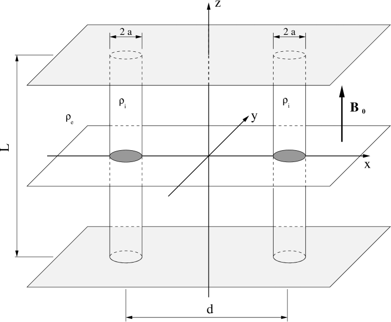
Figure 1: Sketch of the model, that consists of two straight cylinders immersed in the coronal medium. Hereafter the total pressure and the velocity fields are plotted in the $xy$-plane, shown as a white slice.

The loop centers lie on the $x$-axis at $x=d/2$ for the right loop and $x=-d/2$ for the left loop. The configuration is symmetric with respect to the $yz$-plane and the $z$-axis is parallel to the axes of the cylinders. The tubes and the environment are permeated by a uniform magnetic field along the $z$-direction ($\mathbf{B}=B_{\mathrm{0}}\mathbf{e_{\mathrm{z}}}$). The Alfvén speed, $v_{\mathrm{A}}=B_{\mathrm{0}}/\sqrt{\mu\rho}$, takes the value $v_{\mathrm{Ai}}$ inside the loop and $v_{\mathrm{Ae}}$ in the surrounding corona ($v_{\mathrm{Ai}}<v_{\mathrm{Ae}}$).

Linear perturbations about this equilibrium for a perfectly conducting fluid in the zero-$\beta$ limit can be readily described using the ideal MHD equations in Cartesian coordinates. The velocity is denoted by $\mathbf{v}=\left(v_{x},v_{y},0\right)$ and $\mathbf{B}=\left(B_{x},B_{y},B_{z}\right)$ is the magnetic field perturbation. We have assumed a $z$-dependence of the perturbations of the form $e^{-ik_{z}z}$. In this model we consider the photosphere as two infinitely dense planes located at $z=\pm L/2$. The loop feet are anchored in these planes and so the fluid velocity is zero at these positions (this is the so-called line-tying effect). This condition produces a quantization of the $z$-component of the wave-vector to $k_{z}=n\pi/L$. Hereafter we concentrate on the fundamental mode, with $n=1$. The total pressure perturbation is

$$p_{\mathrm{T}}=\frac{B_{\mathrm{0}}}{\mu}B_{z},$$ (2)

and coincides with the magnetic pressure perturbation in the zero-$\beta$ limit.

3 Normal modes

Analytical solutions to the eigenvalue problem of the previous model (assuming a temporal dependence of the form $e^{i\omega t}$) are very difficult to derive due to the geometry of the system. The methods used for a single cylinder (see Edwin and Roberts, 1983) cannot be applied to the study of two tubes. One way to solve the problem is to use scattering theory, see for example Edwin and Roberts (1983), Bogdan and Knölker (1991), Bogdan and Zweibel (1985), Bogdan and Fox (1991) and Keppens et al. (1994). Another way is to solve the eigenvalue problem given by the ideal MHD equations numerically. We have used this approach and we have done the computations with the PDE2D code (Sewell, 2005). We have used bicylindrical orthogonal coordinates, defined by the transformation

$$x=\frac{d/2\sinh v}{\cosh v-\cos u}~{},~{}y=\frac{d/2\sin u}{\cosh v-\cos u}~{},$$ (3)

where $0\leq u<2\pi$ and $-\infty<v<\infty$. The loop boundaries are coordinate surfaces at $v=\pm\mathrm{arcsinh}~{}\frac{d}{2a}$, where the positive and negative signs correspond to the right and left tubes, respectively. We impose the restriction that the solutions tend to zero at large distances from the cylinders, i.e. we seek trapped mode solutions.

We find four collective fundamental trapped modes (see Fig. 2). There are other harmonics but we concentrate on the fundamental kink-like modes because they produce the largest transverse displacement of the loops axes. The velocity field is more or less uniform in the interior of the loops, and so they move basically as a solid body, while the external velocity field has a more complex structure. The four velocity field solutions have a well defined symmetry with respect to the $y$-axis. In Figure 2a, we see that the velocity field inside the tubes lies in the $x$-direction and is symmetric with respect to the $y$-axis. We call this mode $S_{x}$, where $S$ refers to the symmetry of the velocity field and the subscript $x$ refers to the direction of the velocity inside the tube. The same nomenclature is used for the other modes. In Figure 2b the velocity inside the cylinders is mainly in the $x$-direction and antisymmetric with respect to the $y$-axis, so we call this mode $A_{x}$. Similarly, in Figure 2c the velocity lies in the $y$-direction and is symmetric with respect to the $y$-axis, while it is antisymmetric in Figure 2d. Hence, we call these modes $S_{y}$ and $A_{y}$, respectively. The pressure field of the $A_{x}$ and $S_{y}$ modes is symmetric with respect to the $y$-axis, while that of the $S_{x}$ and $A_{y}$ modes is antisymmetric.

                                                                                                                                                                                                                                                                                                     

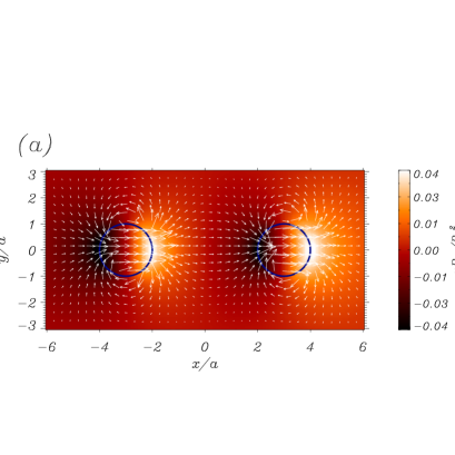
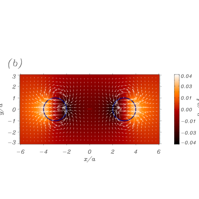
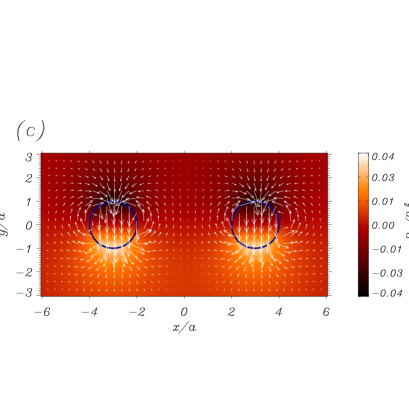
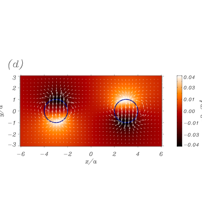
Figure 2: Total pressure perturbation (color field) and velocity field (arrows) of the fast four collective normal modes (plotted in the $xy$-plane, see Fig. 1). The modes are labeled as (a) $S_{x}$, with the loops moving in phase in the $x$-direction; (b) $A_{x}$, the tubes move in the $x$-direction but in antiphase; (c) $S_{y}$, the tubes move in the $y$-direction in phase; and finally (d) $A_{y}$, the loops move in antiphase in the $y$-direction. Here, the loop radii are $a=0.1L$ and the distance between centers is $d=6a$.

The frequencies of oscillation of these four modes as a function of the loop separation, $d$, are displayed in Figure 3. For large separations between the tubes, the modes tend to the kink mode of an individual loop (see dotted line). On the other hand, for smaller separations, they split in four branches associated to the four oscillatory modes described before. The splitting effect was noticed in Díaz et al. (2005) and Luna et al. (2006) in a configuration of several slabs. The frequency difference between the modes increases when the interaction between the loops becomes stronger, i.e. when the distance between them is small. When the loops are very close ($d\sim 2a$), the frequencies of the $S_{x}$ and $A_{y}$ modes tend to the value $\omega=3.33/\tau_{\mathrm{Ai}}$, which is similar to the internal cut-off frequency, $\omega_{\mathrm{ci}}=k_{z}v_{\mathrm{Ai}}=3.14/\tau_{\mathrm{Ai}}$ (the difference is only around 6$\%$). Here $\tau_{\mathrm{Ai}}$ is the Alfvén transit time, defined as $\tau_{\mathrm{Ai}}=L/v_{\mathrm{Ai}}$. On the other hand, in this limit, the $S_{y}$ and $A_{x}$ frequencies are quite large in comparison to the kink mode frequency.

It is interesting to note that when both tubes move symmetrically in the $x$-direction, i.e. in the $S_{x}$ mode, the fluid between follows the loops motion (see Fig. 2a). On the other hand, when the loops oscillate antisymmetrically, i.e. in the $A_{x}$ mode, the intermediate fluid is compressed and rarefied (see Fig. 2b), producing a more forced motion than that of the symmetric mode. This is the reason for the $S_{x}$ ($A_{x}$) mode having a smaller (larger) frequency than that of the individual loop. For the modes polarized in the $y$-direction the behavior is somehow similar, although in this case the antisymmetric mode (see Fig. 2d) has a lower frequency than the symmetric mode (see Fig. 2c). When one of the loops moves upwards the surrounding fluid near the other loop moves downwards. This helps to push the other loop in this direction and produces the antisymmetric motion. The situation is different for the $S_{y}$ mode, for which the direction of motion of the surrounding fluid is opposite to that of the other tube. This explains why the frequency of the $A_{y}$ solution is smaller than that of the $S_{y}$ mode.

Figure 3: Frequency, $\omega$, as a function of the separation between cylinders, $d$, for a density enhancement $\rho_{\mathrm{i}}/\rho_{\mathrm{e}}=10$ and loop radius $a=0.1L$. The lower horizontal thick dotted line is the internal cut-off frequency, $\omega_{\mathrm{ci}}=3.14/\tau_{\mathrm{Ai}}$. The thin dotted line is the kink frequency ($\omega=4.12/\tau_{\mathrm{Ai}}$) of an individual loop. The calculated frequencies from the time-dependent results in §4.1 are also plotted as triangles ($S_{x}$), squares ($A_{y}$), asterisks ($S_{y}$), and diamonds ($A_{x}$).

4 Time-dependent analysis: numerical simulations

The initial perturbation that we have used when solving numerically the ideal MHD equations is a planar pulse in the velocity field of the form

$$\mathbf{v}_{\mathrm{0}}=\mathbf{K}~{}e^{\left[-\mathbf{K}\cdot(\mathbf{r}-\mathbf{r}_{\mathrm{0}})/\Delta\right]^{2}},$$ (4)

i.e. a Gaussian profile (of width $\Delta=0.2L$ centered at $\mathbf{r}_{\mathrm{0}}=\left(d/2,0,0\right)$) and direction of propagation along $\mathbf{K}=-\left(\cos\alpha,\sin\alpha,0\right)$, $\alpha$ being the angle between the wavevector and the $x$-axis. Here $\mathbf{K}$ also defines the initial polarization of $\mathbf{v}$, which is perpendicular to the planar pulse. The initial value of the magnetic field perturbation is zero, and thus the same applies to the total pressure perturbation. In the simulations a spatial domain of size $30a\times 30a$ is used and the boundaries are far from the loops. These boundaries are open, which ensures that the numerical reflections are negligible.

In Figures 4, 5, and 6 three examples of the time evolution are shown for $\alpha=90^{\circ},0^{\circ}$ and $45^{\circ}$, respectively, and for a fixed distance between loops $d=6a$, identical to the one used in Figure 2 (see the time evolution in Movie 1, Movie 2, and Movie 3). These three cases illustrate the time evolution of the system after a perturbation, which consists of two regimes: the transient and the stationary phases. The stationary phase is characterized by oscillations in one or several fundamental trapped normal modes (see §3). On the other hand, in the transient phase there are leaky modes and internal reflections and refractions.

                                                                                                                                                                                                                                                                                                     

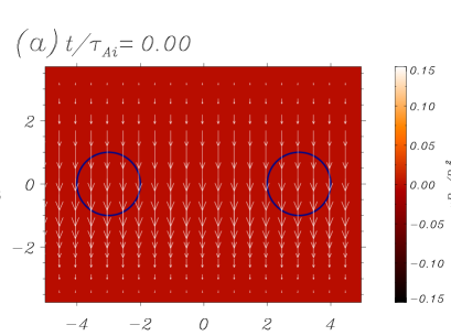
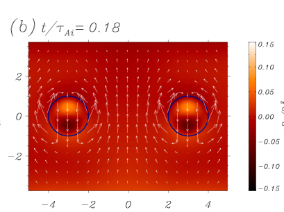
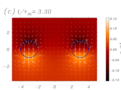
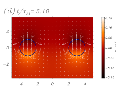
Figure 4: Time-evolution of the velocity field (arrows) and total pressure field (colored contours), for a separation between loops $d=6a$ and an initial pulse with an angle $\alpha=90^{\circ}$. The two circles mark the positions of the loops at $t=0$. The panels show different evolution times. In (a) the initial condition over the velocity field is represented. In (b) the velocity and pressure field shortly after the initial disturbance, that is, during the transient phase, are shown. Both tubes are excited at the same time. In panel (b) the tubes are in the transient phase. In panels (c) and (d) the system oscillates in the stationary phase with the $S_{y}$ normal mode. This time evolution is also available as an mpeg animation in Movie 1.

In Figure 4 (see Movie 1) the time evolution for the $\alpha=90^{\circ}$ initial disturbance is shown, for which, the pulse front lies along the $x$-axis and excites the $v_{y}$ component. The loops are perturbed at the same time (as can be appreciated in Fig. 4b) and as a consequence they oscillate symmetrically. In Figure 4b the system is in the transient phase, characterized by internal reflections related with the emission of leaky modes. The external medium has not relaxed yet. Finally, the system reaches the stationary phase (see Figs. 4c and 4d) and oscillates with the $S_{y}$ trapped mode (compare the velocity field and the pressure distribution with Fig. 2c).

                                                                                                                                                                                                                                                                                                     

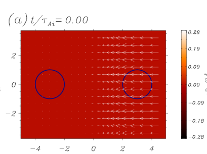
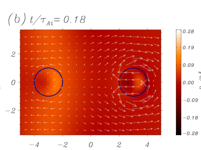
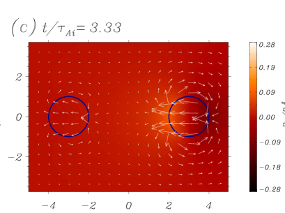
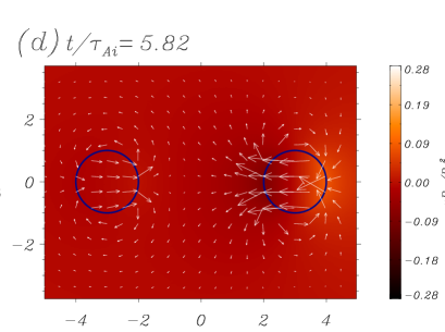
Figure 5: Same as Figure 4 for an initial pulse with an angle $\alpha=0^{\circ}$. Here the stationary phase is governed by a superposition of the $S_{x}$ and $A_{x}$ normal modes. The whole time evolution is presented in Movie 2.

In Figure 5 (and Movie 2), the time evolution for the $\alpha=0^{\circ}$ initial disturbance is shown. Now the pulse is centered on the right loop (see Fig. 5a) and excites the $v_{x}$ component. In Figure 5b, the pulse reaches the left tube and passes through it, the system still being in the transient phase. On the other hand, in Figures 5c and 5d the system oscillates in the stationary phase. It is interesting to note that this particular initial disturbance does not excite the left loop; neither at $t=0$ nor during the transient phase. Nevertheless, the oscillatory amplitude in the left loop grows with time in the stationary phase, while the amplitude in the right loop decreases in the time interval shown in Figures 5c and 5d (see also Movie 2). Then, it is clear that the left tube acquires its movement through the interaction with the right loop, i.e. by a transfer of energy from the right loop to the left loop. This process is reversed and repeated periodically: once the left loop has gained most of the energy retained by the loops system, so that the right loop is almost at rest, the left tube starts giving away its energy to the right cylinder, and so on. This is simply a beating phenomenon, that can be explained in terms of the normal modes excited in this numerical simulation. In fact, the initial disturbance excites the $S_{x}$ and $A_{x}$ modes with the same amplitude and for this reason the excitation is initially maximum on the right tube and zero on the left tube. A more detailed discussion about this issue is given in §5.

                                                                                                                                                                                                                                                                                                     

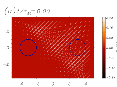
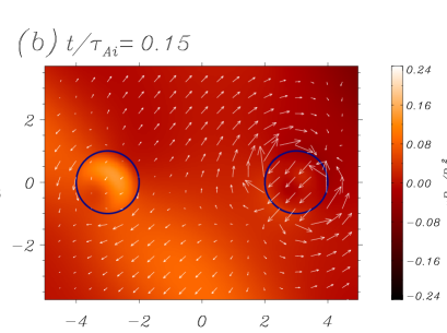
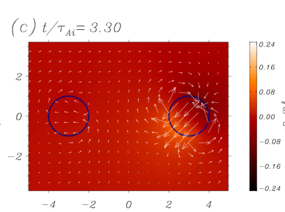
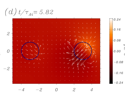
Figure 6: Same as Figure 4 for an initial pulse with an angle $\alpha=45^{\circ}$. Here the stationary phase is governed by a superposition of the $S_{x}$, $A_{x}$, $S_{y}$, and $A_{y}$ normal modes. The whole time evolution is presented in Movie 3. Movie 4 contains the time evolution for much larger times.

Finally, we discuss the results for an excitation with $\alpha=45^{\circ}$. This simulation is the most complex and general of all (see Movie 3). As we can see in Figure 6a now both components of the velocity are excited. In Figure 6b the initial pulse reaches the left tube and passes through it, but only leaky modes are excited. In Figures 6c and 6d the system oscillates in the stationary phase, which is a combination of the four modes $S_{x}$, $A_{x}$, $S_{y}$ and $A_{y}$. As in the previous case, there is beating but now it is present in both the $x$- and $y$-velocity components. Like for the previous simulation, the left loop is almost still until the stationary phase (see also dotted curves in Figs. 7a and 7d) despite that in this simulation the pulse directly hits the left loop without the obstacle of the right loop. In §5 details about the behavior of the system are given.

Once we know the general features of the excitation of the two cylinders we can perform a parametric study of the effect of the distance between the loops and also the angle of excitation on the loops motion.

4.1 Effect of the distance between loops

We generate an initial disturbance with an angle of $45^{\circ}$ for different distances $d$ and measure the velocity in the loops as a function of time. From this information we can extract the frequencies of oscillation. As we have seen, since the velocity field inside the loops is more or less uniform (see Fig. 2), it is enough to measure the velocity at the center of the loops to describe their global motion. The reason for choosing the initial disturbance with $\alpha=45^{\circ}$ is that it excites the four normal modes, so that with a single simulation we can measure their frequencies.

                                                                                                                                             

Figure 7: (a) $x$-component and (d) $y$-component of the velocity at the center of the right (solid line) and left (dotted line) loops for the numerical simulation of Figure 6 (i.e. with an initial incidence angle $\alpha=45^{\circ}$). With the method explained in §4.1 the normal mode velocities are extracted and plotted in (b) for the $S_{x}$ (solid line) and the $A_{x}$ (three-dot-dashed line) modes and in (e) for the $S_{y}$ (dashed line) and $A_{y}$ (dot-dashed line) modes. The corresponding power spectra are plotted with the same line styles in (c) and (f). Power maxima allow us to determine the frequency of the normal modes from the numerical simulation.

                                                                                                                                             

Figure 8: Same as Figure 7 for an initial incidence angle $\alpha=70^{\circ}$.

In Figures 7a and 7d the $x$- and $y$-components of the velocity at the center of each loop are plotted. In these figures we see that, after a very brief transient characterized by short-period oscillations, the system oscillates with the sum of normal modes. The frequencies of the modes are quite similar, and it is difficult to resolve them. Although the frequencies of these modes are present in the time-dependent signal, this information cannot be easily extracted from the data because in these simulations the maximum evolution time (which is determined by the numerical damping) is $T=6\tau_{\mathrm{Ai}}$. With this maximum time we have a frequency resolution $2/T\simeq 0.3/\tau_{\mathrm{Ai}}$, but, as evidenced by Figure 3, the difference in frequency between the eigenmodes is typically less than $0.1/\tau_{\mathrm{Ai}}$ so we have not enough frequency resolution. For this reason we extract the frequencies with another method considering that the velocity field is the addition of normal modes with symmetric and antisymmetric spatial functions with respect to the $y$-axis. We measure the velocity in the loop centers $(x=-d/2,y=0)$ and $(x=d/2,y=0)$, i.e. two symmetric points with respect to $x=0$. Then, the sum of both measured velocities in these points is twice the symmetric velocity. Dividing this velocity by two we obtain the $v_{x}$ of the $S_{x}$ mode and the $v_{y}$ of the $S_{y}$ mode in these points. On the other hand, the subtraction of the measured velocities is twice the antisymmetric velocity. Similarly, dividing this velocity by two we obtain the $v_{x}$ of the $A_{x}$ mode and the $v_{y}$ of the $A_{y}$ mode. The obtained mode velocities are plotted in Figures 7b and 7e. Next, we compute a periodogram of these signals (plotted in Figs. 7c and 7f), from which the frequencies of the collective modes are determined. The periodogram is preferred over the FFT as it allows to precisely identify these frequencies.

The above procedure has been applied to numerical simulations for different separations between loops and the frequencies of the four fundamental eigenmodes have been obtained. The calculated frequencies have been superimposed to the normal mode values in Figure 3 using symbols. A good agreement between the normal mode calculations and the time-dependent results can be appreciated.

4.2 Effect of the incidence angle

We next study the evolution of the system for different incidence angles, $\alpha$, of the planar pulse and a fixed distance between loops ($d=6a$). Some examples of the time evolution have already been discussed and shown in Figures 4, 5, and 6. The mode excitation depends on the width, $\Delta$, the incidence angle, $\alpha$, and the position, $\mathbf{r}_{\mathrm{0}}$, of the initial disturbance, but here we only consider the dependence on the incidence angle. The angles considered in our simulations vary from $\alpha=0^{\circ}$ to $90^{\circ}$ with steps of $5^{\circ}$. Using the method of §4.1 it is also possible to extract the amplitude of each normal mode, given by the amplitude of the sinusoidal oscillations in the stationary phase. Two examples of the extraction method are plotted in Figure 7 for $\alpha=45^{\circ}$ and Figure 8 for $\alpha=70^{\circ}$.

Figure 9: Amplitudes of the four normal modes as a function of the incidence angle $\alpha$. The separation between loops is $d=6a$.

In Figure 9 the amplitude of the four collective modes is plotted as a function of the incidence angle. The behavior of the amplitude can be divided in two parts, namely for $0^{\circ}\leq\alpha\leq 50^{\circ}$ and for $50^{\circ}<\alpha\leq 90^{\circ}$. In the first interval the amplitudes of the $S_{x}$ and $A_{x}$ modes are more or less equal (see Figs. 7b and 7e as an example) and can be approximated by $0.3\cos\alpha$. The same occurs for the amplitudes of the $S_{y}$ and $A_{y}$ modes, which vary roughly as $0.29\sin\alpha$. In the second interval these amplitudes can be quite different (see Figs. 8b and 8e as an example) and the $S_{x}$, $A_{x}$, and $A_{y}$ amplitudes go to zero at $\alpha=90^{\circ}$. On the other hand, the $S_{y}$ amplitude increases and reaches its maximum value at $\alpha=90^{\circ}$. Furthermore, for $\alpha=0^{\circ}$ the amplitudes of the $S_{x}$ and $A_{x}$ modes have a maximum around $0.3$ while the amplitudes of $S_{y}$ and $A_{y}$ modes are zero. This is because for $\alpha=0^{\circ}$ the initial disturbance drives the $x$-component of the velocity and so only the $S_{x}$ and $A_{x}$ modes are excited. Similarly, for the perturbation with $\alpha=90^{\circ}$ only the $S_{y}$ and $A_{y}$ modes can be excited, although the shape of our initial perturbation prevents the $A_{y}$ mode from being driven and so the $S_{y}$ mode reaches the largest amplitude of all modes. On the other hand, the excitation of the antisymmetric modes requires the initial disturbance to hit the right and left loops at different times. For this reason, the amplitudes of these modes decrease with $\alpha$. In fact, when $\alpha=90^{\circ}$ this time difference is zero since both loops are excited at the same time and the amplitude of the $A_{x}$ and $A_{y}$ vanishes. Finally, it is interesting to note that for $\alpha=45^{\circ}$ the four modes are excited with almost the same amplitude.

5 Study of the loops motions: beating

As we have shown in the previous section, loop motions can be very complex. This is even more clear in Movie 4, in which the time-evolution for a simulation with identical parameters to those used in Figure 6 but for much larger times is represented. In §4 we mentioned that the initial disturbance excites the right loop but does not perturb the left loop. After a short time the left tube starts to oscillate due to the interaction with the right one. At this stage, the right loop oscillates with the velocity polarization of the initial pulse, whereas the left tube oscillates in a direction perpendicular to that of the initial disturbance. The reason for the complexity of the loops motions is that their oscillations are a superposition of four normal modes with different velocity polarizations, parities, and frequencies.

Figure 10: Temporal variation of the velocity components (a) $v_{x}$ and (b) $v_{y}$ at the center of the right loop (solid line) and left loop (dashed line). These results correspond to the simulation shown in Figure 6 and illustrate the beating of the pair of loops. Damping caused by numerical dissipation causes a slight decrease of the amplitude during the numerical simulation. The time-evolution is also available as an mpeg animation in Movie 4.

We next analyze this case in detail. The $x$- and $y$-components of the velocity at the center of the loops are represented in Figures 10a and 10b, respectively. There is a clear beating, characterized by the periodic interchange of the $x$- and $y$-components of the velocity between the loops. The two velocity components are modulated in such a way that $v_{x}$ reaches its maximum value in the left tube and becomes zero in the right tube at the same time (around $t\simeq 40\tau_{\mathrm{Ai}}$). This process is reversed at $t\simeq 80\tau_{Ai}$ and repeats periodically.

The loops motions can be studied theoretically. In the stationary phase, during which the system oscillates in the normal modes $S_{x}$, $A_{x}$, $S_{y}$, and $A_{y}$, the velocity field components are

$$v_{x}(x,y,t) = C_{x}^{\mathrm{S}}(x,y)\cos\left(\omega_{x}^{\mathrm{S}}t+\phi_{x}^{S}\right)+C_{x}^{\mathrm{A}}(x,y)\cos\left(\omega_{x}^{\mathrm{A}}t+\phi_{x}^{A}\right),$$ (5)

$$v_{y}(x,y,t) = C_{y}^{\mathrm{S}}(x,y)\cos\left(\omega_{y}^{\mathrm{S}}t+\phi_{y}^{S}\right)+C_{y}^{\mathrm{A}}(x,y)\cos\left(\omega_{y}^{\mathrm{A}}t+\phi_{y}^{\mathrm{A}}\right).$$ (6)

The $\mathrm{S}$ and $\mathrm{A}$ superscripts refer to the symmetric and antisymmetric modes, respectively. The functions $C_{x}^{\mathrm{S}}$, $C_{x}^{\mathrm{A}}$, $C_{y}^{\mathrm{S}}$, and $C_{y}^{\mathrm{A}}$ represent the spatial distribution of the four normal modes (see Fig. 2) and their amplitude accounts for the energy deposited by the initial disturbance in each of them. The normal mode frequencies are represented by their frequencies, $\omega$, while $\phi$ are their initial phases.

Let us turn our attention to the results in Figure 7. In the loops centers the symmetric and antisymmetric modes have a very similar amplitude (see also Fig. 10 for $\alpha=45^{\circ}$), which means that $C_{x}^{\mathrm{S}}(d/2,0)=C_{x}^{\mathrm{A}}(d/2,0)$. Then, taking into account the parity of $C_{x}^{\mathrm{S}}$ and $C_{x}^{\mathrm{A}}$ about $x=0$, we have $C_{x}^{\mathrm{S}}(-d/2,0)=-C_{x}^{\mathrm{A}}(-d/2,0)$. Inserting these expressions into equations (5) and (6) evaluated at the loop centers we obtain

$$\mathbf{v}_{\mathrm{right}}(t) = \Big{(}C_{x}\cos(\frac{\omega_{x}^{\mathrm{A}}-\omega_{x}^{\mathrm{S}}}{2}~{}t)\cos(\frac{\omega_{x}^{\mathrm{A}}+\omega_{x}^{\mathrm{S}}}{2}~{}t),C_{y}\cos(\frac{\omega_{y}^{\mathrm{A}}-\omega_{y}^{\mathrm{S}}}{2}~{}t)\cos(\frac{\omega_{y}^{\mathrm{A}}+\omega_{y}^{\mathrm{S}}}{2}~{}t)\Big{)},$$ (7)

$$\mathbf{v}_{\mathrm{left}}(t) = -\Big{(}C_{x}\sin(\frac{\omega_{x}^{\mathrm{A}}-\omega_{x}^{\mathrm{S}}}{2}~{}t)\sin(\frac{\omega_{x}^{\mathrm{A}}+\omega_{x}^{\mathrm{S}}}{2}~{}t),C_{y}\sin(\frac{\omega_{y}^{\mathrm{A}}-\omega_{y}^{\mathrm{S}}}{2}~{}t)\sin(\frac{\omega_{y}^{\mathrm{A}}+\omega_{y}^{\mathrm{S}}}{2}~{}t)\Big{)}.$$ (8)

where $\mathbf{v}_{\mathrm{right}}$ and $\mathbf{v}_{\mathrm{left}}$ are the velocity of the right and left loop, respectively. We have defined $C_{x}=2C_{x}^{\mathrm{S}}(d/2,0)$ and $C_{y}=2C_{y}^{\mathrm{S}}(d/2,0)$ and have assumed $\phi_{x}^{\mathrm{S}}=\phi_{x}^{\mathrm{A}}=\phi_{y}^{\mathrm{S}}=\phi_{y}^{\mathrm{A}}=0$ because the initial disturbance is over the right loop. The beating curves shown in Figure 10 are accurately described by these equations.

These formulae contain products of two harmonic functions. Then, the temporal evolution during the stationary phase is governed by four periods: the two oscillatory periods,

$$T_{x}={4\pi\over\omega_{x}^{\mathrm{A}}+\omega_{x}^{\mathrm{S}}},$$ (9)

$$T_{y}={4\pi\over\omega_{y}^{\mathrm{A}}+\omega_{y}^{\mathrm{S}}},$$ (10)

giving the mean periods of the time signal; and two beating periods,

$$T_{bx}={4\pi\over\omega_{x}^{\mathrm{A}}-\omega_{x}^{\mathrm{S}}},$$ (11)

$$T_{by}={4\pi\over\omega_{y}^{\mathrm{A}}-\omega_{y}^{\mathrm{S}}}.$$ (12)

giving the periods of the envelop of the time signal. To apply these expressions to the numerical simulation of Figure 7 we insert the values of $\omega_{x}^{\mathrm{S}}$, $\omega_{x}^{\mathrm{A}}$, $\omega_{y}^{\mathrm{S}}$, and $\omega_{y}^{\mathrm{A}}$ for $d=6a$ into equations (9)–(12). Then we obtain $T_{x}=1.52\tau_{\mathrm{Ai}}$, $T_{y}=1.52\tau_{\mathrm{Ai}}$, $T_{\mathrm{b}x}=159.96\tau_{\mathrm{Ai}}$, and $T_{\mathrm{b}y}=479.88\tau_{\mathrm{Ai}}$. The two oscillating periods are equal because the frequency distribution is approximately symmetric around the central value (the kink frequency of an individual loop) for sufficiently large distances (see Fig. 3). The two beating periods derived from the numerical simulations match very well these values because Figure 10 gives $T_{\mathrm{b}x}/4\simeq 40\tau_{\mathrm{Ai}}$ and $T_{\mathrm{b}y}/4\simeq 120\tau_{\mathrm{Ai}}$.

The $\pi/2$ phase difference between $\mathbf{v}_{\mathrm{right}}$ and $\mathbf{v}_{\mathrm{left}}$ (see Figs. 7a and 7d) is due to the fact that our system of two loops basically behaves as a pair of driven-forced oscillators. Considering $v_{x}$, the left loop has initially a $\pi/2$ delay with respect to the right loop because it behaves as a driven oscillator and the left one like a forced oscillator. After half beating period, $T_{\mathrm{bx}}/2$, the roles are exchanged and left loop becomes the driver and right one the forced oscillator. The $y$-components of $\mathbf{v}_{\mathrm{right}}$ and $\mathbf{v}_{\mathrm{left}}$ exhibit the same behavior (see Fig. 7d). This was already shown by Luna et al. (2006) in the case of two slabs.

As we have seen, the polarization of the oscillations changes with time (see Movie 4 for an example). In the beating range, we can see this from the equations by calculating the scalar product of the velocity at the loop centers,

$${}\mathbf{v}_{\mathrm{right}}\cdot\mathbf{v}_{\mathrm{left}}=-C_{x}^{2}\sin\Big{(}2(\omega_{x}^{\mathrm{A}}-\omega_{x}^{\mathrm{S}})t\Big{)}\sin\Big{(}2(\omega_{x}^{\mathrm{A}}+\omega_{x}^{\mathrm{S}})t\Big{)}$$

$$-C_{y}^{2}\sin\Big{(}2(\omega_{y}^{\mathrm{A}}-\omega_{y}^{\mathrm{S}})t\Big{)}\sin\Big{(}2(\omega_{y}^{\mathrm{A}}+\omega_{y}^{\mathrm{S}})t\Big{)}.$$ (13)

This product gives the relative polarization of the loop oscillations and we see that is zero at $t=0$ and approximately zero for sufficiently small times. Thus, the left loop does not oscillate initially and it starts to oscillate perpendicularly to the right loop during the first oscillations. This feature is shown in Figure 6 and Movie 3 and Movie 4.

Similar beating features are recovered for incidence angles of the initial disturbance in the range $0^{\circ}\leq\alpha\lesssim 50^{\circ}$ (what we call the beating range). The cause of this behavior is explained by Figure 9: for these values of $\alpha$ a similar amount of energy is deposited in the $S_{x}$ and $A_{x}$ modes, so the beating of the $v_{x}$ component is possible. Obviously, an analogous argument applies to $v_{y}$. This is not the case for $50^{\circ}\lesssim\alpha\leq 90^{\circ}$ for which the symmetric and antisymmetric modes receive different amounts of energy from the initial excitation and then their relative amplitude is different (see Fig. 8 for an example). Simulations for angles $\alpha>50^{\circ}$ do not clearly exhibit beating and the trajectories of the loops are much more complex than those in the beating range.

6 Discussion and conclusions

In this work, we have investigated the transverse oscillations of a system of two coronal loops. We have considered the low-$\beta$, ideal MHD equations and have studied both the normal modes of this configuration and the time-dependent problem. The results of this work can be summarized as follows:

• The system has four fundamental normal modes, somehow similar to the kink mode of a single cylinder. These modes are collective, i.e. the system oscillates with a unique frequency, different for each mode. When arranged in increasing frequency the modes, are $S_{x}$, $A_{y}$, $S_{y}$, and $A_{x}$, where $S$($A$) stand for symmetric (antisymmetric) velocity oscillations with respect to the plane in the middle of the two loops and $x$ ($y$) stands for the polarization of motions. These modes produce transverse motions of the tubes, so they are kink-like modes.

• We have studied the eigenfrequencies as a function of the separation of loops. For large distances between cylinders, they behave as a two independent loops, i.e. the frequency tends to the individual kink mode frequency. When the distance decreases the frequency splits in four branches, two of which correspond to the $S_{x}$ and the $A_{y}$ modes and are below the frequency of the individual tube, and the other two are related to the $S_{y}$ and $A_{x}$ modes and lie above the kink frequency of a single tube. Roughly speaking, there is a certain parallelism between our system of two loops and a mechanical system of two coupled oscillators with $f$ degrees of freedom, which has $f\times n$ collective normal modes. This parallelism is possible because a slab or a cylinder oscillating with the kink mode moves more or less like a solid body. The number of translational degrees of freedom one for an individual slab ($f=1$) and two for an individual loop. Then, the parallelism with the mechanical system tells us that in a two slab system there are two collective normal modes (Luna et al., 2006), while in a two cylinder system there are four.

• For small distances between the loops, the frequency of the $S_{x}$ and $A_{y}$ modes is quite similar and tends to the internal cut-off frequency. This is different to the behavior in a configuration of two slabs (see Luna et al., 2006) where, for small distances between the slabs, the system behaves as an individual loop of double width. On the other hand, for the two cylinders the frequency is much lower than that of a loop with double radius.

• We have also studied the temporal evolution of the system after an initial planar pulse. We have shown that, depending on the incidence angle, the system oscillates with a combination of several normal modes. The frequencies of oscillation calculated from the numerical simulations agree very well with the normal mode eigenfrequencies.

• In the beating range ($0^{\circ}\leq\alpha\lesssim 50^{\circ}$), the system beats in the $x$- and $y$-components of the velocity and the left and right loops are $\pi/2$ out of phase for each velocity component. They behave as a pair of driven-forced oscillators, with one loop giving energy to the other and forcing its transverse oscillations. The role of the two loops is interchanged every half beating period. On the other hand, for perturbations with $\alpha>50^{\circ}$ the loops motions are much more complex than those in the beating range. The phase lag cannot be clearly appreciated and it strongly depends on the incidence angle of the initial pulse.

From this work, we conclude that a loop system clearly shows a collective behavior, its fundamental normal modes being quite different from the kink mode of a single loop. These collective normal modes are not a combination of individual loop modes. This suggests that the observed oscillations reported in Aschwanden et al. (1999, 2002); Schrijver et al. (2002); Verwichte et al. (2004) are in fact caused by one or a superposition of some collective modes. Moreover, the antiphase movements reported by Nakariakov et al. (1999) can be easily explained using our model. The same applies to the bounce movement of loops D and E studied in Verwichte et al. (2004). These motions can be interpreted by assuming that there is beating between the loops produced by the simultaneous excitation of the fundamental $S_{x}$ and $A_{x}$ modes.

It should be noted that the observations indicate a very rapid damping of transverse oscillations, such that in a few periods the amplitude of oscillation of the loops is almost zero. This fast attenuation may hide the beating produced by the simultaneous excitation of several normal modes of the system. However, in some situations, for example, for small loop separations and high density contrast loops, the beating periods decrease. Then, under such conditions the beating could be detectable in the observation interval. In any case, the beating is just one particular collective behavior, and there is always interaction between the individual loops in short time scales (typically of the order of $2d/v_{\mathrm{Ae}}$). The consequences of this interaction are the collective normal modes of the system. The presence of the normal modes could be also clear from a frequency analysis. Unfortunately, due to the temporal resolution, these observations do not allow us to perform such analysis, but the frequency extraction method derived in §4.1 is suitable to be applied to the observations.

Finally, in order to have more realistic models additional effects need to be included. In this work, we have studied two loops with exactly the same density and radii, so the next step is to analyze the behavior of a system of $n$ loops with different properties. This study could also be extended to understand the possible effect of internal structure (multi-stranded models and small filling factors) on the oscillating loops by considering a set of very thin tubes with different densities and radii. We expect that the dynamical behavior and frequencies of multi-stranded loops differ from those of the monolithic models. Preliminary work has been done by Arregui et al. (2007) who have studied the effects on the dynamics of the possibly unresolved internal structure of a coronal loop composed of two very close, parallel, identical coronal slabs in Cartesian geometry.

References

- Arregui et al. (2007) Arregui, I., Terradas, J., Oliver, R., & Ballester, J. L. 2007, A&A, 466, 1145
- Aschwanden et al. (1999) Aschwanden, M. J., Fletcher, L., Schrijver, C. J., & Alexander, D. 1999, ApJ, 520, 880
- Aschwanden et al. (2002) Aschwanden, M. J., De Pontieu, B., Schrijver, C. J., & Title, A. M. 2002, Sol. Phys., 206, 99
- Aschwanden et al. (2005) Aschwanden, M. J., & Nightingale, W. 2005, ApJ, 633, 499
- Berton and Heyvaerts (1987) Berton, R., & Heyvaerts, J. 1987, Sol. Phys., 109, 201
- Bogdan and Zweibel (1985) Bogdan, T. J., & Zweibel, E. G. 1985, ApJ, 298, 867
- Bogdan and Knölker (1991) Bogdan, T. J., & Knölker, M. 1990, ApJ, 369, 219
- Bogdan and Fox (1991) Bogdan, T. J., & Fox, D. C. 1991, ApJ, 379, 758
- Cally (1986) Cally, P. S. 1986, Sol. Phys., 103, 277
- DeForest (2007) DeForest, c. E. 2007, ApJ, 661, 532
- Edwin and Roberts (1983) Edwin, P. M., & Roberts, B. 1983, Sol. Phys., 88, 179
- Hudson et al. (2004) Hudson, H. S., & Warmuth, A. 2004, ApJ, 614, L85
- Díaz et al. (2005) Díaz, A. J., Oliver, R., & Ballester, J. L. 2005, A&A, 440, 1167-1175
- Keppens et al. (1994) Keppens, R., Bogdan, T. M., & Goossens, M. 1994, ApJ, 436, 372
- Klimchuk (2006) Klimchuk, J. A. 2006, Sol. Phys., 234,41
- Leveque (2002) Leveque, R. J. 2002, Finite Volume Methods for Hyperbolic Problems, Cambridge University Press
- López Fuentes et al. (2006) López Fuentes, M. C., & Klimchuk, J. A. 2006, ApJ, 639, 459
- Luna et al. (2006) Luna M., Terradas J., Oliver R., & Ballester J. L. 2006, A&A, 457, 1071-1079
- Murawski (1993) Murawski, K. 1993, Acta Astronomica, 43, 2, 161
- Murawski and Roberts (1994) Murawski, K., & Roberts, B. 1994, Sol. Phys., 151, 305
- Nakariakov et al. (1999) Nakariakov, V. M., Ofman, L., DeLuca, E. E., Roberts, B., & Davila, J. M. 1999, Science, 285, 862
- Sewell (2005) Sewell, G. 2005, The Numerical Solution of Ordinary and Partial Differential Equations, Wiley-Interscience
- Schrijver and Brown (2000) Schrijver, C. J., & Brown, D. S. 2000, ApJ, 537, L69
- Schrijver et al. (2002) Schrijver, C. J., Aschwanden, M. J., & Title, A. M. 2002, Sol. Phys., 206,69
- Spruit (1981) Spruit, H. C. 1982, Sol. Phys., 75, 3
- Terradas et al. (2005) Terradas, J., Oliver, R., & Ballester, J. L. 2005, A&A, 441, 371
- Verwichte et al. (2004) Verwichte, E., Nakariakov, V. M., Ofman, L., & Deluca, E. E. 2004, Sol. Phys., 223, 77