A cellular automaton identification of the universality classes of spatiotemporal intermittency

Abstract

The phase diagram of the coupled sine circle map lattice shows spatio-temporal intermittency of two distinct types: spatio-temporal intermittency of the directed percolation (DP) class, and spatial intermittency which does not belong to this class. These two types of behaviour are seen to be special cases of the spreading and non-spreading regimes seen in the system. In the spreading regime, each site can infect its neighbours permitting an initial disturbance to spread, whereas in the non-spreading regime no infection is possible. The two regimes are separated by a line which we call the infection line. The coupled map lattice can be mapped on to an equivalent cellular automaton which shows a transition from a probabilistic cellular automaton (PCA) to a deterministic cellular automaton (DCA) at the infection line. Thus the existence of the DP and non-DP universality classes in the same system is signalled by the PCA to DCA transition. We also discuss the dynamic origin of this transition.

The identification of the universality class of spatiotemporal intermittency daviaudpirat in spatially extended systems has been a long standing problem in the literature. Early conjectures argued that the transition to spatio-temporal intermittency is a second order phase transition, and the transition falls in the same universality class as directed percolation Pomeau . This conjecture has become the central issue in a long-standing debate Rolf ; Chate ; Grassberger , which is still not completely resolved.

Studies of the coupled sine circle map lattice have thrown up a number of intriguing observations of relevance to this problem JanZ1Z2 . This system has regimes of spatio-temporal intermittency (STI) with critical exponents which fall in the same universality class as directed percolation (DP), as well as regimes of spatial intermittency (SI) which do not belong to the DP class. Both these regimes lie on the bifurcation boundaries of the synchronised solutions of the map. The spatio-temporally intermittent regime seen here has an absorbing laminar state, i.e. a laminar site remains laminar unless infected by a neighbouring turbulent site. The burst states spread and can percolate through the entire lattice. The system shows a convincing set of directed percolation exponents in this regime JanZ1Z2 . In the spatially intermittent regime, the laminar sites are frozen in time and the burst sites show temporally periodic or quasi-periodic behaviour. The laminar sites do not get infected by neighbouring turbulent sites. Hence, the spatially intermittent state is non-spreading and does not show directed percolation exponents. Thus, both DP and non-DP behaviour can be seen for different parameter regimes of the same system.

In the present paper, we show that the infective directed percolation behaviour of spatio-temporal intermittency and the non-infective behaviour of spatial intermittency are special cases of the more general spreading to non-spreading transition seen in this system. The spreading and non-spreading regimes are separated by a line which we call the infection line. Above the infection line, the burst states can infect neighbouring laminar states and spread through the lattice, whereas below this line the burst states cannot infect their neighbours and the non-spreading regime is seen. The infection line intersects the bifurcation boundary of the synchronised solutions. Intermittent solutions are seen along this boundary, with the DP type of STI being seen above the infection line, and the non-DP SI being seen below the infection line. Spreading and non-spreading solutions are also seen off the bifurcation boundary. However, the distribution of laminar lengths shows power-law scaling only for parameter values which are very close to the bifurcation boundary, and falls off exponentially as the parameter values get more distant from the bifurcation boundary. Other exponents associated with DP behaviour are also observed only along the bifurcation boundaries. Further insights into the spreading to non-spreading transition are obtained by mapping the coupled map lattice (CML) onto a cellular automaton. The spreading to non-spreading transition seen across the infection line maps on to a transition from a probabilistic cellular automaton to a deterministic cellular automaton. Thus the change from spreading to non-spreading behaviour seen in the CML is reflected in this transition. We also provide a pointer to the dynamic origin of this transition.

Figure 1: shows the phase diagram of the CML. Spatiotemporal intermittency of the DP class is seen at the $\Diamond$-s. Spatial intermittency with quasi-periodic bursts is seen at the $\triangle$-s, SI with periodic bursts at the $\times$-s and$\ast$; STI with travelling wave laminar states and solitons at the boxes ($\Box$). The spreading and the non-spreading regimes separated by the infection line are shown. The region of cross-over from STI of the DP class (indicated by $\Diamond$-s), to SI with quasi-periodic bursts (indicated by $\triangle$-s) is shown in the inset.

The coupled sine circle map lattice studied here is known to model the mode-locking behaviour gauri2 seen in coupled oscillators, Josephson Junction arrays etc. The model is defined by the evolution equations

$$x_{i}^{t+1}=(1-\epsilon)f(x_{i}^{t})+\frac{\epsilon}{2}[f(x_{i-1}^{t})+f(x_{i+1}^{t})]\pmod{1}$$ (1)

where the index $i$ is a discrete site index which runs on a one dimensional lattice of $N$ sites, and $t$ s a discrete time index. The parameter $\epsilon$ is the strength of the coupling between the site $i$ and its two nearest neighbours. The local on-site map, $f(x)$ is the sine circle map defined as $f(x)=x+\Omega-\frac{K}{2\pi}\sin(2\pi x)$, where, $K$ is the strength of the nonlinearity and $\Omega$ is the winding number of the single sine circle map in the absence of the nonlinearity. We study the system with periodic boundary conditions in the parameter regime $0\leq\Omega\leq\frac{1}{2\pi}$ (where the single circle map has temporal period 1 solutions), $0\leq\epsilon\leq 1$ and $K=1.0$. The phase diagram of this model evolved with random initial conditions is shown in Fig. 1.

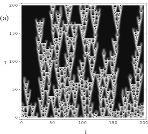
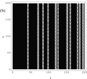
Figure 2: The space time plots of (a) STI with synchronized laminar state and turbulent bursts seen at $\Omega=0.06,\epsilon=0.7928$.(b) SI with synchronized laminar state and quasi-periodic bursts seen at $\Omega=0.031,\epsilon=0.42$.

The synchronised fixed point solutions $x^{\star}=\frac{1}{2\pi}\sin^{-1}(\frac{2\pi\Omega}{K})$ are seen in the regions indicated by dots in the phase diagram. The infection line seen in the figure separates the remaining part into the spreading and non-spreading regions. The space-time plots of the solutions seen in both these regions show co-existing laminar states and turbulent states (See Fig. 2,3).

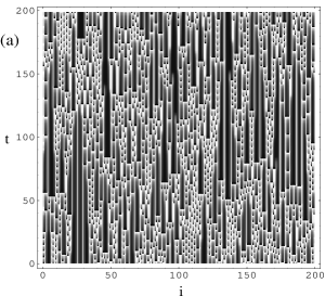
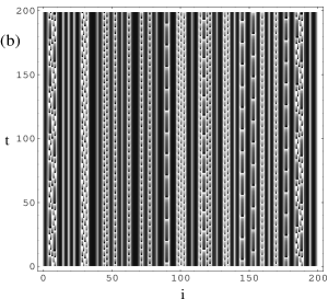
Figure 3: The space time plots seen (a) above the infection line at $\Omega=0.062,\epsilon=0.272$ and (b) below the infection line at $\Omega=0.062,\epsilon=0.258$.

The power law behaviour of the distribution of laminar lengths seen at the DP points (indicated by diamonds on the bifurcation boundary above the infection line) is shown in Fig. 4(a). This scales with an exponent $\zeta=1.67$, characteristic of directed percolation. A full set of directed percolation exponents is seen at these points JanZ1Z2 . The exponential fall off of the laminar length distributions for the spreading solutions off the bifurcation boundary, is shown in Fig. 4(b). Below the infection line, in the non-spreading regime, the laminar sites are the synchronised fixed point $x^{*}$ and the burst sites can be temporally frozen, periodic or aperiodic. The power-law scaling of the laminar length distribution for spatial intermittency is also shown in Fig. 4 (a). Here the distribution scales with exponent $\zeta=1.1$, distinct from the DP value. The exponential decrease of this distribution seen for other non-spreading solutions at points off the bifurcation boundary is shown in Fig. 4(b). Thus the sine circle map CML shows a transition from a spreading regime to a non-spreading regime. In order to gain further insights into this transition, we map the CML to a stochastic model, a probabilistic cellular automaton of the Domany-Kinzel type Chate ; domanykinzel .

Figure 4: shows the laminar length distribution of (a) STI of the DP class seen at $\Omega=0.06,\epsilon=0.7928$ and (b) SI with quasi-periodic bursts at $\Omega=0.04,\epsilon=0.402$. The data have been obtained for a $10^{4}$ site lattice and are averaged over $50$ initial conditions.

The equivalent cellular automaton, defined on a one dimensional lattice of size $N$, is set up to mimic the dynamics of the laminar and burst states. The state variable $v_{i}^{t}$ at site $i$ and at time $t$ takes values $v_{i}^{t}=0$ if the site is in the laminar state, and $v_{i}^{t}=1$ if the site is in the burst state. By the CML evolution equation (1), the state of the variable at site $i$ at time $t+1$ depends on the state of the variables at sites $i$, $i-1$ and $i+1$ at time $t$. Hence, the probability of the site $i$ at time $t+1$ being in the burst state depends on the state of the sites $i-1,i$ and $i+1$ at time $t$. We therefore define the CA dynamics in this system by the conditional probability $P(v_{i}^{t+1}|v_{i-1}^{t},v_{i}^{t},v_{i+1}^{t})$. There are $2^{3}$ possible configurations and the symmetry between the sites $i-1$ and $i+1$ in the CML equation is used to obtain the effective probabilities $p_{k}$’s, and define the CA rules as $p_{0}=P(1|000)$ , $p_{1}=P(1|001)=P(1|100)$, $p_{2}=P(1|010)$, $p_{3}=P(1|011)=P(1|110)$, $p_{4}=P(1|101)$ and $p_{5}=P(1|111)$

The direct connection between equivalent CA and the CML of eq. (1) is set up by estimating the probabilities $p_{k}$ from the numerical evolution of the CML from random initial conditions from a uniform distribution over the $(0,1)$ interval for a given set of parameter values. The probabilities are estimated by finding the fraction of sites $i$ which are in the burst state $v_{i}^{t+1}=1$ at at time $t+1$, given that the site $i$ and its nearest neighbours $i-1$ and $i+1$ existed in state $k$ at time $t$. That is, the probability $p_{k}$ is estimated using $p_{k}=\frac{N_{1}^{k}}{N_{0}^{k}+N_{1}^{k}}$, where $N_{0}^{k}$ and $N_{1}^{k}$ are the number of sites which at time $t+1$ exist in the laminar states ($v_{i}^{t+1}=0$) and the burst states ($v_{i}^{t+1}=1$) respectively and at time $t$ were the central sites of the configuration $k$. These probabilities, were extracted from a CML of size $N=2000$ averaged over $20000$ timesteps discarding a transient of $30000$ timesteps. The probabilities $p_{k}$ in the spreading and non-spreading regimes in the phase diagram are listed in the Table 1.

	$\Omega$	$\epsilon$	$p_{0}$	$p_{1}$	$p_{2}$	$p_{3}$	$p_{4}$	$p_{5}$
S(DP)	0.060	0.7928	0.0	0.220	0.0	0.933	0.627	0.984
	0.073	0.4664	0.0	0.150	0.0	0.938	0.439	0.993
S	0.070	0.264	0.0	0.140	0.0	0.982	0.391	0.999
		0.248	0.0	0.050	0.0	0.989	0.160	0.999
NS	0.070	0.232	0.0	0.000	0.0	1.000	0.000	1.000
		0.228	0.0	0.000	0.0	1.000	0.000	1.000
NS(SI)	0.031	0.420	0.0	0.000	0.0	1.000	0.000	1.000
	0.044	0.373	0.0	0.000	0.0	1.000	0.000	1.000

Table 1: shows the probabilities $p_{k}$’s obtained in the spreading (S), non-spreading (NS) regimes and at DP and SI points averaged over $50$ initial conditions.

It is clear that that the probability $p_{0}=P(1|000)$ is equal to zero in both regimes. This is the condition for an absorbing state where a laminar site with two laminar neighbours cannot spontaneously evolve into a burst state. We also see that $p_{2}=P(1|010)=0$ so that a burst site with two laminar neighbours always goes into a laminar state, i.e. the laminar neighbours suppress the central burst site. The probabilities $p_{1}=P(1|001)=P(1|100)$ and $p_{4}=P(1|101)$ are essentially infection probabilites by which a laminar site is infected by its burst neighbour or neighbours to change to a burst site.

It is clear from Table 1 that these probabilities show drastically different behaviour in the spreading and non-spreading regimes. In the case of the spatio-temporal intermittency with directed percolation exponent, which lies in the spreading regime of the phase diagram, these infection probabilities $p_{1}$ and $p_{4}$ lie in the open interval $(0,1)$. Therefore, in the spreading regime, the dynamics is described by a probabilistic cellular automaton wherein the CA rules are probabilistic in nature.

In the case of spatial intermittency which lies in the non-spreading regime, the probabilities obtained take the values $0$ or $1$. In addition to $p_{0}$ and $p_{2}$ which are zero for the STI of the DP type, the infection probabilities $p_{1}$ and $p_{4}$ go to zero, and $p_{3}=P(1|011)=P(1|110)$ and $p_{5}=P(1|111)$ take the value $1$. We also note that $p_{2}$ is zero in the non-spreading regime, as a single burst site with two laminar neighbours is never observed in the non-spreading regime. Thus the probability of infection of a laminar state by its neighbouring burst state is zero in this regime, and no spreading of bursts can occur here. Cellular automata with probabilities which take values $0$ and $1$ alone are called deterministic cellular automata (DCA), as given the state of the system at a time $t$, its state at the time $t+1$ is deterministically known. Thus the spatial intermittency in the non-spreading regime can be represented by a DCA, up to the coarse graining defined earlier. Similar behaviour, either PCA (in the spreading regime) or DCA (in the non-spreading regime), is observed at other parameter points.
A simple mean field approximation can be set up for the PCA bagnoliatman . Let $m_{t}$ and $m_{t+1}$ be the density of burst states in the lattice at the $t^{th}$ and $t+1^{th}$ timestep. Using the CA rules defined above, the mean field evolution equation for the density of bursts is given by $m_{t+1}=(2p_{1}+p_{2})m_{t}(1-m_{t})^{2}+(2p_{3}+p_{4})m_{t}^{2}(1-m_{t})+p_{5}m_{t}^{3}$.

Approximating the values of Table 1 by $p_{5}=1$, and using $p_{2}=0$, the evolution equation reduces to $m_{t+1}=2p_{1}~{}m_{t}(1-m_{t})^{2}+(2p_{3}+p_{4})~{}m_{t}^{2}(1-m_{t})+m_{t}^{3}$. This equation has three fixed points $m=0$, $m=\frac{2p_{1}-1}{1+2p_{1}-2p_{3}-p_{4}}=m^{\star}$, $m=1$.

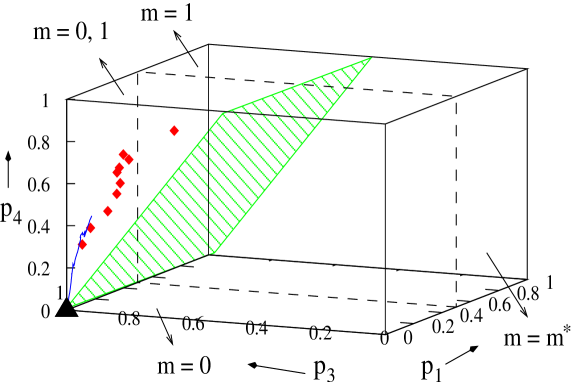
Figure 5: (Color online) shows the $\{p_{1},p_{3},p_{4}\}$ probabilities of the DP points (marked with diamonds) and for points in the spreading regime at $\Omega=0.065$ (dotted line). The triangle corresponds to the probabilities in the non-spreading regime.

The stability regions of these fixed points, as well as the co-existence region, where both the fixed points $m=0$ and $m=1$ are stable, are shown in Figure 5. The DP probabilities seen in the spreading regime, as well as the PCA probabilities seen at other points in the spreading regime, lie in this co-existence region with the $2p_{3}+p_{4}=2$ plane as a lower bound. However, all the probabilities associated with the deterministic cellular automaton seen in the non-spreading regime (i.e. $p_{1}=0,~{}p_{3}=1,~{}p_{4}=0$) lie at the vertex of the co-existence region in this cube (marked with a triangle in Fig. 5). As the parameters $\Omega$ and $\epsilon$ vary along curves which cross the infection line, the PCA probabilities seen in the spreading regime collapse to the DCA probabilities at the vertex of the cube. Thus a PCA to DCA transition occurs at the infection line. Since the DP behaviour and the spatially intermittent behaviour along the bifurcation boundaries are special cases of spreading and non-spreading behaviour, the transition from the DP universality class of spatio-temporal intermittency to the non-DP universality class of spatial intermittency is reflected in the transition from the PCA to the DCA chateca .

The dynamical reason for this transition can be found by investigating the bifurcation diagram of the system (Fig. 6). The range of $\epsilon$ values on the vertical axis of Fig. 1 cut across the infection line at $\epsilon=0.254$. The bifurcation diagram clearly shows that an attractor widening crisis greb appears at this point. Similar behavior is seen for other sites. The spreading regime seen in the phase diagram emerges exactly at the point at which the attractor widens, with the non-spreading regime corresponding to the pre-widening regime. This widening also identifies the point at which the equivalent cellular automaton undergoes a PCA to DCA transition. In the pre-crisis region, each site follows either a periodic or quasiperiodic trajectory and is not infected by the behaviour of its neighbours. Thus, its CA analogue is deterministic as listed in Table 1. In the postcrisis regime, each site is able to access the full $x$ range, as well as infect its neigbours,and the bursting and spreading behaviour characteristic of the spreading regime is seen. This is reflected in the equivalent cellular automaton by a transition to PCA behavior (Table 1). It is to be noted that the volume of the attractor in phase space will be much larger post-crisis, as compared to the pre-crisis volume. Further characterisation of the crisis is in progress.

Figure 6: shows the bifurcation diagram at $\Omega=0.065$ where $x$ values for a typical site $i$ have been plotted as a function of $\epsilon$, an initial transient of $14,000$ iterates has been discarded.

To conclude, the spatio-temporal intermittency of the directed percolation class and the spatial intermittency of the non-directed percolation class, seen along the bifurcation boundaries of synchronised solutions, are special cases of the spreading and non-spreading regimes seen off the bifurcation boundaries. The two regimes are separated by the infection line which intersects with the bifurcation boundary of the synchronised solutions at the point where the cross-over between the directed percolation and non-directed percolation behaviour takes place. Thus the behaviour seen in coupled sine circle map lattice is organised around the locations of the bifurcation boundaries and the synchronised solutions, and the infection line. The existence of two distinct universality classes, in the phase diagram of the sine circle map lattice is a reflection of the transition of the equivalent cellular automaton from the probabilistic phase to the deterministic phase and the concomitant suppression of the spreading or infectious modes. The dynamic origins of this transition lie in an attractor-widening crisis. We believe this is the first time that such a direct connection has been found between a dynamical phenomenon viz. a crisis in an extended system and the statistical properties of the extended system viz. the exponents and universality classes. Similar directed percolation to non-directed percolation transitions have been seen in other coupled map lattices, as well as in pair contact processes, solid on solid models and models of non-equilibrium wetting Odor . Our results may have useful pointers for the analysis of other systems, and thus contribute to the on-going debate on the identification of the universality classes of spatiotemporal systems.

ZJ thanks CSIR, India and NG thanks DST, India for partial support under the project SR/S2/HEP/10/2003.

References

- (1) F. Daviaud, M. Bonetti, M. Dubois, Phys. Rev. A, 42, 3388 (1990); C. Pirat, A. Naso, Jean-Louis Meunier, P. Maissa, and C. Mathis, Phys. Rev. Lett. 94, 134502 (2005); P. Rupp, R. Richter and I. Rehberg, Phys. Rev. E 67, 36209 (2003).
- (2) Y. Pomeau, Physica D 23, 3 (1986).
- (3) J. Rolf, T. Bohr, and M. H. Jensen, Phys. Rev. E 57, R2503 (1998); T. Bohr, M. van Hecke, R. Mikkelsen and M. Ipsen, Phys. Rev. Lett. 86, 5482 (2001).
- (4) H. Chaté and P. Manneville, Physica D 32, 409 (1988).
- (5) P.Grassberger and T.Schreiber, Physica D,50,177(1991).
- (6) Z. Jabeen and N. Gupte, Phys. Rev. E 74, 16210(2006), Z. Jabeen and N. Gupte, Phys. Rev. E 72, 16202(2005), T.M. Janaki, S. Sinha, and N. Gupte, Phy. Rev. E 67, 56218 (2003).
- (7) G. R. Pradhan, N. Chatterjee, and N. Gupte, Phys. Rev. E 65, 46227 (2002)
- (8) E. Domany and W.Kinzel, Phys. Rev. Lett.53,311(1984).
- (9) A similar analysis has been carried out in F. Bagnoli, N. Boccara, and R. Rechtman, Phys. Rev. E. 63, 46116 (2001).
- (10) PCA-DCA regimes have also been seen in the Chaté Manneville CML. See H. Chaté and P. Manneville, J. Stat. Phys. 56, 357 (1989).
- (11) C. Grebogi, E. Ott, F. Romeiras and J. A. Yorke, Phys. Rev. A 36, 5365 (1987).
- (12) G. Odor, Rev. Mod. Phys. 76, 663, (2004).