Fluctuation-Dissipation relations far from Equilibrium

Abstract

In this Article we review some recent progresses in the field of non-equilibrium linear response theory. We show how a generalization of the fluctuation-dissipation theorem can be derived for Markov processes, and discuss the Cugliandolo-Kurchan Cugliandolo93 fluctuation dissipation relation for aging systems and the theorem by Franz et. al. Franz98 relating static and dynamic properties. We than specialize the subject to phase-ordering systems examining the scaling properties of the linear response function and how these are determined by the behavior of topological defects. We discuss how the connection between statics and dynamics can be violated in these systems at the lower critical dimension or as due to stochastic instability.

PACS: 05.70.Ln, 75.40.Gb, 05.40.-a

I Introduction

The fluctuation-dissipation theorem Kubo (FDT) is one of the fundamental accomplishments of linear response theory applied to equilibrium systems. According to the FDT a response function $\chi$, describing the effects of a small perturbation exerted on a system, is linearly related, via the equilibrium temperature $T$, to a correlation function $C$ of the the system in the absence of the perturbation. In the language of magnetic systems, which we shall adopt in the following, one usually considers the application of an external magnetic field $h$, and $\chi$ is the magnetic susceptibility.

In recent years there has been a considerable interest, arisen in different fields such as turbulent fluids Hohenberg89 , disordered, glassy Cugliandolo93 ; Cugliandolo97 ; Berthier00 and aging systems Fielding02 , in the generalization of the results of linear response theory to out of equilibrium systems. Differently from equilibrium statistical mechanics, where a well funded and controlled theory is available, there is not nowadays a theorem of a generality comparable to the FDT for non-equilibrium states. Nevertheless, some interesting progresses have been done in understanding some particular aspects of non-equilibrium linear response theory, some of which will be discussed in this paper.

A first basic question regards the possibility of generalizing the FDT. Namely, the question is whether also away from equilibrium it is still possible to relate the response function to properties of the unperturbed dynamics, possibly in the form of correlation functions. A positive answer to this question exists when the time evolution is Markovian and described by a differential equation of the Langevin type CKP or for systems described by a master equation noialg . In this case, the response function is related to correlation functions of the unperturbed systems, which, however, are not only the correlation $C$ involved in equilibrium. These results are particularly important since they allow the study of the response function without considering the perturbed system, which is generally more complicated.

Once a relation between response and correlations is established, at least in the restricted framework of Markov processes, the natural question is which piece of information, if any, can be learned from it about the non-equilibrium state. In equilibrium the linear relation between $\chi$ and $C$ is universal, and the coefficient $d\chi/dC$ entering this relation is $T$. In the restricted area of aging systems it has been shown that the $\chi(C)$ relation still bears an universal character, although weaker than in equilibrium. This is because the theorem by Franz, Mezard, Parisi and Peliti Franz98 connects $\chi(C)$ to the equilibrium probability distribution of the overlaps $P_{eq}(q)$ and different statistical mechanical systems can be classified into few universality classes on the basis of their $P_{eq}(q)$ according to the replica symmetry breaking character of the ground state Ricci99 . Moreover, $d\chi/dC$ can be interpreted as an effective temperature Cugliandolo97 .

These results promoted linear response theory as an important tool to investigate the non-equilibrium behavior or even the structure of equilibrium states of complex systems, such as spin glasses, which are hard to equilibrate, where $P_{eq}(q)$ can be better inferred from a non-equilibrium measurement of $\chi(C)$. However, in order for these studies to be sound, a basic understanding of the out of equilibrium behavior of the response function is required. Instead, already at the level of coarsening systems, which can be considered as the simplest paradigm of aging phenomenon, where a satisfactory general analytic description can nowadays be given by means of exactly solvable models or approximate theories, the scaling properties of the response function are non trivial and still far from being understood. Notably, the statics-dynamics connection stated by the theorem Franz98 is not always fulfilled in coarsening systems.

In this paper we review some recent progresses in the field of non-equilibrium linear response theory. The focus is mainly on aging systems and, in particular, on phase-ordering, which, because of its relative simplicity, is better suited for a thorough analysis. The article is organized as follows: Secs. II, III,  IV and V are of a general character; here we fix up the basic definitions, discuss the generalization of the FDT for Markov processes, introduce the fluctuation-dissipation relation and review the theorem Franz98 which links statics to dynamics. In Sec. VI some of the concepts introduced insofar are specialized to the case of phase-ordering kinetics. After a general description of the dynamics in Sec. VI.1, the behavior of the response function is reviewed in Sec. VI.2. In particular,in Sec. VI.2.1 the scaling properties of $\chi$ are discussed and in Sec. VI.2.2 it is shown how, in the case of a scalar order parameter, the exponents can be related to the roughening properties of the interfaces. Sec. VI.3 contains a discussion of how the connection between statics and dynamics is realized or violated in coarsening systems. Some open problems are enumerated in Sec. VII and the conclusions are drawn.

II Basic Definitions

Let us consider a system described by the Hamiltonian $H_{0}$. The autocorrelation function of a generic observable ${\cal O}$ between the two times $s$ and $t\geq s$ is

$$C(t,s)=\langle{\cal O}(t){\cal O}(s)\rangle,$$ (1)

where $\langle\dots\rangle$ is an ensemble average. Switching on an impulsive perturbation $h(s)$ at time $s$ which changes the Hamiltonian ${\cal H}\to{\cal H}+\Delta{\cal H}={\cal H}-h{\cal O}$, the linear (impulsive) response function is given by

$$R(t,s)=\left.\frac{\partial\langle{\cal O}(t)\rangle}{\partial h(s)}\right|_{h=0}$$ (2)

The integrated response function, or dynamic susceptibility, is

$$\chi(t,s)=\int_{s}^{t}R(t,t^{\prime})dt^{\prime}$$ (3)

and corresponds to the response to a perturbation switched on from $s$ onwards.

In equilibrium, time translation invariance (TTI) holds, so that all the two time quantities introduced above depend only on the time difference $\tau=t-s$. The FDT reads

$$TR(\tau)=-\frac{dC(\tau)}{d\tau},$$ (4)

where $T$ is the temperature, or, equivalently, for the integrated response

$$T\chi(\tau)=C(\tau=0)-C(\tau).$$ (5)

III Off-equilibrium generalization of the fluctuation dissipation theorem for Markov processes

Consider a system with an order parameter field $\phi(\vec{x})$ evolving with the Langevin equation of motion

$${\partial\phi(\vec{x},t)\over\partial t}=B\left[\phi(\vec{x},t)\right]+\eta(\vec{x},t)$$ (6)

where $B\left[\phi(\vec{x},t)\right]$ is the deterministic force and $\eta(\vec{x},t)$ is a white, zero-mean Gaussian noise. In this framework a generalization of the FDT was derived in CKP . Let us recall the basic elements, referring to CKP for further details. From Eq. (6), the linear response function is simply computed as the correlation function of the order parameter with the noise

$$2TR(t,s)=\langle\phi(\vec{x},t)\eta(\vec{x},s)\rangle$$ (7)

where $T$ is the temperature of the thermal bath and $t\geq s$ by causality. It is straightforward to recast the above relation in the form

$$TR(t,s)=\frac{1}{2}\frac{\partial C(t,s)}{\partial s}-\frac{1}{2}\frac{\partial C(t,s)}{\partial t}-A(t,s)$$ (8)

where

$$C(t,s)=\langle\phi(\vec{x},t)\phi(\vec{x},s)\rangle-\langle\phi(\vec{x},t)\rangle\langle\phi(\vec{x},s)\rangle$$ (9)

and

$$A(t,s)\equiv\frac{1}{2}\left\{\langle\phi(\vec{x},t)B\left[\phi(\vec{x},s)\right]\rangle-\langle B\left[\phi(\vec{x},t)\right]\phi(\vec{x},s)\rangle\right\}$$ (10)

is the so called asymmetry. Eq. (8), or (7), qualifies as an extension of the FDT out of equilibrium, since in the right hand side there appear unperturbed correlation functions. When time translation and time inversion invariance hold, so that $A(t,s)=0$ and $\partial C(t,s)/\partial t=-\partial C(t,s)/\partial s$, it reduces to the equilibrium FDT (4). Let us mention that this equation holds noialg in the same form both for conserved order parameter (COP) and non conserved order parameter (NCOP) dynamics Bray94 .

The next interesting question is whether one can do the same also in the case of discrete spin variables, where the kinetics is described by a master-equation, there is no stochastic differential equation and, therefore, Eq. (7) is not available. A first approach to this problem was undertaken in Refs. chat ; ricci ; diez ; Crisanti2002 where a relation between the response function and particular correlators was obtained. As we shall discuss briefly below, however, their results cannot be qualified as generalizations of the fluctuation-dissipation theorem. Instead, in what follows we scketch how (details can be found in noialg ), an off- equilibrium generalization of the FDT, which takes exactly the same form as Eqs. (8,10) and which holds, as in the Langevin case, for NCOP (spin flip) and COP (spin exchange) dynamics can be derived also in this case.

Let us consider a system of Ising spins $\sigma_{i}=\pm 1$ executing a Markovian stochastic process. The generalization to $q$-states spins, as in the Potts or Clock model, is straightforward. The problem is to compute the linear response $R(t,s)$ on the spin at the site $i$ and at the time $t$, due to an impulse of external field at an earlier time $s$ and at the same site $i$. Let

$$h_{j}(t)=h\delta_{i,j}\theta(t-s)\theta(s+\Delta t-t)$$ (11)

be the magnetic field on the $i$-th site acting during the time interval $[s,s+\Delta t]$, where $\theta$ is the Heavyside step function. The response function then is given by chat ; Crisanti2002

$$R(t,s)=\lim_{\Delta t\to 0}\frac{1}{\Delta t}\left.\frac{\partial\langle\sigma_{i}(t)\rangle}{\partial h_{j}(s)}\right|_{h=0}$$ (12)

where

$$\left.\frac{\partial\langle\sigma_{i}(t)\rangle}{\partial h_{j}(s)}\right|_{h=0}=\sum_{[\sigma],[\sigma^{\prime}],[\sigma^{\prime\prime}]}\sigma_{i}p([\sigma],t|[\sigma^{\prime}],s+\Delta t)\left.\frac{\partial p^{h}([\sigma^{\prime}],s+\Delta t|[\sigma^{\prime\prime}],s)}{\partial h_{j}}\right|_{h=0}p([\sigma^{\prime\prime}],s)$$ (13)

and $[\sigma]$ are spin configurations.

Let us concentrate on the factor containing the conditional probability in the presence of the external field $p^{h}([\sigma^{\prime}],s+\Delta t|[\sigma^{\prime\prime}],s)$. In general, the conditional probability for $\Delta t$ sufficiently small is given by

$$p([\sigma],t+\Delta t|[\sigma^{\prime}],t)=\delta_{[\sigma],[\sigma^{\prime}]}+w([\sigma^{\prime}]\to[\sigma])\Delta t+{\cal O}(\Delta t^{2}),$$ (14)

where we have used the boundary condition $p([\sigma],t|[\sigma^{\prime}],t)=\delta_{[\sigma],[\sigma^{\prime}]}$. Furthermore, the transition rates must verify detailed balance

$$w([\sigma]\to[\sigma^{\prime}])\exp(-{\cal H}[\sigma]/T)=w([\sigma^{\prime}]\to[\sigma])\exp(-{\cal H}[\sigma^{\prime}]/T),$$ (15)

where ${\cal H}[\sigma]$ is the Hamiltonian of the system.

Introducing the perturbing field as an extra term $\Delta{\cal H}[\sigma]=-\sigma_{j}h_{j}$ in the Hamiltonian, to linear order in $h$ the most general form of the perturbed transition rates $w^{h}([\sigma]\to[\sigma^{\prime}])$ compatible with the detailed balance condition is

$$w^{h}([\sigma]\to[\sigma^{\prime}])=w^{0}([\sigma]\to[\sigma^{\prime}])\left\{1-\frac{1}{2T}h_{j}(\sigma_{j}-\sigma^{\prime}_{j})+M([\sigma],[\sigma^{\prime}])\right\},$$ (16)

where $M([\sigma],[\sigma^{\prime}])$ is an arbitrary function of order $h/T$ symmetric with respect to the exchange $[\sigma]\leftrightarrow[\sigma^{\prime}]$, and $w^{0}([\sigma]\to[\sigma^{\prime}])$ are unspecified unperturbed transition rates, which satisfy detailed balance. In the following, for simplicity, we shall take $M([\sigma],[\sigma^{\prime}])=0$. Implication of this choice, which corresponds to a specification of the perturbed transition rates, are discussed in noialg .

Inserting Eqs. (14), (16) in Eq. (13), and using the time translational invariance of the conditional probability $p([\sigma],t|[\sigma^{\prime}],s+\Delta t)=p([\sigma],t-\Delta t|[\sigma^{\prime}],s)$, after some manipulations the response function (12) can be written as

$$TR(t,s)=\frac{1}{2}\frac{\partial C(t,s)}{\partial s}-\frac{1}{2}E(t,s)$$ (17)

where

$$C(t,s)=\langle\sigma_{i}(t)\sigma_{i}(s)\rangle$$ (18)

is the autocorrelation function,

$$E(t,s)=\langle\sigma_{i}(t)B_{i}(s)\rangle,$$ (19)

and

$$B_{i}=-\sum_{[\sigma^{\prime\prime}]}(\sigma_{i}-\sigma^{\prime\prime}_{j})w^{0}([\sigma]\to[\sigma^{\prime\prime}]).$$ (20)

For the dynamic susceptibility one has

$$T\chi(t,s)=\frac{1}{2}[C(t,t)-C(t,s)]-\frac{1}{2}\int_{s}^{t}E(t,t^{\prime})dt^{\prime},$$ (21)

It is interesting to observe that Eq. (17) is completely analogous to Eqs. (8) and (10). In fact, it can be easily shown that

$$\frac{d\langle\sigma_{i}(t)\rangle}{dt}=\langle B_{i}(t)\rangle,$$ (22)

and that

$$\frac{\partial C(t,s)}{\partial t}-\langle B_{i}(t)\sigma_{i}(s)\rangle=0.$$ (23)

Subtracting this from Eq. (17) we finally arrive at Eq. (8) where $A(t,s)$ is given by

$$A(t,s)=\frac{1}{2}\left[\langle\sigma_{i}(t)B_{i}(s)\rangle-\langle B_{i}(t)\sigma_{i}(s)\rangle\right].$$ (24)

Eqs. (8) and (24) are the main result of this Section. They are identical to Eqs. (8) and (10) for Langevin dynamics, since the observable $B$ entering in the asymmetries (10) and (24) plays the same role in the two cases. In fact, Eq. (22) is the analogous of

$${\partial\langle\phi(\vec{x},t)\rangle\over\partial t}=\langle B\left[\phi(\vec{x},t)\right]\rangle$$ (25)

obtained from Eq. (6) after averaging over the noise.

In summary, Eq. (8) is a relation between the response function and correlation functions of the unperturbed kinetics, which generalizes the FDT. Eq. (8) applies to a wide class of systems: Besides being obeyed by soft and hard spins, it holds both for COP and NCOP dynamics. Moreover, as it is clear by its derivation, it does not require any particular assumption on the Hamiltonian nor on the form of the unperturbed transition rates, and can be easily generalized nat to intrinsically non-equilibrium systems where the transition rates do not obey detailed balance. Finally, let us briefly discuss (for details see Ref. noialg ) the differences between the results discussed insofar and those obtained by Chatelain chat , Ricci-Tersenghi ricci , Diezemann diez and Crisanti and Ritort Crisanti2002 . Also in these papers, in fact, the response function is related to unperturbed correlation functions but, differently from those appairing in Eqs. (17,21), these functions must be computed on a system which evolves with an ad hoc kinetic rule, different from that of the original unperturbed system, which is introduced with the sole purpose of evaluating the response function. It can be shown that this corresponds, in the averaging procedure, to consider only a subset of trajectories of the original unperturbed system. Therefore, although the results of Refs. chat ; ricci ; diez ; Crisanti2002 are important, both for computational and analytical calculations, they cannot be regarded as generalizations of the FDT in the sense of Eq. (8) because the response function is not related to correlation functions of the unperturbed system.

IV Fluctuation dissipation relation

In the previous Section we have shown that in the cases considered the integrated response function out of equilibrium is not only related to the autocorrelation function but also to the correlation $E(t,s)$ by means of Eq. (21). A very useful tool for the study of slow relaxation phenomena has been introduced by Cugliandolo and Kurchan Cugliandolo93 through the off- equilibrium fluctuation dissipation relation (FDR). This was introduced as a direct relation between $\chi(t,s)$ and $C(t,s)$ as follows: Given that $C(t,s)$ is a monotonously decreasing function of $t$, for fixed $s$ it is possible to invert it and write

$$\chi(t,s)=\widetilde{\chi}(C(t,s),s).$$ (26)

Then, if for a fixed value of $C(t,s)$ there exists the limit

$$\lim_{s\rightarrow\infty}\widetilde{\chi}(C,s)=S(C)$$ (27)

the function $S(C)$ gives the fluctuation dissipation relation. In the particular case of equilibrium dynamics, FDT is recovered and $S(C)=[C(\tau=0)-C]/T$. Originally introduced in the study of the low temperature phase of spin glass mean-field models, the fluctuation dissipation relation has been found in many other instances of slow relaxation Crisanti2002 .

V Statics from dynamics

One of the main reasons of interest in the fluctuation dissipation relation is that it may provide a link between dynamic and static properties, and in particular with the equilibrium overlap probability function

$$P(q)=\frac{1}{Z^{2}}\sum_{[\sigma],\sigma^{\prime}]}\exp\left\{-\frac{1}{T}\left[H([\sigma])+H([\sigma^{\prime}])\right]\right\}\delta\left(Q([\sigma],[\sigma^{\prime}])-q\right)$$ (28)

where $Z$ is the partition function and $Q([\sigma],[\sigma^{\prime}])=1/N\sum_{i}\sigma_{i}\sigma_{i}^{\prime}$ is the overlap between two configurations $[\sigma]$ and $[\sigma^{\prime}]$. For slowly relaxing systems this is established in general by a theorem by Franz et al. Franz98 stating that

1. if $S(C)$ exists

2. if $\lim_{t\rightarrow\infty}\chi(t,s)=\chi_{eq}$, $\chi_{eq}$ being the equilibrium susceptibility

then the off-equilibrium fluctuation dissipation relation can be connected to equilibrium properties through

$$\left.-T\frac{d^{2}S(C)}{dC^{2}}\right|_{C=q}=\widetilde{P}(q),$$ (29)

where $\widetilde{P}(q)$ is the overlap probability function in the equilibrium state obtained in the limit in which the perturbation responsible of $\chi(t,s)$ is made to vanish. The relation between $\widetilde{P}(q)$ and the unperturbed overlap function $P(q)$ must be considered carefully. This implies the notion of stocastic stability Guerra . In a stochastically stable system the equilibrium state in the presence of a perturbation, in the limit of a vanishing perturbation, is the same as that of the corresponding unperturbed system. Notice that, while stochastic stability is always expected for ergodic systems, this property is far from being trivial when more ergodic components are present, as it is easily understood by considering the Ising model perturbed by an external magnetic field. If a system is stochastically stable then $P(q)=\widetilde{P}(q)$. A milder statement of stochastic stability is that $\widetilde{P}(q)$ coincides with $P(q)$ up to the effects of a global symmetry which might be removed by the perturbation. For instance, in the Ising case, where the perturbation breaks the up-down symmetry, defining

$$\widehat{P}(q)=2\theta(q)P(q)$$ (30)

the system is stochastically stable in the sense that $\widetilde{P}(q)=\widehat{P}(q)$. In conclusion, if the system is stochastically stable Eq. (29) holds with $\widehat{P}(q)$ on the right hand side, establishing a connection between the FDR and the equilibrium properties of the unperturbed state. On the other hand, if the system is not stochastically stable, $\widetilde{P}(q)$ is not related neither to $P(q)$ nor to $\widehat{P}(q)$. As we shall see in Sec. VI.3.2, this is the case of the mean spherical model.

With this link between statics and dynamics one can translate Ricci99 to the dynamics the usual classification of complex systems based on the kind of replica symmetry breaking Mezard87 . According to this categorization a first class of systems are those whose low temperature phase is characterized by two pure state which are related by a global spin inversion. As will be discussed in Sec. VI.3, these systems without replica symmetry breaking are described by a $\widetilde{P}(q)$ with a single $\delta$-function centered on the Edwards-Anderson order parameter $q_{EA}$ (the squared magnetization, in ferromagnetic systems), and their FDR, according to Eq. (29) is a broken line with an horizontal part. This situation is shown in Fig. 1, upper part (I). A second class of system are those where a transition with a single step of replica symmetry breaking occurs, as $p$-spins with $p>2$ in mean field, binary mixtures of soft spheres Parisi99 or Lennard-Jones mixtures Barrat99 . In these systems $\widetilde{P}(q)$ is made of two $\delta$-functions, one centered in the origin and the other around a finite $q_{EA}$. Their FDR is made of two straight lines with finite slopes, as shown in Fig. 1 in the central panel (II). Systems as the Edwards-Anderson model in mean field fall into a third category, for which $\widetilde{P}(q)$ is different from zero in a whole range $q\in[0,q_{EA}]$ with a delta function on $q_{EA}$. These systems have a FDR with a straight line and a bending curve, as shown in Fig. 1, lower part (III).

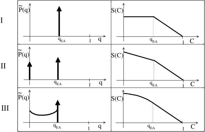
Figure 1: Classification of systems according to their $\widetilde{P}(q)$ (left) or, equivalently, on $S(C)$ (right), following ref. Ricci99 . Bold arrows represent $\delta$ functions. Rows denoted as I, II, and III describe the three classes of systems discussed in the text.

VI Phase ordering

Phase ordering Bray94 is usually regarded as the simplest instance of slow relaxation, where concepts like scaling and aging, which are the hallmarks of glassy behavior Cugliandolo2002 , can be more easily investigated. However, next to the similarities there are also fundamental differences CCY which require to keep phase ordering well distinct from the out of equilibrium behavior in glassy systems, both disordered and non disordered. The main source of the differences is the simplicity of the free energy landscape in the case of phase ordering compared to the complexity underlying glassy behavior.

Besides the obvious motivation that the basic, paradigmatic cases need to be thoroughly understood, an additional reason for studying phase ordering, among others, is that in some cases the existence of complex slow relaxation is identified through the exclusion of coarsening. An example comes from the long standing controversy about the nature of the low temperature phase of finite dimensional spin glasses. One argument in favor of replica symmetry breaking is that the observed behavior of the response function is incompatible with coarsening Franz98 ; Ricci99 . This might well be the case; however, for the argument to be sound, the understanding of the out of equilibrium behavior of the response function during phase ordering needs to be up to the level that such a delicate issue demands.

In this Section we present an overview of the accurate investigation of the response function in phase ordering that we have carried out in the last few years. Focusing on the integrated response function (3), or zero field cooled magnetization (ZFC) in the language of magnetic systems, it will be argued that the response function in phase ordering systems is not as trivial as it is believed to be and, after all, it is not the quantity best suited to highlight the differences between systems with and without replica symmetry breaking. In fact, as discussed in Secs. VI.3,VI.3.2, there are cases in which phase ordering, and therefore a replica symmetric low temperature state, are compatible with a non trivial ZFC. When this happens there is no connection between static and dynamic properties. Phase ordering systems offer examples of two distinct mechanism for the lack of this important feature of slow relaxing systems, stochastic instability and the vanishing of the scaling exponent of ZFC.

Let us first briefly recall the main features of a phase ordering process. Consider a system, like a ferromagnet, with order parameter (vector or scalar, continuous or discrete) $\phi(\vec{x})$ and Hamiltonian ${\cal H}[\phi(\vec{x})]$ such that below the critical temperature $T_{C}$ the structure of the equilibrium state is simple. For example, in the scalar case, there are two pure ordered states connected by inversion symmetry. The form of the Hamiltonian can be taken the simplest compatible with such a structure, like Ginzburg-Landau-Wilson for continuous spins or the nearest neighbors Ising Hamiltonian for discrete spins.

Let us generalize the definition (9) to the space and time dependent correlation function

$$C(\vec{r},t,s)=\langle\phi(\vec{x},t)\phi(\vec{x}^{\prime},s)\rangle-\langle\phi(\vec{x},t)\rangle\langle\phi(\vec{x}^{\prime},s)\rangle$$ (31)

where the average is taken over initial condition and thermal noise, and $\vec{r}=\vec{x}-\vec{x^{\prime}}$. We use the notation $C(\vec{r}=0,t,s)=C(t,s)$, and similarly for the response functions defined below. The linear response function conjugated to $C(\vec{r},t,s)$ is given by

$$R(\vec{r},t,s)=\left.\frac{\delta\langle\phi(\vec{x},t)\rangle}{\delta h(\vec{x^{\prime}},s)}\right|_{h=0},$$ (32)

where $h(\vec{x},t)$ is a space-time dependent external magnetic field and the integrated response function is defined by

$$\chi(\vec{r},t,s)=\int_{s}^{t}dsR(\vec{r},t,s).$$ (33)

VI.1 Dynamics over phase space: equilibration versus falling out of equilibrium

For a temperature $T$ below $T_{C}$, in the thermodynamic limit, the phase space $\Omega=\{[\phi(\vec{x})]\}$ may be regarded as the union of three ergodic components Palmer $\Omega=\Omega_{+}\cup\Omega_{-}\cup\Omega_{0}$, where $\Omega_{\pm}$ and $\Omega_{0}$ are the subsets of configurations with magnetization $\lim_{V\rightarrow\infty}\frac{1}{V}\int_{V}d\vec{x}\phi(\vec{x})$ positive, negative and vanishing, respectively. Denoting by $\rho_{\pm}[\phi(\vec{x})]$ the two broken symmetry pure states, whose typical configurations are schematically represented in Fig. 2, all equilibrium states are the convex linear combinations of $\rho_{\pm}$. In particular, the Gibbs state is the symmetric mixture $\rho_{G}[\phi(\vec{x})]=\frac{1}{Z}\exp(-{\cal H}[\phi(\vec{x})]/T)=\frac{1}{2}\rho_{+}[\phi(\vec{x})]+\frac{1}{2}\rho_{-}[\phi(\vec{x})]$. The $\Omega_{\pm}$ components are the domains of attraction of the pure states with $\rho_{+}(\Omega_{+})=\rho_{-}(\Omega_{-})=1$ and $\Omega_{0}$ is the border in between them, with zero measure in any of the equilibrium states.

When ergodicity is broken, quite different behaviors may arise Palmer depending on the initial condition $\rho_{0}[\phi(\vec{x})]=\rho([\phi(\vec{x})],t=0)$. Here, we consider the three cases relevant for what follows, assuming that there are not explicit symmetry breaking terms in the equation of motion:

1. equilibration to a pure state

   if $\rho_{0}(\Omega_{+})=1$ or $\rho_{0}(\Omega_{-})=1$, in the time evolution configurations are sampled from either one of $\Omega_{\pm}$ and $\rho([\phi(\vec{x})],t)$ equilibrates to the time independent pure state $\rho_{\pm}[\phi(\vec{x})]$ within the finite relaxation time $t_{eq}\sim\xi^{z}$, where $\xi$ is the equilibrium correlation length and $z$ is the dynamic exponent. The correlation function is the same in the two ergodic components and, after equilibration, is time translation invariant

   $$C_{st}(\vec{r},\tau)=\langle\phi(\vec{x},t)\phi(\vec{x}^{\prime},s)\rangle_{\pm}-M^{2}$$ (34)

   where $\langle\phi(\vec{x})\rangle_{\pm}=\pm M$ is the spontaneous magnetization. For large distances $r\gg\xi$ and time separations $t-s\gg t_{eq}$, the clustering property $\langle\phi(\vec{x},t)\phi(\vec{x}^{\prime},s)\rangle_{\pm}$ $=\langle\phi(\vec{x},t)\rangle_{\pm}\langle\phi(\vec{x}^{\prime},s)\rangle_{\pm}$ is obeyed and the correlations decay to zero, as required by ergodicity (see Fig. 6).

   

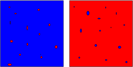
   Figure 2: Typical configurations of a binary system after equilibration to the pure states $\rho_{+}[\phi(\vec{x})]$ or $\rho_{-}[\phi(\vec{x})]$ (left and right panel).

2. equilibration to the Gibbs state

   if $\rho_{0}(\Omega_{+})=\rho_{0}(\Omega_{-})=1/2$, then configurations are sampled evenly from both disjoint components $\Omega_{+}$ and $\Omega_{-}$. The probability density $\rho([\phi(\vec{x})],t)$ equilibrates now to the Gibbs state $\rho_{G}[\phi(\vec{x})]$ with the same relaxation time $t_{eq}$ as in the relaxation to the pure states. Broken ergodicity shows up in the large distance and in the large time properties of the correlation function. After equilibration, one has

   $$C_{G}(\vec{r},\tau)=C_{st}(\vec{r},\tau)+M^{2}$$ (35)

   from which follows that correlations do not vanish asymptotically or that the clustering property is not obeyed

   $$\lim_{r\rightarrow\infty}C_{G}(\vec{r},\tau)=\lim_{\tau\rightarrow\infty}C_{G}(\vec{r},\tau)=M^{2}.$$ (36)

3. falling out of equilibrium over the border Laloux ; Newman

   If $\rho_{0}(\Omega_{0})=1$, for the infinite system $\rho(\Omega_{0},t)=1$ also at any finite time after the quench. Namely, the system does not equilibrate since in any equilibrium state the measure of $\Omega_{0}$ vanishes. Phase ordering corresponds to this case. In fact, the system is initially prepared in equilibrium at very high temperature (for simplicity $T_{I}=\infty$) and at the time $t=0$ is suddenly quenched to a final temperature $T$ below $T_{C}$. In the initial state the probability measure over phase space is uniform $\rho_{0}[\phi(\vec{x})]=1/|\Omega|$, implying that the initial configuration at $t=0$ belongs almost certainly to $\Omega_{0}$, since with a flat measure $|\Omega_{0}|$ is overwhelmingly larger than $|\Omega_{\pm}|$.

   The morphology of typical configurations visited as the system moves over $\Omega_{0}$ is a patchwork of domains of the two competing equilibrium phases, which coarsen as the time goes on, as schematically shown in Fig. 3. The typical size of domains grows with the power law $L(t)\sim t^{1/z}$, where $z=2$ (independent of dimensionality) for dynamics with non conserved order parameter Bray94 , as it will be considered here. The sampling of configurations of this type is responsible of the peculiar features of phase ordering. At a given time $s$ there remains defined a length $L(s)$ such that for space separations $r\ll L(s)$ or for time separations $t-s\ll s$ intra-domains properties are probed. Then, everything goes as in the case 2 of the equilibration to the Gibbs state, ergodicity looks broken and the correlation function obeys Eq. (35). Conversely, for $r\gg L(s)$ or $t/s\gg 1$, inter-domains properties are probed, ergodicity is restored (as it should be, since evolution takes place within the single ergodic component $\Omega_{0}$) and eventually the correlation function decays to zero. However, the peculiarity is that if the limit $s\rightarrow\infty$ is taken before $r\rightarrow\infty$, in the space sector ergodicity remains broken giving rise, for instance, to the growth of the Bragg peak in the equal time structure factor.

   

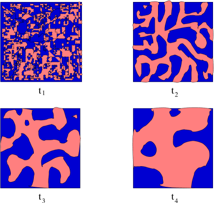
   Figure 3: Configurations of a coarsening system at different times $t_{1}<t_{2}<t_{3}<t_{4}$.

   According to this picture, the correlation function can be written as the sum of two contributions

   $$C(\vec{r},t,s)=C_{st}(\vec{r},\tau)+C_{ag}(\vec{r},t,s)$$ (37)

   where the first one is the stationary contribution of Eq. (34) describing equilibrium fluctuations in the pure states and the second one contains all the out of equilibrium information. The latter one is the correlation function of interest in the theory of phase ordering where, in order to isolate it, zero temperature quenches are usually considered as a device to eliminate the stationary component. It is now well established that $C_{ag}(\vec{r},t,s)$ obeys scaling in the form Furukawa

   $$C_{ag}(\vec{r},t,s)=\widehat{C}(r/L(s),t/s)$$ (38)

   with $\widehat{C}(x,y)=M^{2}$ for $x<1$ and $y\sim 1$, while

   $$\widehat{C}(r/L(s),t/s)\sim(t/s)^{-\lambda/z}h(r/L(s))$$ (39)

   for large time separation Bray94 , where $\lambda$ is the Fisher–Huse exponent.

VI.2 Zero field cooled magnetization

Let us next consider what happens when a time independent external field $h(\vec{x},s)$ is switched on at the time $s$. To linear order the expectation value of the order parameter at the later time $t$ is given by

$$\langle\phi(\vec{x},t)\rangle_{h}=\langle\phi(\vec{x},t)\rangle_{0}+\int d\vec{x^{\prime}}\int dsR(\vec{x}-\vec{x^{\prime}},t,s)h(\vec{x^{\prime}},s)$$ (40)

If $h(\vec{x},s)=h(\vec{x})\theta(t-s)$ is a random field switched on and kept constant from $s$ onwards, with expectations

$$\overline{h(\vec{x})}=0$$ (41)

$$\overline{h(\vec{x})h(\vec{x^{\prime}})}=h^{2}\delta(\vec{x}-\vec{x^{\prime}})$$ (42)

then one has

$$\chi(\vec{x}-\vec{y},t,s)=h^{-2}\overline{\langle\phi(\vec{x},t)\rangle_{h}h(\vec{y})}.$$ (43)

Namely, ZFC is the correlation at the time $t$ of the order parameter with the random external field.

Going to the three processes considered above, and restricting attention from now on, for simplicity, to the case of coincident points ($\vec{r}=0$)

1. after equilibration in the pure state has occurred and the stationary regime has been entered, the order parameter correlates with the external field via the equilibrium thermal fluctuations, FDT is obeyed

   $$\chi_{st}(\tau)=\frac{1}{T}\left[C_{st}(\tau=0)-C_{st}(\tau)\right]$$ (44)

   and since $C_{st}(\tau)$ decays to zero for $\tau>t_{eq}$, over the same time scale $\chi_{st}(\tau)$ saturates to

   $$\lim_{t\rightarrow\infty}\chi_{st}(\tau)=\chi_{eq}=\frac{1}{T}C_{eq}$$ (45)

   which is the susceptibility computed in the final equilibrium state $\rho_{\pm}[\phi(\vec{x})]$ (see Fig. 6).

2. As far as ZFC is concerned, there is no difference between the relaxation to the mixed Gibbs state and the relaxation to a pure state. Hence, FDT is satisfied and can be written both in terms of $C_{st}$ or $C_{G}$ since, as Eq. (35) shows, they differ by a constant.

3. In the phase ordering process the system stays out of equilibrium, so it useful to write ZFC as the sum of two contributions Bouchaud97

   $$\chi(t,s)=\chi_{st}(\tau)+\chi_{ag}(t,s)$$ (46)

   where $\chi_{st}(\tau)$ satisfies Eq. (44) and $\chi_{ag}(t,s)$ represents the additional out of equilibrium response. In connection with this latter contribution there are two basic questions

   i) how does it behave with time

   ii) what is the relation between $\chi_{ag}$ and $C_{ag}$, if any.

VI.2.1 Scaling hypothesis

Since ZFC measures the growth of correlation between the order parameter and the external field, the first question raised above addresses the problem of an out of equilibrium mechanism for this correlation, in addition to the thermal fluctuations accounting for $\chi_{st}$. The starting point for the answer is the assumption of a scaling form

$$\chi_{ag}(t,s)\sim s^{-a_{\chi}}\widehat{\chi}_{ag}(t/s)$$ (47)

which is the counterpart of Eq. (38) for the correlation function.

The next step is to make statements on the exponent $a_{\chi}$ and on the scaling function $\widehat{\chi}_{ag}(x)$ . There exists in the literature an estimate of $a_{\chi}$ based on simple reasoning. What makes phase ordering different from relaxation in the pure or in the Gibbs state is the existence of defects. The simplest assumption is that $\chi_{ag}(t,s)$ is proportional to the density of defects Barrat98 ; Franz98 ; Ricci99 . This implies

$$a_{\chi}=\delta$$ (48)

where the exponent $\delta$ regulates the time dependence of the density of defects $\rho(t)\sim L(t)^{-n}\sim t^{-\delta}$, namely

$$\delta=n/z$$ (49)

with $n=1$ for scalar and $n=2$ for vector order parameter Bray94 .

According to this argument $a_{\chi}$ should be independent of dimensionality. This conclusion is not corroborated by the available exact, approximate and numerical results. On the basis of exact analytical solutions for the $d=1$ Ising model Lippiello2000 ; Godreche and for the large $N$ model Corberi2002 , approximate analytical results based on the Gaussian auxiliary field (GAF) approximation Berthier99 ; Corberi2001 and numerical results from simulations Corberi2001 ; prl ; preprint ; generic ; clock with $d=2,3,4$, we have argued that

$$a_{\chi}=\left\{\begin{array}[]{ll}\delta\left(\frac{d-d_{L}}{d_{U}-d_{L}}\right)\qquad$for$\qquad d<d_{U}\\ \delta\qquad$with log corrections for$\qquad d=d_{U}\\ \delta\qquad$for$\qquad d>d_{U}\end{array}\right.$$ (50)

where $d_{L}$ and $d_{U}>d_{L}$ do depend on the system in the following way

• $d_{L}$ is the dimensionality where $a_{\chi}=0$. In the Ising model $d_{L}=1$, while in the large $N$ model $d_{L}=2$. The speculation is that in general $d_{L}=1$ for systems with discrete symmetry and $d_{L}=2$ for systems with continuous symmetry, therefore suggesting that $d_{L}$ coincides with the lower critical dimensionality of equilibrium critical phenomena, although the reasons for this identification are far from clear.

• $d_{U}$ is a value of the dimensionality specific of ZFC and separating $d<d_{U}$, where $a_{\chi}$ depends on $d$, from $d>d_{U}$ where $a_{\chi}$ is independent of dimensionality and Eq. (48) holds. The existence of $d_{U}$ is due preprint to a mechanism, i.e. the existence of a dangerous irrelevant variable, quite similar (including logarithmic corrections) to the one leading to the breaking of hyperscaling above the upper critical dimensionality in static critical phenomena. However, $d_{U}$ cannot be identified with the upper critical dimensionality since we have found, so far, $d_{U}=3$ in the Ising model and $d_{U}=4$ in the large $N$ model. In the scalar case it may be argued generic ; henkel04 that $d_{U}$ coincides with the dimensionality $d_{R}=3$ such that interfaces do roughen for $d\leq d_{R}$ and do not for $d>d_{R}$. This will be discussed in Sec. VI.2.2. A general criterion for establishing the value of $d_{U}$, however, is not yet known.

The validity of Eq. (47) with $a_{\chi}$ given by Eq. (50) has been checked, in addition to the cases where analytical results are available, with very good accuracy in the simulations of the Ising and clock model and of the time dependent Ginzburg-Landau equation Corberi2001 ; prl ; preprint ; generic ; clock . The values of $\delta$, $d_{L}$ and $d_{U}$ obtained for the different systems are collected in Table 1 and the behavior of $a_{\chi}$ as dimensionality is varied is displayed in Fig.4.

	Ising	GAF	$N=\infty$
$\delta$	1/2	1/2	1
$d_{L}$	1	1	2
$d_{\chi}$	3	2	4

Table 1: Parameters entering Eq.(50) in various models.

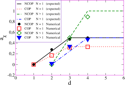
Figure 4: Exponent $a_{\chi}$ in different coarsening systems with scalar and vector order parameter, non-conserved and conserved order parameter Bray94 . The continuous lines represent Eq. (50), while the dots are the values from simulationspreprint ; generic .

VI.2.2 Roughening of interfaces

Apart from the few exact solutions mentioned above there is not a general derivation of Eq. (50) which, at this stage remains a phenomenological formula. For the case of a scalar order parameter, an argument has been proposed generic ; henkel04 explaining the dependence of $a_{\chi}$ on $d$ in terms of the roughening properties of the interfaces. It is based on two simple physical ingredients: a) the aging response is given by the density of defects $\rho(t)$ times the response of a single defect Corberi2001 $\chi_{ag}(t,s)=\rho(t)\chi_{ag}^{s}(t,s)$ and b) each defect responds to the perturbation by optimizing its position with respect to the external field in a quasi-equilibrium way. In $d=1$ this occurs via a displacement of the defect Corberi2001 . In higher dimensions, since defects are spatially extended, the response is produced by a deformation of the defect shape.

We develop the argument for a 2-d system, the extension to arbitrary $d$ being straightforward. A defect is a sharp interface separating two domains of opposite magnetization. In order to analyze $\chi_{ag}^{s}(t,s)$ we consider configurations with a single defect as depicted in Fig. 5. The corresponding integrated response function reads Corberi2001 $\chi_{ag}^{s}(t,s)=1/(h^{2}{\cal L}^{d-1})\int d{\text{x}}d{\text{y}}\,\overline{\langle\phi({\text{x}},{\text{y}})\rangle h({\text{x}},{\text{y}})}$, where $\phi({\text{x}},{\text{y}})$ is the order parameter field which saturates to $\pm 1$ in the bulk of domains, and ${\text{x}},{\text{y}}$ are space coordinates. $h({\text{x}},{\text{y}})$ is the external random field with expectations (41,42), and ${\cal L}$ is the linear system size. The overbar and angular brackets denote averages over the random field and thermal histories, respectively. With an interface of shape $z_{s}({\text{y}})$ at time $s$ (Fig. 5), we can write $\chi_{ag}^{s}(t,s)=-1/(h^{2}{\cal L}^{d-1})\overline{\int_{\{z\}}E_{h}\,P_{h}(\{z({\text{y}})\},t)}$, where $P_{h}(\{z({\text{y}})\},t)$ is the probability that an interface profile $\{z({\text{y}})\}$ occurs at time $t$ and $E_{h}=-\int_{0}^{\cal L}d{\text{y}}\int_{z_{s}({\text{y}})}^{z({\text{y}})}d{\text{x}}h({\text{x}},{\text{y}})\mbox{sign}[z({\text{y}})-z_{s}({\text{y}})]$ is the magnetic energy. We now introduce assumption b) making the ansatz for the correction to the unperturbed probability $P_{0}(\{z({\text{y}})\},t)$ in the form of a Boltzmann factor $P_{h}(\{z({\text{y}})\},t)=P_{0}(\{z({\text{y}})\},t)\exp(-E_{h}/T)\simeq P_{0}(\{z({\text{y}})\},t)[1-E_{h}/T]$. Then $\chi_{ag}^{s}(t,s)=-1/(h^{2}{\cal L}^{d-1})\overline{\int_{\{z\}}E_{h}(1-E_{h}/T)P_{0}(\{z({\text{y}})\},t)}$. Taking into account that the term linear in $E_{h}$ vanishes by symmetry and neglecting $z_{s}({\text{y}})$ with respect to $z({\text{y}})$ for $t\gg s$, we eventually find $T\chi_{ag}^{s}(t,s)={\cal L}^{1-d}\int_{\{z\}}\int_{0}^{\cal L}d{\text{y}}|z({\text{y}})|P_{0}(\{z({\text{y}})\},t)$. This defines a length which scales as the roughness of the interface given by $W(t)=[{\cal L}^{1-d}\int_{\{z\}}\int d{\text{y}}z({\text{y}})^{2}P_{0}(\{z({\text{y}})\},t)]^{1/2}$. The behavior of $W(t)$ in the coarsening process can be inferred from an argument due to Villain Abraham89 . In the case $d\leq 3$, when interfaces are rough Rough , for NCOP one has $W(t)\sim t^{(3-d)/4}$, while for COP $W(t)\sim t^{(3-d)/6}$, with logarithmic corrections in both cases for $d=3$. For $d>3$ interfaces are flat and $W(t)\simeq const.$ Finally, multiplying $\chi_{ag}^{s}$ by $\rho(t)\sim L(t)^{-1}$ Eq. (50) is recovered note2 and $d_{U}$ is identified with the roughening dimensionality $d_{R}=3$.

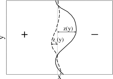
Figure 5: Configurations with a single interface at time $s$ (dashed line) and at time $t$ (continuous line).

VI.3 Statics from dynamics

We may now check if, and how, the connection between statics and dynamics discussed in Sec. V is realized in phase ordering systems. In the following we shall consider $d\geq d_{L}$.

In order to search for $S(C)$ in the case of phase ordering, let us set $\vec{r}=0$ in Eq. (38) and let us eliminate $t/s$ between $\widehat{\chi}_{ag}$ and $C_{ag}$ obtaining

$$\chi_{ag}(t,s)\sim s^{-a_{\chi}}\widetilde{\chi}_{ag}(C_{ag}).$$ (51)

Then, from Eqs.  (46,44,51) one can write the general relation

$$\chi(t,s)=\frac{1}{T}\left[C_{st}(\tau=0)-C_{st}(\tau)\right]+s^{-a_{\chi}}\widetilde{\chi}_{ag}(C_{ag}).$$ (52)

Using the identity $\left[C_{st}(\tau=0)-C_{st}(\tau)\right]=\left[C_{st}(\tau=0)+M^{2}-C_{st}(\tau)-M^{2}\right]$ and considering that, as shown schematically in Fig. 6, in the time interval where $C_{st}(\tau)\neq 0$, i.e. for short times, one can replace $C_{ag}(t/s)$ with $M^{2}$ or equivalently $C_{st}(\tau)+M^{2}=C(t,s)$, the above equation can be rewritten as

$$\chi(t,s)=\widetilde{\chi}_{st}(C)+s^{-a_{\chi}}\widetilde{\chi}_{ag}(C_{ag})$$ (53)

where the function $\widetilde{\chi}_{st}(C)$ is defined by

$$T\widetilde{\chi}_{st}(C)=\left\{\begin{array}[]{ll}\left[C(t,t)-C(t,s)\right]\qquad$for$\qquad M^{2}\leq C\leq C(t,t)\\ \left[C(t,t)-M^{2}\right]\qquad$for$\qquad C<M^{2}.\end{array}\right.$$ (54)

Therefore, from Eq. (53) we have that for phase ordering systems the fluctuation dissipation relation exists if $a_{\chi}>0$ (i.e. for $d>d_{L}$) and it is given by

$$S(C)=\widetilde{\chi}_{st}(C).$$ (55)

Computing the derivative in the left hand side of Eq. (29) and using Eqs. (55) and (54), for $d>d_{L}$ we find

$$\left.-T\frac{d^{2}S(C)}{dC^{2}}\right|_{C=q}=\delta(q-M^{2}).$$ (56)

Coming to statics, in replica symmetric low temperature states, as for instance in ferromagnetic systems, the overlap function is always trivial and, as anticipated in Sec. V, one has

$$P(q)=\frac{1}{2}\left[\delta(q-M^{2})+\delta(q+M^{2})\right],$$ (57)

with

$$\widetilde{P}(q)=\widehat{P}(q)=\delta(q-M^{2}).$$ (58)

as shown in Fig. 1 (I) (we recall that $q_{EA}=M^{2}$ in this case). From Eqs. (58,56), therefore, Eq. (29) is satisfied, and the connection between statics and dynamics holds.

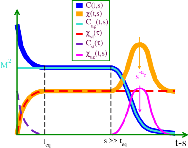
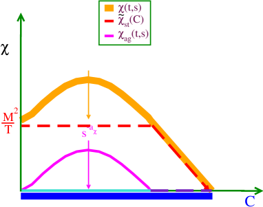
Figure 6: Schematic plot of the behavior of the two time functions in the coarsening stage as $t-s$ is varied keeping $s$ fixed (upper figure), and of the resulting fluctuation dissipation plot (lower figure). The stationary parts $C_{st}$, $\chi_{st}$, as discussed in Secs. VI.1,VI.2, saturate to their final value on times $\tau\simeq t_{eq}$; the aging parts $C_{ag}$, $\chi_{ag}$, according to the scaling forms (38,47) remain constant up to times $t-s\simeq s$. The magnitude of $\chi_{ag}$ is proportional to $s^{-a_{\chi}}$, and decreases as $s$ is increased (shown by an arrow in Figure).

For $a_{\chi}=0$ a little more care is needed. Equation (53) yields $\chi(t,s)=\widetilde{\chi}_{st}(C)+\widetilde{\chi}_{ag}(C_{ag})$. Recalling that $a_{\chi}=0$ occurs at $d=d_{L}$, which coincides with the lower critical dimensionality, in order to have a phase ordering process a quench to $T=0$ is required. This, in turn, implies $C_{st}(t,s)=0$ and $C_{ag}(t,s)=C(t,s)$. Therefore, using Eq. (54) we have

$$S(C)=\chi_{eq}^{*}+\widetilde{\chi}_{ag}(C)$$ (59)

where $\chi_{eq}^{*}=\lim_{T\rightarrow 0}[C(0)-M^{2}]/T$ is the $T=0$ equilibrium susceptibility, which vanishes for hard spins while is different from zero for soft spins. Therefore the FDR exists also in this case. However, while for $a_{\chi}>0$ $\chi_{ag}$ eventually disappears and Eq. (45) holds, this is no longer true for $d=d_{L}$. Here $a_{\chi}=0$ and, consequently, as can be seen from Eq. (59) $\chi_{ag}$ gives a contribution to the response which persists also in the asymptotic time region. Then Eq. (45), and hence condition (2) above Eq. (29 are not fulfilled. Being one of the hypothesis leading to Eq. (29) violated, the connection between statics and dynamics could not hold. Actually, in all the model explicitly considered in the literature Corberi2001 ; preprint ; generic it turns out that at $d=d_{L}$ $S(C)$ is a non-trivial dynamical function unrelated to $\widetilde{P}(q)$. For the sake of definiteness, let us discuss the case of the Ising model with $d=1$ Godreche ; Lippiello2000 . In order to make compatible the two requirements of having an ordered equilibrium state and a well defined linear response function, instead of taking the $T\rightarrow 0$ limit it is necessary to take the limit of an infinite ferromagnetic coupling Lippiello2000 . Then, $P(q)$ and $\widetilde{P}(q)$ are given by Eqs. (57) and (58) with $M^{2}=1$ at all temperatures. On the other hand, for any $T$ one also have Lippiello2000 (see Fig. 7)

$$T\widetilde{\chi}_{ag}(C)=\frac{\sqrt{2}}{\pi}\arctan\left[\sqrt{2}\cot\left(\frac{\pi}{2}C\right)\right].$$ (60)

This gives

$$\left.-T\frac{d^{2}S(C)}{dC^{2}}\right|_{C=q}=\frac{\pi\cos(\pi q/2)\sin(\pi q/2)}{[2-\sin(\pi q/2)]^{2}}.$$ (61)

Hence, it is clear that Eq. (29) is not verified. The reason is that the second of the above conditions required for establishing the connection is not satisfied. In fact, from Eqs. (53) and (60), keeping in mind that the limits $t\rightarrow\infty$ and $C\rightarrow 0$ are equivalent, we have

$$\lim_{t\rightarrow\infty}T\chi(t,s)=1/\sqrt{2}$$ (62)

which is responsible of the violation of condition (2) above Eq. (29), since in this case $\chi_{eq}=0$. Interestingly, a similar behavior is observed prlparma also for the Ising model on graphs with $T_{c}=0$, which, in a sense, can be regarded as being at $d_{L}$.

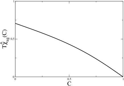
Figure 7: Fluctuation dissipation plot for the 1d-Ising model.

VI.3.1 Role of quenched disorder at $d=d_{L}$

The behavior of the exponent $a_{\chi}$, and its vanishing at $d_{L}=1$ can be qualitatively interpreted in terms of the behavior of the response $\chi^{s}_{ag}(t,s)$ associated to a single interface. In $d=1$ it can be shown exactly Corberi2001 that $\chi^{s}_{ag}(t,s)\propto(t-s)^{1/2}$. Therefore, when computing the total response through $\chi_{ag}(t,s)\simeq\rho(t)\chi^{s}(t,s)$ the loss of interfaces described by $\rho(t)$ is exactly balanced by the increase of $\chi^{s}(t,s)$, which leads to a finite $\lim_{t\to\infty}\chi_{ag}(t,s)$. This in turn is responsible for the breakdown of the condition (2) above Eq. (29). For $d>d_{L}$, instead, the growth of $\chi^{s}(t,s)$ is not sufficient Corberi2001 to balance the decrease of $\rho(t)$. This happens because, while in $d=1$ interfaces are Brownian walkers, free to move in order to maximize the response, for $d>1$ this issue is contrasted by surface tension, restoring the validity of condition (2). In this Section how a similar effect, namely a reduction of the response of interfaces, can be produced, also in $d=1$, by the presence of quenched disorder.

Let us consider the case of the $d=1$ random field Ising model (RFIM). In the presence of a quenched random field, domain walls perform random walks in a random potential of the Sinai type and the average domain size $L(t)$ behaves as the root mean square displacement of the random walkerFisher01 . The typical potential barrier encountered by a walker after traveling a distance $l$ is order of $\sqrt{l\sigma_{h}}$ where $\sigma_{h}$ is the variance of the random field. Hence, there exists a characteristic length $L_{g}=T^{2}/\sigma_{h}$ representing the distance over which potential barriers are of the order of magnitude of thermal energy. For displacements much less than $L_{g}$ diffusion takes place in a flat landscape like in the pure system and $L(t)\sim t^{1/2}$. For displacements much greater than $L_{g}$, instead, one finds the SinaiSinai82 diffusion law $L(t)\sim(\ln t)^{2}$. The response function obeysCorberi4 the scaling relation (Fig. 8)

$$T\chi_{\text{ag}}(t,s,L_{g})=\widetilde{\chi}\left(\frac{L(t)}{L(s)},z\right)$$ (63)

where $z=L(s)/L_{g}$. For $z=0$ the form of the response function for the pure system is recovered. With $z>0$ there is a crossover. The pure case behavior holds for $L(t)-L(s)\ll L_{g}$, while for $L(t)-L(s)>L_{g}$ the response levels off and then decreases. This is clearly displayed also in the plot (Fig. 9) against the autocorrelation function. Looking at the effective response of a single interface $\chi^{s}(t,s)$ one finds $\chi^{s}(t,s,L_{g})=L(s)\widetilde{\chi}^{s}\left(\frac{L(t)}{L(s)},z\right)$ with the scaling function displaying the behavior

$$\widetilde{\chi}^{s}(x,z)\sim\left\{\begin{array}[]{ll}x\widetilde{\chi}(x,z=0)&\mbox{, for $x-1\ll 1/z$}\\ \sqrt{x}&\mbox{, for $x-1\gg 1/z$.}\end{array}\right.$$ (64)

From this follows ${\chi}^{s}(t,s)\geq\rho_{I}^{-1}(t)$ in the preasymptotic regime and ${\chi}^{s}(t,s)\sim\rho_{I}^{-1/2}(t)$ in the asymptotic regime, which account for the crossover of the response function in Figs. 8,9 in terms of the balance between the rate of growth of the single interface response and the rate of loss of interfaces. Hence, for $z>0$ eventually $\widetilde{\chi}(x,z)$ vanishes and in the limit $z\rightarrow\infty$ one expects $\chi_{\text{ag}}(x,z=\infty)\equiv 0$. Therefore, for any finite quenched random field the validity of Eq. (29) is restored.

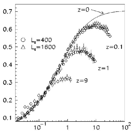
Figure 8: The ZFC $\chi_{ag}(t,s)$ is plotted versus the the ratio $[L(t)-L(s)]/L(s)$, for $L_{g}=400,1600$, and $z=0.1,9$. The solid line is the exact result for $z\to 0$.

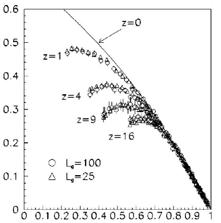
Figure 9: The ZFC $\chi_{ag}(t,s)$ is plotted versus the autocorrelation function $C(t,s)$, for $L_{g}=25,100$, and $z=1,4,9,16$. The solid line is the exact result for $z\to 0$.

VI.3.2 Failure by stochastic instability

An interesting example Fusco , where statics cannot be reconstructed from dynamics because the third requirement of stochastic stability is not satisfied, comes from the spherical model. More precisely, one must consider in parallel the original version of the spherical model (SM) of Berlin and Kac Berlin and the mean spherical model (MSM) introduced by Lewis and Wannier Lewis , with the spherical constraint treated in the mean. These two models are equivalent above but not below $T_{C}$ Kac . The low temperature states are quite different, with a bimodal order parameter probability distribution in the SM case and a Gaussian distribution centered in the origin in the MSM case. The corresponding overlap functions are also very different Fusco . Considering, for simplicity, $T=0$ one has

$$P(q)=\left\{\begin{array}[]{ll}\frac{1}{2}\left[\delta(q-M^{2})+\delta(q+M^{2})\right]\qquad$for SM$\\ \frac{1}{\pi M^{2}}K_{0}(|q|/M^{2})\qquad$for MSM$\end{array}\right.$$ (65)

where $K_{0}$ is a Bessel function of imaginary argument (Fig.10).

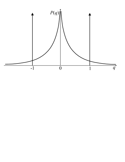
Figure 10: Overlap distribution for mean spherical model with $M^{2}=1$. The arrows represent the $\delta$ functions of the overlap distribution for the spherical model.

However, after switching of an external field, one finds for both models $\widetilde{P}(q)=\delta(q-M^{2})$. This means that stochastic stability holds for SM but not for MSM.

On the other hand, the relaxation properties are the same in the two models, both above and below $T_{C}$ if the thermodynamic limit is taken before the $t\rightarrow\infty$ limit Fusco . Then, the linear response function is the same for both models and obeys Eq. (53) with $a_{\chi}$ given by Eq. (50), where $\delta$, $d_{L}$ and $d_{U}$ are the same as for the large $N$ model (Table I). Hence, we have that although Eq. (29) is satisfied for both models, nonetheless statics and dynamics are connected only in the SM case, where $\widetilde{P}(q)=\widehat{P}(q)$. Instead, this is not possible in the MSM case where $\widetilde{P}(q)\neq\widehat{P}(q)$.

VII Conclusions

In this Article we have reviewed some recent progresses in the field of non-equilibrium linear response theory. A first accomplishment is the derivation of a generalization of the FDT for Markov processes which allows the computation of the response function in terms of correlation functions of the unperturbed system. This represents a great simplification particularly in numerical calculations, which are usually computationally very demanding: The generalization of the FDT allows a sensible speed and precise numerical determination of the response function can be achieved. This quantity has been deeply investigated particularly in the field of slowly relaxing systems, because its relation with the autocorrelation function represents a bridge between statics and dynamics.

Phase-ordering systems can be regarded as the simplest instance of aging systems, where the behavior of the response function can be more easily investigated. In this context, a partial understanding has been achieved by matching the results of numerical simulations with the outcomes of solvable models and approximate theories, showing that the scaling properties of the response function are non-trivial. In particular, Eq. (47) is obeyed with $a_{\chi}$ depending on dimensionality through the phenomenological formula (50), which is found to be consistent with all the cases considered in the literature and, for the scalar case is supported by an argument based on the roughness properties of the interfaces. The dependence of $a_{\chi}$ on dimensionality is such that it vanishes at the lower critical dimension. This implies an asymptotic finite contribution of the aging part of the response function which invalidates the connection between statics and dynamics. Phase ordering therefore offers examples where a replica symmetric low temperature state is compatible with a non trivial FDR which, therefore, cannot be used to infer the properties of the equilibrium state.

This whole phenomenology is not adequately captured by the existing approaches to phase-ordering. Theories based on the GAF method, originally introduced by Otha, Jasnow and Kawasaki ojk , provide the phenomenological formula (50) but with a wrong value $d_{U}=2$ Berthier99 ; Corberi2001 . This discrepancy is not removed using a perturbative expansion Mazenko2004 developed to improve over the GAF approximation. Next to these theories, it is of much interest the approach by Henkel et al. Henkel2001 , based on the conjecture that the response function transforms covariantly under the group of local scale transformations. This ansatz, however, fixes the form of the scaling function in Eq. (47) but not the exponent $a_{\chi}$ which remains insofar an undetermined quantity. A first principle theory for the complete description of the behavior of the linear response function in phase-ordering systems may represent a pre-requisite for understanding the behavior of more complex systems, like glasses and spin glasses. However, despite some progresses of a specific character, such a theory is presently still lacking.

References

- (1) R. Kubo, M. Toda and N. Hashitsume, Statistical Physics, vol.2 (Springer, Berlin, 1985).
- (2) P.C. Hohenberg and B.I. Shraiman, Physica D 37, 109 (1989).
- (3) L.F. Cugliandolo and J. Kurchan, Phys.Rev.Lett. 71, 173 (1993); Philos.Mag. 71, 501 (1995); J.Phys. A 27, 5749 (1994).
- (4) L.F. Cugliandolo, J. Kurchan, and L. Peliti Phys. Rev. E 55, 3898 (1997).
- (5) L. Berthier, J.-L. Barrat and J. Kurchan, Phys. Rev. E 61, 5464 (2000).
- (6) S. Fielding and P. Sollich, Phys. Rev. Lett. 88, 050603 (2002); cond-mat/0209645.
- (7) L. Cugliandolo, J. Kurchan and G. Parisi, J.Phys.I France 4, 1641 (1994).
- (8) E. Lippiello, F. Corberi, and M. Zannetti, Phys.Rev.E 71, 036104 (2005).
- (9) S.Franz, M.Mézard, G.Parisi and L.Peliti, Phys.Rev.Lett. 81, 1758 (1998); J.Stat.Phys. 97, 459 (1999).
- (10) G.Parisi, F.Ricci-Tersenghi and J.J.Ruiz-Lorenzo, Eur.Phys.J.B 11, 317 (1999).
- (11) For a review see A.J.Bray, Adv.Phys. 43, 357 (1994).
- (12) C.Chatelain, J.Phys. A 36, 10739 (2003).
- (13) A. Crisanti and F. Ritort, J.Phys. A 36, R181 (2003).
- (14) N. Andrenacci, F. Corberi, and E. Lippiello Phys. Rev. E 73, 046124 (2006).
- (15) F. Ricci-Tersenghi, Phys.Rev.E 68, 065104(R) (2003).
- (16) G. Diezeman, cond-mat/0309105.
- (17) F.Guerra, Int.J.Mod.Phys. B 10, 1675 (1997).
- (18) M.Mézard, G.Parisi and M.A.Virasoro, Spin Glass Theory and Beyond. World Scientific (Singapore 1987).
- (19) G.Parisi, Phys. Rev. Lett. 79, 3660 (1997).
- (20) J.L.Barrat and W.Kob, Europhys. Lett. 46, 637 (1999).
- (21) For a different perspective to compare these two classes of systems see also: C. Chamon, L. Cugliandolo and H. Yoshino, J. Stat. Mech., P01006 (2006).
- (22) For a recent review see L.F.Cugliandolo Dynamics of glassy systems Lecture notes, Les Houches, July 2002, cond-mat/0210312.
- (23) R.G.Palmer, Adv.Phys. 31, 669 (1982).
- (24) J.Kurchan and L.Laloux, J.Phys.A: Math.Gen. 29, 1929 (1996).
- (25) C.M.Newman and D.L.Stein, J.Stat.Phys. 94, 709 (1999).
- (26) H.Furukawa, J.Stat.Soc.Jpn. 58, 216 (1989); Phys.Rev. B 40, 2341 (1989).
- (27) See for instance J.P.Bouchaud, L.F.Cugliandolo, J.Kurchan and M.Mézard in Spin Glasses and Random Fields edited by A.P.Young (World Scientific, Singapore, 1997).
- (28) A.Barrat, Phys.Rev.E 57, 3629 (1998).
- (29) E.Lippiello and M.Zannetti, Phys.Rev. E 61, 3369 (2000).
- (30) C.Godrèche and J.M.Luck, J.Phys.A: Math.Gen. 33, 1151 (2000).
- (31) F.Corberi, E.Lippiello and M.Zannetti, Phys.Rev. E 65, 046136 (2002).
- (32) L.Berthier, J.L.Barrat and J.Kurchan, Eur.Phys.J.B 11, 635 (1999).
- (33) F.Corberi, E.Lippiello and M.Zannetti, Eur.Phys.J.B 24, 359 (2001).
- (34) F.Corberi, E.Lippiello and M.Zannetti, Phys.Rev.Lett. 90, 099601 (2003).
- (35) F.Corberi, E.Lippiello and M.Zannetti, Phys.Rev. E 68, 046131 (2003).
- (36) F.Corberi, E.Lippiello, M.Zannetti and C.Castellano, Phys. Rev. E 70, 017103 (2004).
- (37) F. Corberi, E. Lippiello, and M. Zannetti, Phys. Rev. E 74, 041106 (2006).
- (38) M. Henkel, M. Paessens and M. Pleimling, Phys. Rev. E 69, 056109 (2004).
- (39) The argument is quoted in D. B. Abraham and P. J. Upton, Phys. Rev. B 39, 736 (1989).
- (40) A.-L. Barabási and H. E. Stanley, Fractal Concepts in Surface Growth, (Cambridge University Press, Cambridge, 1995).
- (41) This argument holds also for Ising spins. Only for differences arise when the Ising model undergoes a roughening transition at the temperature between a low phase with flat (faceted) domain walls and a rough high phase [see T. Emig and T. Nattermann, Eur. Phys. J. B 8, 525 (1999).] Hence we expect logarithmic corrections in Eq. (50) only for , and a pure algebraic decay for . A numerical test of this prediction would be of great interest, but very demanding from the computational point of view.
- (42) R.Burioni, D.Cassi, F.Corberi, and A.Vezzani Phys. Rev. Lett. 96, 235701 (2006); Phys. Rev. E 75, 011113 (2007).
- (43) D.S.Fisher, P.Le Doussal and C.Monthus, cond-mat/0012290.
- (44) Y.G.Sinai, Theor.Prob.Appl. 27, 256 (1982).
- (45) F.Corberi, A.de Candia, E.Lippiello and M.Zannetti, Phys. Rev. E 65, 046114 (2002).
- (46) N.Fusco and M.Zannetti, Phys.Rev.E 66, 066113 (2002).
- (47) T.H.Berlin and M.Kac, Phys.Rev. 86, 821 (1952).
- (48) H.W.Lewis and G.H.Wannier, Phys.Rev. 88, 682 (1952); 90, 1131E (1953).
- (49) M.Kac and C.J.Thompson, J.Math.Phys. 18, 1650 (1977).
- (50) T. Otha, D. Jasnow and K. Kawasaki, Phys. Rev. Lett. 49, 1223 (1982).
- (51) G. Mazenko, Phys. Rev. E 69, 016114 (2004).
- (52) M. Henkel, M. Pleimling, C. Godrèche and J.M. Luck, Phys. Rev. Lett. 87, 265701 (2001); M. Henkel, Nucl. Phys. B 641, 405 (2002).