Electroweak Hard Photon Bremsstrahlung in Electron-Nucleon Scattering

Abstract

One way to treat the infrared divergences of the electroweak Next-to-Leading-Order (NLO) differential cross sections to parity-violating (PV) electron-proton scattering is by adding soft-photon emission contribution. Although more physical, the results are left with a logarithmic dependence on the photon detector acceptance, which can only be eliminated by considering Hard Photon Bremsstrahlung (HPB) contribution. Here we present a treatment of HPB for PV electron-proton scattering. HPB differential cross sections for electron-proton scattering have been computed using the experimental values of nucleon form factors. The final results are expressed through kinematic parameters, making it possible to apply the computed PV HPB differential cross sections for the analysis of data of a range of current and proposed experiments.

I Introduction

Electroweak properties of the nucleon can be studied by parity-violating electron-nucleon scattering at low to medium energies Bec89 . Such experiments can measure the asymmetry factor coming from the difference between cross sections of left- and right-handed electrons. This asymmetry between left- and right-handed particles, as a result of a parity-violating interference between the weak and electromagnetic forces, is clearly predicted in the Standard Model of Particle Physics.

Extracting the physics of interest from the measured asymmetry requires evaluating NLO contribution to electroweak scattering at very high precision. The method for evaluation of the electron-nucleon up to NLO differential cross sections most commonly found in the literature is to follow the Feynman rules for the particles of the Standard Model. The dominant contribution normally comes from the leading order (LO) correction in perturbation theory. Some of the electroweak NLO contributions to intermediate energy, parity non-conserving semi-leptonic neutral current interactions have been addressed previously in Mus89 ; MH90 ; MH91 ; Mus94 . Ref. Zhu00 also estimated effects due to an intrinsic weak interaction in the nucleon (e. g. the anapole moment) in chiral perturbation theory, and found the anapole moment contributions insignificant, only slightly enhancing the axial vector NLO contribution.

Later work in BAB2002 took the advantage of the modern computational opportunities and improved the techniques for one-quark NLO computation by retaining analytical momentum-dependent expressions, and providing the numerical evaluations of 446 one-loop diagrams. It also included calculation of the soft photon emission contribution. However, in BAB2002 , even after removing infra-red (IR) divergences through soft-photon emission corrections, calculated one-quark NLO contribution show a logarithmic dependence on the detector’s photon acceptance parameter $\Delta E$.

The article presented here demonstrates that elimination of this dependence can be achieved by adding the Hard-Photon Bremsstrahlung (HPB) differential cross section. We express general electroweak couplings by inserting appropriate form factors into vertices and construct HPB differential cross sections as a function of Mandelstam invariants. For each set of experimental constraints, integration over the emitted photon phase space can be performed numerically. Analytical results of this article can be used for several recent PV experiments SAMPLE ; SAMPLEIII ; HAPPEX ; G0 ; A4 ; Qweak .

The article provides a detailed description of both hard- and soft-photon emission treatment of infrared divergences the PV electroweak interference and pure weak contributions to the total differential cross section. As an example, we choose to consider electron-proton scattering, as one of the most relevant cases from a physics perspective. However, the same technique of treating infrared (IR) divergences can be expanded to neutron or any other baryon target if same effective structure of the coupling is used.

II Soft-Photon Bremsstrahlung

If the structure of the nucleon is investigated using weak, neutral current probe G0 ; SAMPLE ; HAPPEX , it is necessary to enhance the weak contribution in electron-nucleon scattering by exploiting the parity-violating nature of the weak interactions and constructing the following quantity (asymmetry):

$$A=\frac{d\sigma_{R}^{tot}-d\sigma_{L}^{tot}}{d\sigma_{R}^{tot}+d\sigma_{L}^{tot}}\cong\frac{Re\left(M_{LO}^{\gamma}M_{LO+NLO}^{Z}\right)_{R}-Re\left(M_{LO}^{\gamma}M_{LO+NLO}^{Z}\right)_{L}}{\left|M_{LO}^{\gamma}\right|_{R(L)}^{2}} =$$

$$=A_{LO}+\frac{Re\left(M_{LO}^{\gamma}M_{NLO}^{Z}\right)_{R}-Re\left(M_{LO}^{\gamma}M_{NLO}^{Z}\right)_{L}}{\left|M_{LO}^{\gamma}\right|_{R(L)}^{2}}.$$

Here, $A_{LO}$ is a leading order asymmetry measured in the parts per million (ppm) and second term of Eq.(LABEL:eq:pv1) is a parity-violating NLO contribution to the asymmetry.

Finally, if the axial-vector ($C_{1}$) or vector-axial ($C_{2}$) form factors of the parity violating amplitude are studied Qweak , which can be taken from PV Hamiltonian

$$H^{PV}=\frac{G_{F}}{\sqrt{2}}\left[C_{1}\left(\overline{u}_{e}\gamma^{\mu}\gamma^{5}u_{e}\right)\left(\overline{u}_{N}\gamma^{\mu}u_{N}\right)+C_{2}\left(\overline{u}_{e}\gamma^{\mu}u_{e}\right)\left(\overline{u}_{N}\gamma^{\mu}\gamma^{5}u_{N}\right)\right],$$ (2)

with perturbative expansion resulting in

$$C_{1,2}=C_{1,2}^{LO}+C_{1,2}^{NLO}+O\left(\alpha^{3}\right).$$ (3)

All of the above NLO contributions to the either asymmetry (Eq.(LABEL:eq:pv1)) or PV form-factor (Eq.(3)) in general can be infra-red divergent HooftVelt72 , and can be treated by the soft and hard-photon emission contribution shown on Fig. (1).

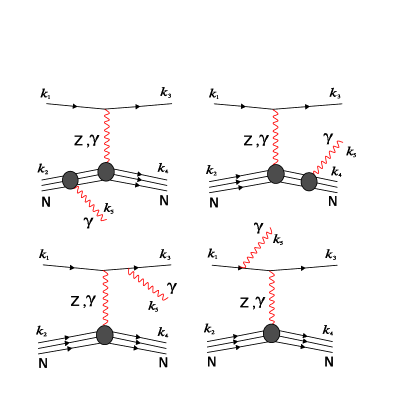
Figure 1: Hard Photon Bremsstrahlung diagrams in electron-proton scattering.

The differential cross section associated with bremsstrahlung emission in electron-nucleon scattering can be described by the following formula,

$$d\sigma_{B}\propto\left|M_{B}^{\gamma}+M_{B}^{Z}\right|^{2}=\left|M_{B}^{\gamma}\right|^{2}+2Re\left(M_{B}^{\gamma}M_{B}^{Z}\right)+\left|M_{B}^{Z}\right|^{2}.$$ (4)

The first term of Eq.(4) is responsible for the cancellation of IR divergences if a parity conserving electromagnetic probe is used. The second term, when used in the asymmetry

$$A_{B}\propto\frac{Re\left(M_{B}^{\gamma}M_{B}^{Z}\right)_{R}-Re\left(M_{B}^{\gamma}M_{B}^{Z}\right)_{L}}{\left|M_{LO}^{\gamma}\right|_{R(L)}^{2}},$$ (5)

is responsible for canceling IR divergences in Eq.(LABEL:eq:pv1). Finally, IR divergences in the NLO form-factors (Eq.(3)) are indirectly treated by the third term of Eq.(4), and will be discussed later in this article.

Generally, bremsstrahlung diagrams can be described as $2\rightarrow 3$ processes in which integration over emitted photon’s phase space should be performed. If the momentum of the emitted photon is small enough to be neglected in the numerator algebra, we can present the bremsstrahlung cross section as a soft photon factor multiplied by the tree level differential cross section of $2\rightarrow 2$ process.

Let us consider an example. The scattering amplitude for the first diagram of Fig.(1), for the neutral current reaction, has the following structure:

$$M_{B}^{Z} = \left\langle\overline{u}(m_{e},k_{3})\right|\Gamma_{Z-e}^{\nu}\left|u(m_{e},k_{1})\right\rangle\times$$

$$\quad\left\langle\overline{u}(m_{N},k_{4})\right|\Gamma_{Z-N}^{\mu}(q)\frac{\not k_{2}-\not k_{5}+m_{N}}{(k_{2}-k_{5})^{2}-m_{N}^{2}}\Gamma_{\gamma-N}^{\alpha}(k_{5})\left|u(m_{N},k_{2})\right\rangle\times$$

$$\quad\frac{g_{\mu\nu}}{(k_{4}-k_{2}+k_{5})^{2}-m_{Z}^{2}}\varepsilon_{\alpha}^{*}(k_{5}),$$

where the photon polarization vector enters as $\varepsilon_{\alpha}(k_{5})$; $\Gamma_{Z-e}^{\nu},\,\Gamma_{Z-N}^{\mu}$ and $\Gamma_{\gamma-N}^{\alpha}$ are the couplings of electron with Z boson, nucleon with Z boson, and photon with nucleon, respectively, defined as

$$\Gamma_{Z-e}^{\nu} = ie\left[-\frac{1-2s_{W}^{2}}{2c_{W}\,s_{W}}\gamma^{\nu}\varpi_{-}+\frac{s_{W}}{c_{W}}\gamma^{\nu}\varpi_{+}\right],$$

$$\Gamma_{Z-N}^{\mu}\,(q) = ie\left[f_{1}(q)\gamma^{\mu}+\frac{i}{2m_{N}}\sigma^{\mu\rho}q_{\rho}\,f_{2}(q)+g_{1}(q)\gamma^{\mu}\gamma_{5}\right],$$ (6)

$$\Gamma_{\gamma-N}^{\alpha}\,(q) = ie\left[F_{1}(q)\gamma^{\alpha}+\frac{i}{2m_{N}}\sigma^{\alpha\rho}(q)_{\rho}F_{2}(q)\right].$$

Here $q$ corresponds to the momentum transferred to the nucleon from the vector boson. The shortened notation of $s_{W}$ and $c_{W}$ refers to $\sin\theta_{W}$ and $\cos\theta_{W}$, the Weinberg mixing angle. For the form factors $f_{1,2}(q),$ $F_{1,2}(q),$ and $g_{1}(q)$ we have used

$$f_{1,2}(q) = \frac{1}{4s_{W}\,c_{W}}\left(F_{1,2}^{V\left(N\right)}-4s_{W}^{2}F_{1,2}\right)G_{N}\left(q\right),$$

$$F_{1,2}\left(q\right) = F_{1,2}(0)G_{N}\left(q\right),$$

$$F_{1,2}^{V\left(n\right)}\left(0\right) = F_{1,2}^{n}\left(0\right)-F_{1,2}^{p}\left(0\right),\,\,\,\,F_{1,2}^{V\left(p\right)}\left(0\right)=F_{1,2}^{p}\left(0\right)-F_{1,2}^{n}\left(0\right),$$

$$g_{1}(q) = -\frac{g_{A}(0)}{4s_{W}\,c_{W}}G_{N}\left(q\right),$$

with $F_{1,2}\left(0\right)$ and $g_{A}\left(0\right)$ defined as the nucleon’s Dirac, Pauli, and axial form factors at zero momentum transfer and corresponds to the electric charge, anomalous magnetic moment, and axial charge, respectively. Here, we use the universal formfactor of monopole or dipole type $G_{N}\left(q\right)=\left(\frac{\Lambda^{2}}{\Lambda^{2}-q^{2}}\right)^{n}$ with $n=1,2$ and $\Lambda^{2}=0.83m_{N}^{2}.$

In the soft-photon emission limit the coupling between the emitted photon and the nucleon, $\Gamma_{\gamma-N}^{\alpha}(k_{5})$, is just equal to $ieQ\gamma^{\alpha}$, where charge $Q=1(0)$ for proton (neutron). The numerator of nucleon’s propagator $\not k_{2}-\not k_{5}+m_{N}$ can be replaced by $\not k_{2}+m_{N},$ and $(k_{2}-k_{5})^{2}-m_{N}^{2}$ can be easily simplified into $-2\left(k_{2}\cdot k_{5}\right)$. Using the Dirac equation for free spinors, we have

$$\frac{\not k_{2}+m_{N}}{-2\left(k_{2}\cdot k_{5}\right)}ieQ\gamma^{\alpha}\left|u(m_{N},k_{2})\right\rangle\varepsilon_{\alpha}(k_{5}) = -ieQ\frac{\not k_{2}\gamma^{\alpha}+\gamma^{\alpha}\not k_{2}}{2\left(k_{2}\cdot k_{5}\right)}\left|u(m_{N},k_{2})\right\rangle\varepsilon_{\alpha}^{*}(k_{5})$$

$$= -ieQ\frac{(k_{2}\cdot\varepsilon^{*}(k_{5}))}{(k_{2}\cdot k_{5})}\left|u(m_{N},k_{2})\right\rangle.$$

Now we can present the soft-photon amplitude in the following form:

$$M_{B}^{soft} = \left\langle\overline{u}(m_{e},k_{3})\right|\Gamma_{Z-e}^{\nu}\left|u(m_{e},k_{1})\right\rangle\left\langle\overline{u}(m_{N},k_{4})\right|\Gamma_{Z-N}^{\mu}(q)\left|u(m_{N},k_{2})\right\rangle\times$$

$$\frac{g_{\mu\nu}}{(k_{4}-k_{2}+k_{5})^{2}-m_{Z}^{2}}\left(-ieQ\frac{(k_{2}\cdot\varepsilon^{*}(k_{5}))}{(k_{2}\cdot k_{5})}\right)$$

$$= M_{LO}\left(-ieQ\frac{(k_{2}\cdot\varepsilon^{*}(k_{5}))}{(k_{2}\cdot k_{5})}\right)=M_{LO}\kappa(k_{2},k_{5}).$$

Here, $M_{LO}$ is a tree level amplitude of $2\rightarrow 2$ process. Eq.(LABEL:br1.4a) can be used for the other photon emission diagrams with a different factor $\kappa(k_{i},k_{5})=\pm ieQ_{i}\frac{(k_{i}\cdot\varepsilon^{*}(k_{5}))}{(k_{i}\cdot k_{5})}$. Now we can sum over all four graphs on Fig.(1) and square the total amplitude to get the following:

$$\left|M_{B}^{soft}\right|^{2}=\left|M_{LO}\right|^{2}e^{2}\left|\frac{(k_{1}\cdot\varepsilon^{*}(k_{5}))}{(k_{1}\cdot k_{5})}-Q\frac{(k_{2}\cdot\varepsilon^{*}(k_{5}))}{(k_{2}\cdot k_{5})}-\frac{(k_{3}\cdot\varepsilon^{*}(k_{5}))}{(k_{3}\cdot k_{5})}+Q\frac{(k_{4}\cdot\varepsilon^{*}(k_{5}))}{(k_{4}\cdot k_{5})}\right|^{2}.$$ (10)

The photon couples to a current which is conserved: $k^{\mu}M_{\mu}=0.$ This fact, and the summation over all photon polarizations gives us the possibility to replace $\sum_{\varepsilon}(k_{i})^{\mu}(k_{j})^{\nu}\varepsilon_{\mu}^{*}\varepsilon_{\nu}$ with $-g_{\mu\nu}(k_{i})^{\mu}(k_{j})^{\nu}=-(k_{i}\cdot k_{j})$. The last step is to integrate over the emitted photon phase space $d\Gamma_{k_{5}}=\frac{d^{3}k_{5}}{\left(2\pi^{3}\right)\,2k_{5}^{0}}$ and regularize the infrared divergence by assigning to the photon small rest mass $\lambda.$ This dependence on the rest mass of the photon will be canceled when added to IR divergent NLO contribution (see Eqs.(LABEL:eq:pv1, 5)). The resulting soft-photon emission differential cross section is expressed as

$$d\sigma_{soft} = d\sigma_{LO}^{2\rightarrow 2}\left(-\frac{\alpha^{2}}{2\pi^{2}}\right)\int_{\lambda\leq\left|k_{5}^{0}\right|\leq\Delta E}\frac{d^{3}k_{5}}{2\sqrt{k_{5}^{2}+\lambda^{2}}}\left(\begin{array}[]{c}\frac{k_{1}}{(k_{1}\cdot k_{5})}-Q\frac{k_{2}}{(k_{2}\cdot k_{5})}-\\ \\ \frac{k_{3}}{(k_{3}\cdot k_{5})}+Q\frac{k_{4}}{(k_{4}\cdot k_{5})}\end{array}\right)^{2}$$ (14)

$$= d\sigma_{LO}^{2\rightarrow 2}\,\left(-\frac{\alpha^{2}}{2\pi^{2}}\right)(2m_{e}^{2}\,I\left(k_{1},k_{1}\right)-(2m_{e}^{2}-t)\,I\left(k_{1},k_{3}\right)+2Q^{2}m_{N}^{2}\,I\left(k_{2},k_{2}\right)-$$

$$\ \ Q^{2}(2m_{N}^{2}-t)\,I\left(k_{2},k_{4}\right)-2Q\,(u-m_{e}^{2}-m_{N}^{2})\,I\left(k_{1},k_{4}\right)-2(s-m_{e}^{2}-m_{N}^{2})\,I\left(k_{1},k_{2}\right))$$

$$= d\sigma_{LO}^{2\rightarrow 2}\cdot\delta_{soft}.$$ (15)

Here $\Delta E$ is the maximum possible energy of emitted photon for which the soft-photon approximation is still valid. Numerical analysis leads to a typical constraint $\lambda<\Delta E\leq 10^{-3}E_{cms}$.

In Eq.(15), $I\left(k_{i},k_{j}\right)=\int_{\left|k_{5}\right|\leq\Delta E}\frac{d^{3}k_{5}}{2\sqrt{k_{5}^{2}+\lambda^{2}}}\frac{1}{(k_{i}\cdot k_{5})(k_{j}\cdot k_{5})}$ is the soft-photon emission integral evaluated earlier by HooftVelt72 , and equal to

$$I\left(k_{i},k_{j}\right)=\frac{2\pi\alpha_{ij}}{\alpha_{ij}^{2}m_{i}^{2}-m_{j}^{2}}\left[\begin{array}[]{c}\frac{1}{2}\ln\left(\frac{\alpha_{ij}^{2}m_{i}^{2}}{m_{j}^{2}}\right)\ln\left(\frac{4\Delta E^{2}}{\lambda^{2}}\right)+\frac{1}{4}\ln^{2}\left(\frac{E_{i}-\left|k\right|_{i}}{E_{i}+\left|k\right|_{i}}\right)-\frac{1}{4}\ln^{2}\left(\frac{E_{j}-\left|k\right|_{j}}{E_{j}+\left|k\right|_{j}}\right)+\\ \\ Li_{2}\left(1-\frac{\alpha_{ij}}{v_{ij}}\left(E_{i}+\left|k\right|_{i}\right)\right)+Li_{2}\left(1-\frac{\alpha_{ij}}{v_{ij}}\left(E_{i}-\left|k\right|_{i}\right)\right)-\\ \\ Li_{2}\left(1-\frac{1}{v_{ij}}\left(E_{j}+\left|k\right|_{j}\right)\right)-Li_{2}\left(1-\frac{1}{v_{ij}}\left(E_{j}-\left|k\right|_{j}\right)\right)\end{array}\right],$$ (16)

where $v_{ij}=\frac{\alpha_{ij}^{2}m_{i}^{2}-m_{j}^{2}}{2\alpha_{ij}E_{i}-E_{j}},$ and $E_{i}$, $\left|k\right|_{j}$ are the fermion’s energy and spatial momentum in center of mass reference frame, correspondingly. The parameter $\alpha_{ij}$ can be extracted from Table (1).

$i$	$j$	$m_{i}$	$m_{j}$	$\alpha_{ij}$
1	1	$m_{e}$	$m_{e}$	1
2	2	$m_{N}$	$m_{N}$	1
1	3	$m_{e}$	$m_{e}$	$1-\frac{t}{2m_{e}^{2}}+\frac{\sqrt{t^{2}-4tm_{e}^{2}}}{2m_{e}^{2}}$
2	4	$m_{N}$	$m_{N}$	$1-\frac{t}{2m_{N}^{2}}+\frac{\sqrt{t^{2}-4tm_{N}^{2}}}{2m_{N}^{2}}$
1	4	$m_{e}$	$m_{N}$	$\frac{m_{e}^{2}+m_{N}^{2}-u+\sqrt{\left(u-m_{e}^{2}-m_{N}^{2}\right)^{2}-4m_{e}^{2}m_{N}^{2}}}{2m_{e}^{2}}$
1	2	$m_{e}$	$m_{N}$	$\frac{s-m_{e}^{2}-m_{N}^{2}+\sqrt{\left(m_{e}^{2}+m_{N}^{2}-s\right)^{2}-4m_{e}^{2}m_{N}^{2}}}{2m_{e}^{2}}$

Table 1: Soft photon emission integral parameters of Eq. (2.10)

The dependence on $\Delta E$ is canceled as a result of adding soft and hard-photon emission differential cross sections. It is worthwhile to mention here that $d\sigma_{soft}$ is proportional to $d\sigma_{LO}^{2\rightarrow 2}$, which is either determined by the $Re\left(M_{LO}^{\gamma}M_{LO}^{Z}\right)$ or $\left|M_{LO}^{Z}\right|^{2}$, and hence gives us for $2Re\left(M_{B}^{\gamma}M_{B}^{Z}\right)_{soft}=2Re\left(M_{LO}^{\gamma}M_{LO}^{Z}\right)\cdot\delta_{soft}$ or $\left|M_{B}^{Z}\right|_{soft}^{2}=\left|M_{LO}^{Z}\right|^{2}\cdot\delta_{soft}$.

III Hard-Photon Bremsstrahlung

This section gives details on the evaluation of hard-photon bremsstrahlung differential cross section. The results are expressed in a form convenient for further analysis.

III.1 Electron-Nucleon Scattering

In the case where the energy of the emitted photon $\left(k_{5}^{0}>\Delta E\right)$ can no longer be neglected in the numerator algebra, we have to account for all the differences between hard- and soft-photon emission. Besides the fact that the hard-photon amplitude will have $k_{5}$ in the numerator, calculations for differential cross section will have to include helicity matrix elements with extended set of Mandelstam variables. These matrix elements come from the use of the momentum conservation law for $2\rightarrow 3$ process. Thus, the helicity matrix elements will depend on the extended set of Mandelstam variables:

$$s = \left(k_{1}+k_{2}\right)^{2},\,\,s^{\prime}=\left(k_{3}+k_{4}\right)^{2},$$

$$t = \left(k_{1}-k_{3}\right)^{2},\,\,t^{\prime}=\left(k_{2}-k_{4}\right)^{2},$$ (17)

$$u = \left(k_{1}-k_{4}\right)^{2},\,\,u^{\prime}=\left(k_{2}-k_{3}\right)^{2}.$$

Let us start with the total amplitude for the set of the four graphs in Fig.(1):

$$M_{tot,\{Z,\gamma\}}^{2\rightarrow 3}=\left(\begin{array}[]{c}\left\langle\overline{u}_{e}(k_{3})\right|\Gamma_{\{Z,\gamma\}-e}^{\nu}\left|u_{e}(k_{1})\right\rangle\times\\ \\ \left\langle\overline{u}_{N}(k_{4})\right|\Gamma_{\{Z,\gamma\}-N}^{\mu}(t)\frac{\not k_{2}-\not k_{5}+m_{N}}{(k_{2}-k_{5})^{2}-m_{N}^{2}}\Gamma_{\gamma-N}^{\alpha}(k_{5})\left|u_{N}(k_{2})\right\rangle\end{array}\right)\frac{g_{\mu\nu}}{t-m_{\{Z,\gamma\}}^{2}}\varepsilon_{\alpha}^{*}(k_{5})$$ (21)

$$+\left(\begin{array}[]{c}\left\langle\overline{u}_{e}(k_{3})\right|\Gamma_{\{Z,\gamma\}-e}^{\nu}\left|u_{e}(k_{1})\right\rangle\times\\ \\ \left\langle\overline{u}_{N}(k_{4})\right|\Gamma_{\gamma-N}^{\alpha}(k_{5})\frac{\not k_{4}+\not k_{5}+m_{N}}{(k_{4}+k_{5})^{2}-m_{N}^{2}}\Gamma_{\{Z,\gamma\}-N}^{\mu}(t)\left|u_{N}(k_{2})\right\rangle\end{array}\right)\frac{g_{\mu\nu}}{t-m_{\{Z,\gamma\}}^{2}}\varepsilon_{\alpha}^{*}(k_{5})$$ (25)

$$+\left(\begin{array}[]{c}\left\langle\overline{u}_{e}(k_{3})\right|\Gamma_{\gamma-e}^{\alpha}\frac{\not k_{3}+\not k_{5}+m_{e}}{(k_{3}+k_{5})^{2}-m_{e}^{2}}\Gamma_{\{Z,\gamma\}-e}^{\nu}\left|u_{e}(k_{1})\right\rangle\times\\ \\ \left\langle\overline{u}_{N}(k_{4})\right|\Gamma_{\{Z,\gamma\}-N}^{\mu}(t^{\prime})\left|u_{N}(k_{2})\right\rangle\end{array}\right)\frac{g_{\mu\nu}}{t^{\prime}-m_{\{Z,\gamma\}}^{2}}\varepsilon_{\alpha}^{*}(k_{5})$$ (29)

$$+\left(\begin{array}[]{c}\left\langle\overline{u}_{e}(k_{3})\right|\Gamma_{\{Z,\gamma\}-e}^{\nu}\frac{\not k_{1}-\not k_{5}+m_{e}}{(k_{1}-k_{5})^{2}-m_{e}^{2}}\Gamma_{\gamma-e}^{\alpha}\left|u_{e}(k_{1})\right\rangle\cdot\\ \\ \cdot\left\langle\overline{u}_{N}(k_{4})\right|\Gamma_{\{Z,\gamma\}-N}^{\mu}(t^{\prime})\left|u_{N}(k_{2})\right\rangle\end{array}\right)\frac{g_{\mu\nu}}{t^{\prime}-m_{\{Z,\gamma\}}^{2}}\varepsilon_{\alpha}^{*}(k_{5}).$$ (33)

The evaluation of the interference term $Re(M_{tot,\,\gamma}^{2\rightarrow 3}M_{tot,\,Z}^{2\rightarrow 3})$ and $\left|M_{tot,\,Z}^{2\rightarrow 3}\right|^{2}$is somewhat cumbersome because it includes calculations of 3136 helicity matrix elements. Here, $t^{\prime}-m_{Z}^{2}$ can be replaced by $t-m_{Z}^{2}$ due to the fact that $\left\{t,t^{\prime}\right\}\ll m_{Z}^{2}$. The evaluation of the HPB contribution can be further simplified by spliting the amplitude into two parts:

$$M_{tot,\{Z,\gamma\}}^{2\rightarrow 3}=M_{a,\{Z,\gamma\}}^{2\rightarrow 3}+M_{b,\{Z,\gamma\}}^{2\rightarrow 3}.$$ (34)

Here, $M_{a,\{Z,\gamma\}}^{2\rightarrow 3}$ is the total amplitude with the momentum of the emitted photon $k_{5}$ removed from the numerator of Eq.(29), and $M_{b,\{Z,\gamma\}}^{2\rightarrow 3}$ is everything that is left up to order $O\left(k_{5}\right)$. Now, the squared amplitude for the neutral current reaction has a simple form:

$$\left|M_{tot,Z}^{2\rightarrow 3}\right|^{2}=\left|M_{a,Z}^{2\rightarrow 3}\right|^{2}+2Re(M_{a,Z}^{2\rightarrow 3}M_{b,Z}^{2\rightarrow 3})+\left|M_{b,Z}^{2\rightarrow 3}\right|^{2}.$$ (35)

The interference term can be calculated as

$$Re(M_{tot,\,\gamma}^{2\rightarrow 3}M_{tot,\,Z}^{2\rightarrow 3})=Re(M_{a,\gamma}^{2\rightarrow 3}M_{a,Z}^{2\rightarrow 3})+Re(M_{a,\gamma}^{2\rightarrow 3}M_{b,Z}^{2\rightarrow 3})+Re(M_{b,\gamma}^{2\rightarrow 3}M_{a,Z}^{2\rightarrow 3})+Re(M_{b,\gamma}^{2\rightarrow 3}M_{b,Z}^{2\rightarrow 3}).$$ (36)

Applying Dirac equation in $M_{a,\{Z,\gamma\}}^{2\rightarrow 3}$ amplitude, we can simplify our calculations considerably. The first terms of Eq. (35) and (36) can be obtained from

$$M_{a,\{Z,\gamma\}}^{2\rightarrow 3} = M_{a,\{Z,\gamma\}}^{\prime}\left(\frac{G_{N}\left(t^{\prime}\right)\left(k_{1}\cdot\varepsilon^{*}(k_{5})\right)}{\left(k_{1}\cdot k_{5}\right)\left(t^{\prime}-m_{\{Z,\gamma\}}^{2}\right)}-Q\frac{G_{N}\left(t\right)\left(k_{2}\cdot\varepsilon^{*}(k_{5})\right)}{\left(k_{2}\cdot k_{5}\right)\left(t-m_{\{Z,\gamma\}}^{2}\right)}-\right.$$

$$\left.\frac{G_{N}\left(t^{\prime}\right)\left(k_{3}\cdot\varepsilon^{*}(k_{5})\right)}{\left(k_{3}\cdot k_{5}\right)\left(t^{\prime}-m_{\{Z,\gamma\}}^{2}\right)}+Q\frac{G_{N}\left(t\right)\left(k_{4}\cdot\varepsilon^{*}(k_{5})\right)}{\left(k_{4}\cdot k_{5}\right)\left(t-m_{\{Z,\gamma\}}^{2}\right)}\right),$$

where

$$M_{a,\{Z,\gamma\}}^{\prime}=ie\left\langle\overline{u}(m_{e},k_{3})\right|\Gamma_{\{Z,\gamma\}-e}^{\nu}\left|u(m_{e},k_{1})\right\rangle\left\langle\overline{u}(m_{N},k_{4})\right|\left(\Gamma_{\{Z,\gamma\}-N}^{\mu}\right)^{\prime}\left|u(m_{N},k_{2})\right\rangle g_{\mu\nu}.$$ (38)

The term $\left(\Gamma_{\{Z,\gamma\}-N}^{\mu}\right)^{\prime}$ represents a coupling which was modified in a way so it would no longer have dependency on the hadron formfactor $G_{N}\left(t\right)$, and no longer contain momentum of the photon in its Pauli part of coupling:

$$\left(\Gamma_{Z-N}^{\mu}\right)^{\prime} = ie\left[f_{1}(0)\gamma^{\mu}+\frac{i}{2m_{N}}\sigma^{\mu\rho}\left(k_{4}-k_{2}\right)_{\rho}\,f_{2}(0)+g_{1}(0)\gamma^{\mu}\gamma_{5}\right],$$ (39)

$$\left(\Gamma_{\gamma-N}^{\mu}\right)^{\prime} = ie\left[F_{1}(0)\gamma^{\mu}+\frac{i}{2m_{N}}\sigma^{\mu\rho}\left(k_{4}-k_{2}\right)_{\rho}\,F_{2}(0)\right].$$ (40)

In Eq.(38) and Eq.(LABEL:br1.12), the coupling $\Gamma_{\gamma-\left\{e,N\right\}}^{\alpha}$ again was replaced by $\left(ieQ\right)\gamma^{\alpha}$. It is straightforward to see what after the integration over the phase space of the emitted photon only term $\left|M_{a,Z}^{2\rightarrow 3}\right|^{2}$ and $Re(M_{a,\gamma}^{2\rightarrow 3}M_{a,Z}^{2\rightarrow 3})$ will have a logarithmic dependence on the photon detector acceptance parameter $\Delta E$. Therefore $\left|M_{a,Z}^{2\rightarrow 3}\right|^{2}$and $Re(M_{a,\gamma}^{2\rightarrow 3}M_{a,Z}^{2\rightarrow 3})$, when combined with the soft-photon bremsstrahlung differential cross section, will be responsible for the cancellation of $Log(4\Delta E^{2})$ term in Eqs.(15) and (16).

Further numerical analysis shows that, when integrated, the second and third terms of Eq.(35) and Eq.(36) have no logarithmic dependence on $\Delta E.$ They both are small compared to the first term when energy of incident electrons is in the domain of the current or proposed PV experiments. This simplifies calculations of PV HPB contribution considerably, since the only first term of the Eq.(35) and Eq.(LABEL:br1.12) has to be considered in the calculations. Here we provide details on how to calculate first terms of Eq.(35) and (36) explicitly. Although details of calculations for the rest of the terms are not shown in this article we have them included in our numerical analysis.

We can write the term $\left|M_{a,Z}^{2\rightarrow 3}\right|_{L,R}^{2}$ of Eq.(35) in the following form:

$$\left|M_{a,Z}^{2\rightarrow 3}\right|_{L,R}^{2} = -\left|M_{a,Z}^{\prime}\right|_{L,R}^{2}\cdot\delta_{HPB^{\prime}}^{Z},$$

$$\delta_{HPB^{\prime}}^{Z} = \frac{1}{\left(t-m_{Z}^{2}\right)^{2}}\left(G_{N}\left(t^{\prime}\right)^{2}\left(m_{e}^{2}\left(\frac{1}{\left(k_{1}\cdot k_{5}\right)^{2}}+\frac{1}{\left(k_{3}\cdot k_{5}\right)^{2}}\right)-\frac{2m_{e}^{2}-t}{\left(k_{1}\cdot k_{5}\right)\left(k_{3}\cdot k_{5}\right)}\right)+\right.$$

$$Q^{2}G_{N}\left(t\right)^{2}\left(m_{N}^{2}\left(\frac{1}{\left(k_{2}\cdot k_{5}\right)^{2}}+\frac{1}{\left(k_{4}\cdot k_{5}\right)^{2}}\right)-\frac{2m_{N}^{2}-t^{\prime}}{\left(k_{2}\cdot k_{5}\right)\left(k_{4}\cdot k_{5}\right)}\right)+$$

$$Q\,G_{N}\left(t\right)G_{N}\left(t^{\prime}\right)\left(\frac{m_{e}^{2}+m_{N}^{2}-u}{\left(k_{1}\cdot k_{5}\right)\left(k_{4}\cdot k_{5}\right)}-\frac{s-m_{e}^{2}-m_{N}^{2}}{\left(k_{1}\cdot k_{5}\right)\left(k_{2}\cdot k_{5}\right)}-\right.$$

$$\qquad\left.\left.\frac{s^{\prime}-m_{e}^{2}-m_{N}^{2}}{\left(k_{3}\cdot k_{5}\right)\left(k_{4}\cdot k_{5}\right)}+\frac{m_{e}^{2}+m_{N}^{2}-u^{\prime}}{\left(k_{2}\cdot k_{5}\right)\left(k_{3}\cdot k_{5}\right)}\right)\right).$$

As for the interference term $Re(M_{a,\gamma}^{2\rightarrow 3}M_{a,Z}^{2\rightarrow 3})_{L,R}$, we have:

$$Re(M_{a,\gamma}^{2\rightarrow 3}M_{a,Z}^{2\rightarrow 3})_{L,R} = -Re(M_{a,\gamma}^{\prime}M_{a,Z}^{\prime})_{L,R}\cdot\delta_{HPB^{\prime}}^{Z-\gamma},$$

$$\delta_{HPB^{\prime}}^{Z-\gamma} = \frac{1}{t-m_{Z}^{2}}\left(\frac{G_{N}\left(t^{\prime}\right)^{2}}{t^{\prime}}\left(m_{e}^{2}\left(\frac{1}{\left(k_{1}\cdot k_{5}\right)^{2}}+\frac{1}{\left(k_{3}\cdot k_{5}\right)^{2}}\right)-\frac{2m_{e}^{2}-t}{\left(k_{1}\cdot k_{5}\right)\left(k_{3}\cdot k_{5}\right)}\right)+\right.$$

$$\frac{Q^{2}\,G_{N}\left(t\right)^{2}}{t}\left(m_{N}^{2}\left(\frac{1}{\left(k_{2}\cdot k_{5}\right)^{2}}+\frac{1}{\left(k_{4}\cdot k_{5}\right)^{2}}\right)-\frac{2m_{N}^{2}-t^{\prime}}{\left(k_{2}\cdot k_{5}\right)\left(k_{4}\cdot k_{5}\right)}\right)+$$

$$\frac{Q\,G_{N}\left(t\right)G_{N}\left(t^{\prime}\right)\left(t+t^{\prime}\right)}{t\,t^{\prime}}\left(\frac{m_{e}^{2}+m_{N}^{2}-u}{\left(k_{1}\cdot k_{5}\right)\left(k_{4}\cdot k_{5}\right)}-\frac{s-m_{e}^{2}-m_{N}^{2}}{\left(k_{1}\cdot k_{5}\right)\left(k_{2}\cdot k_{5}\right)}-\right.$$

$$\qquad\left.\left.\frac{s^{\prime}-m_{e}^{2}-m_{N}^{2}}{\left(k_{3}\cdot k_{5}\right)\left(k_{4}\cdot k_{5}\right)}+\frac{m_{e}^{2}+m_{N}^{2}-u^{\prime}}{\left(k_{2}\cdot k_{5}\right)\left(k_{3}\cdot k_{5}\right)}\right)\right).$$

The scalar products $\left(k_{i}\cdot k_{5}\right)$ are Lorentz invariants, and can be replaced with the Mandelstam variables as

$$\left(k_{1}\cdot k_{5}\right) = -m_{e}^{2}-m_{N}^{2}+\frac{s+t+u}{2},$$

$$\left(k_{2}\cdot k_{5}\right) = -m_{e}^{2}-m_{N}^{2}+\frac{s+t^{\prime}+u^{\prime}}{2},$$

$$\left(k_{3}\cdot k_{5}\right) = m_{e}^{2}+m_{N}^{2}-\frac{s^{\prime}+t+u^{\prime}}{2},$$

$$\left(k_{4}\cdot k_{5}\right) = m_{e}^{2}+m_{N}^{2}-\frac{s^{\prime}+t^{\prime}+u}{2}.$$

As for $\left|M_{a,Z}^{\prime}\right|_{L,R}^{2}$ and $Re(M_{a,\gamma}^{\prime}M_{a,Z}^{\prime})_{L,R}$, we have detailed expressions given in the appendix of this article. The helicity matrix elements were computed with the help of $FormCalc$ Hah97 .

Now we are ready to proceed to the next sections, where we shall give the details on the parametrization of the emitted photon’s phase space, and numerical details on the calculations of the PV HPB contribution.

IV HPB Differential Cross Section

Parametrization of the phase space for $(2\rightarrow 3)$ process has been chosen according to Fig. (2).

Figure 2: Phase space for the emitted hard photon.

Here, the angle $\theta$ is a scattering angle and $\xi$ corresponds to the angle between emitted photon and scattered electron. The momenta are represented as

$$k_{1} = \left\{E_{1},0,0,p_{in}\right\},$$

$$k_{2} = \left\{E_{2},0,0,-p_{in}\right\},$$

$$k_{3} = \left\{k_{3}^{0},\left|\overrightarrow{k_{3}}\right|\overrightarrow{e_{3}}\right\},$$ (44)

$$k_{4} = \left\{k_{4}^{0},\overrightarrow{k_{4}}\right\},$$

$$k_{5} = \left\{k_{5}^{0},\left|\overrightarrow{k_{5}}\right|\overrightarrow{e_{5}}\right\},$$

where unit vectors are

sin(η)sin(ξ)cos(θ) cos(ξ) −sin(θ) cos(η) sin(ξ)). fragmentssin(η)(ξ)fragments(θ) (ξ) (θ) (η) (ξ)\displaystyle\left(\begin{tabular}[]{c}cos$\left(\theta\right)\cos\left(\eta\right)\sin$$\left(\xi\right)+$ sin$\left(\theta\right)$ $\cos\left(\xi\right)$\\ sin$\left(\eta\right)\sin\left(\xi\right)$\\ $\cos\left(\theta\right)$ $\cos\left(\xi\right)$ $-\sin$$\left(\theta\right)$ $\cos\left(\eta\right)$ $\sin\left(\xi\right)$\end{tabular}\right).

$$\overrightarrow{e_{3}} = \left(\begin{tabular}[]{c}sin$\left(\theta\right)$\\ 0\\ cos$\left(\theta\right)$\end{tabular}\right),$$ (48)

$$\overrightarrow{e_{5}} = \left(\begin{tabular}[]{c}cos$\left(\theta\right)\cos\left(\eta\right)\sin$$\left(\xi\right)+$ sin$\left(\theta\right)$ $\cos\left(\xi\right)$\\ sin$\left(\eta\right)\sin\left(\xi\right)$\\ $\cos\left(\theta\right)$ $\cos\left(\xi\right)$ $-\sin$$\left(\theta\right)$ $\cos\left(\eta\right)$ $\sin\left(\xi\right)$\end{tabular}\right).$$ cos(θ)cos(η)sin(ξ)+ sin(θ) cos(ξ) cos(θ)cos(η)sin(ξ)+ sin(θ) cos(ξ) (53)

For on-shell particles, the incident momentum $p_{in}$ can be found as

$$p_{in}=\sqrt{E_{1}-m_{e}^{2}},$$ (54)

with

$$E_{1}=\frac{E_{cms}+m_{e}^{2}-m_{N}^{2}}{2E_{cms}}.$$ (55)

The center-of-mass energy $E_{cms}$ can be determined as follows:

$$E_{cms}=\sqrt{m_{e}^{2}+m_{N}^{2}+2E_{lab}\,m_{N}}.$$ (56)

Momentum $k_{4}$ is determined by the four-momentum conservation law in the cms frame:

$$\sqrt{s}=k_{1}^{0}+k_{2}^{0}=k_{3}^{0}+k_{4}^{0}+k_{5}^{0},$$ (57)

and

$$\overrightarrow{k_{3}}+\overrightarrow{k_{4}}+\overrightarrow{k_{5}}=0.$$ (58)

The HPB differential cross section reads as follows

$$d\sigma=\frac{\left|M_{tot}^{2\rightarrow 3}\right|^{2}}{\Phi}d\Gamma^{3},$$ (59)

where $\Phi$ is a flux factor and given by

$$\Phi=4p_{in}\sqrt{s}.$$

The $(2\rightarrow 3)$ process phase-space element $d\Gamma^{3}$ is

$$d\Gamma^{3}=\frac{d^{3}k_{3}}{\left(2\pi\right)^{3}2k_{3}^{0}}\,\frac{d^{3}k_{4}}{\left(2\pi\right)^{3}2k_{4}^{0}}\,\frac{d^{3}k_{5}}{\left(2\pi\right)^{3}2k_{5}^{0}}\left(2\pi\right)^{4}\delta^{(4)}\left(k_{1}+k_{2}-k_{3}-k_{4}-k_{5}\right).$$ (60)

Using

$$\frac{d^{3}k_{i}}{2k_{i}^{0}}=d^{4}k_{i}\delta\left(k_{i}^{2}-m_{i}^{2}\right)=\frac{\left|\overrightarrow{k_{i}}\right|}{2}dk_{i}^{0}d\Omega_{i},$$

and the fact that the photon is a massless boson, i.e $\left|\overrightarrow{k_{5}}\right|=k_{5}^{0}$, we can write

$$d\Gamma^{3}=\frac{\left|\overrightarrow{k_{3}}\right|k_{5}^{0}}{4\left(2\pi\right)^{5}}dk_{3}^{0}d\Omega_{3}dk_{5}^{0}d\Omega_{5}\delta\left(k_{4}^{2}-m_{N}^{2}\right)d^{4}k_{4}\delta^{(4)}\left(k_{1}+k_{2}-k_{3}-k_{4}-k_{5}\right).$$ (61)

Using the delta function $\delta^{(4)}\left(k_{1}+k_{2}-k_{3}-k_{4}-k_{5}\right)$ to eliminate the integration over momentum $k_{4}$, we arrive at

$$d\Gamma^{3}=\frac{\left|\overrightarrow{k_{3}}\right|\left|\overrightarrow{k_{5}}\right|}{4\left(2\pi\right)^{5}}dk_{3}^{0}d\Omega_{3}dk_{5}^{0}d\Omega_{5}\delta\left(k_{4}^{2}-m_{N}^{2}\right),$$ (62)

with $d\Omega_{3}=d\cos\theta\,d\phi$ and $d\Omega_{5}=d\cos\xi\,d\eta$. The remaining delta function $\delta\left(k_{4}^{2}-m_{N}^{2}\right)$ will be used to eliminate integration over the scattered electron energy $k_{3}^{0}.$

We need to do some modifications first:

$$k_{4}^{2}-m_{N}^{2} = \left(k_{4}^{0}\right)^{2}-\left|\overrightarrow{k_{4}}\right|^{2}-m_{N}^{2}$$ (63)

$$= \left(\sqrt{s}-k_{3}^{0}-k_{5}^{0}\right)^{2}-\left|\overrightarrow{k_{3}}\right|^{2}-\left|\overrightarrow{k_{5}}\right|^{2}-2\left|\overrightarrow{k_{3}}\right|\left|\overrightarrow{k_{5}}\right|\cos\left(\xi\right)-m_{N}^{2}.$$

Now, using

$$\left(k_{i}^{0}\right)^{2}=\left|\overrightarrow{k_{i}}\right|^{2}+m_{i}^{2},$$ (64)

we arrive at

$$k_{4}^{2}-m_{N}^{2}=s-2\sqrt{s}k_{5}^{0}+m_{e}^{2}-m_{N}^{2}-2k_{3}^{0}\left(\sqrt{s}-k_{5}^{0}\right)-2\left|\overrightarrow{k_{3}}\right|k_{5}^{0}\cos\left(\xi\right).$$ (65)

The electron mass can be considered as a small parameter with respect to $k_{3}^{0}$. In this case, we replace $\left|\overrightarrow{k_{3}}\right|$ by $k_{3}^{0},$ so that

$$\left|\overrightarrow{k_{3}}\right|\simeq k_{3}^{0}-\frac{m_{e}^{2}}{2k_{3}^{0}}.$$ (66)

Substitution of Eq.(66) into Eq.(65) leads to the following:

$$k_{4}^{2}-m_{N}^{2}=\left(s-2\sqrt{s}k_{5}^{0}+m_{e}^{2}-m_{N}^{2}\right)-2k_{3}^{0}\left(\sqrt{s}-k_{5}^{0}+k_{5}^{0}\cos\left(\xi\right)\right)+\frac{m_{e}^{2}k_{5}^{0}\cos\left(\xi\right)}{k_{3}^{0}}.$$ (67)

The property of the delta function $\delta\left[g\left(k_{3}^{0}\right)\right]=\sum_{i}\frac{\delta\left(k_{3}^{0}-r_{i}\right)}{\left|g^{\prime}\left(r_{i}\right)\right|}$ ($r_{i}$ is $i$-th root of the equation $k_{4}^{2}-m_{N}^{2}=0$, solved with respect to $k_{3}^{0}$) makes it possible to replace $\delta\left(k_{4}^{2}-m_{N}^{2}\right)$ by

$$\delta\left(k_{4}^{2}-m_{N}^{2}\right)=\frac{1}{2\left(\sqrt{s}+k_{5}^{0}\left(\cos\left(\xi\right)-1\right)\right)+\frac{m_{e}^{2}k_{5}^{0}\cos\left(\xi\right)}{r^{2}}}\delta\left(k_{3}^{0}-r\right),$$ (68)

where

$$r=\frac{\left(s-2\sqrt{s}k_{5}^{0}+m_{e}^{2}-m_{N}^{2}\right)}{2\left(\sqrt{s}+k_{5}^{0}\left(\cos\left(\xi\right)-1\right)\right)}+\frac{m_{e}^{2}k_{5}^{0}\cos\left(\xi\right)}{\left(s-2\sqrt{s}k_{5}^{0}+m_{e}^{2}-m_{N}^{2}\right)}.$$

The delta function $\delta\left(k_{3}^{0}-r\right)$ will eliminate integration over $k_{3}^{0}$ leaving $k_{3}^{0}=r$. Integration over the emitted photon’s phase space $dk_{5}^{0}d\Omega_{5}$ can be performed numerically using the cuts on the photon’s energy $k_{5}^{0}:$

$$\left(k_{5}^{0}\right)_{\min} = \Delta E,$$

$$\left(k_{5}^{0}\right)_{\max} = \frac{\sqrt{s}}{2}-\frac{\left(m_{e}+m_{N}\right)^{2}}{2\sqrt{s}}.$$

Finally, Eq. (59) becomes

$$d\sigma_{R,L}^{HPB}=\frac{1}{4\left(2\pi\right)^{5}}\frac{1}{\Phi}\left(\intop\intop\intop\frac{\left|\overrightarrow{k_{3}}\right|\,k_{5}^{0}\,\left|M_{tot}^{2\rightarrow 3}\right|_{R,L}^{2}dk_{5}^{0}d\Omega_{5}}{2\left(\sqrt{s}+k_{5}^{0}\left(\cos\left(\xi\right)-1\right)\right)+\frac{m_{e}^{2}k_{5}^{0}\cos\left(\xi\right)}{\left(k_{3}^{0}\right)^{2}}}\right)d\Omega_{3},$$ (70)

leaving the final differential cross section differential with respect to the scattered electron solid angle $d\Omega_{3}.$

IV.1 Numerical Test

Now we can introduce details of the treatment of infrared divergences in the parity-violating formfactors $C_{1,2}^{LO+NLO}$. Since the PV amplitude derived from the Hamiltonian Eq.(2) can be used in the calculations of the asymmetry Eq.(LABEL:eq:pv1), the differential cross section for the neutral current reaction can be computed as:

$$d\sigma_{R,L}^{Z}=\frac{1}{4\left(2\pi\right)^{2}}\frac{1}{\Phi}\frac{\left|\overrightarrow{k_{3}}\right|}{\sqrt{s}}\left|M_{LO}^{Z,2\rightarrow 2}+M_{NLO}^{Z,2\rightarrow 2}\right|_{R,L}^{2}d\Omega_{3}.$$ (71)

The contribution of the soft- and hard-photon bremsstrahlung modifies differential cross sections in the Eq.(LABEL:eq:pv1) according to the following:

$$d\widetilde{\sigma}_{R,L}^{Z}=d\sigma_{R,L}^{Z}+\left(d\sigma_{LO}^{Z,2\rightarrow 2}\right)_{R,L}\cdot\delta_{soft}+d\sigma_{R,L}^{Z,HPB}.$$ (72)

In order to combine HPB differential cross section with the soft-photon emission contribution factor $\delta_{soft}$, and all this with parity-violating formfactors $C_{1,2}^{LO+NLO}$, we propose the following parametrization for the HPB differential cross section:

$$d\widetilde{\sigma}_{R,L}^{Z,HPB}=\left(d\sigma_{LO}^{Z,2\rightarrow 2}\right)_{R,L}\cdot\frac{d\sigma_{R}^{Z,HPB}-d\sigma_{L}^{Z,HPB}}{\left(d\sigma_{LO}^{Z,2\rightarrow 2}\right)_{R}-\left(d\sigma_{LO}^{Z,2\rightarrow 2}\right)_{L}}=\left(d\sigma_{LO}^{Z,2\rightarrow 2}\right)_{R,L}\cdot\widetilde{\delta}_{HPB}.$$ (73)

As can be easily seen, the substitution of Eq.(73) into the expression for asymmetry Eq.(LABEL:eq:pv1) will leave terms related to the neutral current reaction HPB in the usual form $\left(d\sigma_{R}^{Z,HPB}-d\sigma_{L}^{Z,HPB}\right)$. It is worth noting that the term $\left(d\sigma_{R}^{tot}+d\sigma_{L}^{tot}\right)$ has a dominant contribution from the parity-conserving part of the differential cross section. Because of that, denominator of Eq.(LABEL:eq:pv1) is left without parity-violating soft- and hard-photon bremsstrahlung terms. Combining the soft term of Eq.(15) and the HPB term of Eq.(73) with PV formfactors, we can write

$$\widetilde{C}_{1,2}^{NLO}=C_{1,2}^{NLO}+\frac{C_{1,2}^{LO}}{2}\left(\delta_{soft}+\widetilde{\delta}_{HPB}\right).$$ (74)

For the case of $\left\{e-N\right\}$ scattering, we will show numerical contribution from the SPB and HPB terms, taking into account only the IR finite part of the soft-photon bremsstrahlung only. We can do so because IR divergences are canceled when $\left\{e-N\right\}$ PV formfactors $C_{1,2}^{NLO}$ are combined with the second part of the Eq.(74). Moreover we will treat formfactor $G_{N}\left(q\right)$ using monopole approximation ($n=1$) in our numerical tests.

Let us start with demonstration that, indeed, we do not have a $\Delta E$ dependence in the term $\frac{1}{2}\left(\delta_{soft}+\widetilde{\delta}_{HPB}\right)$ for a kinematic point relevant to the $Q_{weak}$ experiment. We take $E_{lab}=1.165$ GeV and $Q^{2}=0.03\,$ GeV². During the numerical integration, we have used the adaptive Genz-Malik algorithm which is implemented in the Mathematica program Math . For electron-proton scattering, the term $\frac{1}{2}\left(\delta_{soft}+\widetilde{\delta}_{HPB}\right)$ for different values of $\Delta E$ is shown in the Table (2).

$\Delta E$ $(\sqrt{s})$	$\frac{1}{2}\left(\delta_{soft}+\widetilde{\delta}_{HPB}\right)$
$10^{-3}$	$-0.16966$
$10^{-4}$	$-0.16980$
$10^{-5}$	$-0.16982$
$10^{-6}$	$-0.16984$
$10^{-7}$	$-0.16982$

Table 2: Dependence on the photon detector acceptance (electron-nucleon scattering case $E_{lab}=1.165$ GeV, $Q^{2}=0.03\,$ GeV²)

We see that the variation of $\frac{1}{2}\left(\delta_{soft}+\widetilde{\delta}_{HPB}\right)$ is of order of $\sim 0.1\%$ which is coming from the statistical error of integration. The same can be done in the analysis of the $\Delta E$ dependence for the PV asymmetry due to soft and hard photon bremsstrahlung (see Eqs.(5), (15) and (70)).

$\Delta E$ $(\sqrt{s})$	$A_{B}(10^{-8}/d\Gamma^{2})$
$10^{-3}$	$1.00019$
$10^{-4}$	$1.00061$
$10^{-5}$	$1.00068$
$10^{-6}$	$1.00068$
$10^{-7}$	$1.00067$

Table 3: Dependence of the bremsstrahlung asymmetry given in the units of $1/d\Gamma^{2}=\frac{4(2\pi)^{2}\sqrt{s}}{\left|\overrightarrow{k_{3}}\right|}$ on the photon detector acceptance $\Delta E$ (electron-nucleon scattering case $E_{lab}=3.0$ GeV, $Q^{2}=0.3\,$ GeV²)

Data for table (3) have been computed using the same integration technique, and it is clear that variations of the asymmetry are $<0.05\,\%$. In the test of independence from the $\Delta E$ parameter we took one of the kinematic points of the G0 experiment, with $Q^{2}=0.3\,$ GeV². For the complete analysis of $e-p$ PV scattering asymmetries it is required to include all the LO and NLO contributions, which will be left to a future publication using the treatment of IR divergences described in this article.

V Conclusion

The calculation routines, tested for electron-proton scattering and presented in our previous work BAB2002 , are valid for any electroweak processes involving particles of the Standard Model. The HPB contribution computed in the current work can be applied for virtually any scattering process. Again, when computing hard-photon bremsstrahlung terms for electron-proton scattering, we use effective $Z-p$ and $\gamma-p$ couplings with monopole type form factors.

The enormous size of the complete analytical expressions involved makes it impossible to present them in this paper. The complete analytical expression in the $Mathematica$ file is available from authors upon request.

We observed that for the energy range employed by the PV experiments the HPB differential cross section is dominated by part of HPB amplitude without the photon momentum in the numerator. It is still necessary to keep in mind that the process is $(2\rightarrow 3)$ when the cross section is calculated. Terms proportional to $O\left(k_{5}\right)$ tend to be important for higher energies. This simplifies calculations of the HPB cross section for the considered experiments significantly, as it simplifies the numerator algebra.

We split the amplitude in two parts, with one part being the amplitude without the momentum of the emitted photon in the numerator. This step is important, because, according to the numerical analysis performed, this term has a strong dominant structure similar to the soft-photon emission factor. Another interesting result of this work is that all of the effects, including soft- and hard-photon bremsstrahlung terms, can be now accounted for on the level of PV formfactors.

The proper account of the soft- and hard-photon bremsstrahlung effects has allowed us to achieve final results that are free from a logarithmic dependence on the detector photon acceptance parameter.

VI Appendix

Here we give the detailed $\left|M_{a,Z}^{\prime}\right|_{L,R}^{2}$ expressions used for the calculations of $\left|M_{a,Z}^{2\rightarrow 3}\right|_{L,R}^{2}$ in Eq.(LABEL:br1.15) for left-handed incident electrons:

$$\left|M_{a,Z}^{\prime}\right|_{L}^{2}=\frac{4\alpha^{3}\pi^{3}\left(1-2s_{W}^{2}\right)^{2}}{c_{W}^{2}\,s_{W}^{2}}\left[\frac{\left(f_{2}(0)\right)^{2}}{4m_{N}^{2}}(16m_{N}^{6}-8m_{N}^{4}(s+s^{\prime}+u+u^{\prime})+4m_{N}^{2}(s+u)(s^{\prime}+u^{\prime})+\right.$$

$$t^{\prime}(us^{\prime}-ss^{\prime}+tt^{\prime}+su^{\prime}-uu^{\prime}))+g_{R}^{Z-N}f_{2}(0)(4m_{N}^{4}-4m_{N}^{2}(u+u^{\prime})-ss^{\prime}+tt^{\prime}+s^{\prime}u+su^{\prime}+$$

(75)

$$3uu^{\prime})+2\left(g_{L}^{Z-N}\right)^{2}(m_{N}^{2}-s)(m_{N}^{2}-s^{\prime})+2\left(g_{R}^{Z-N}\right)^{2}(m_{N}^{2}-u)(m_{N}^{2}-u^{\prime})+$$

$$\left.g_{L}^{Z-N}(4g_{R}^{Z-N}m_{N}^{2}\,\,t+f_{2}(0)(4m_{N}^{4}-4m_{N}^{2}(s+s^{\prime})+3ss^{\prime}+tt^{\prime}+s^{\prime}u+su^{\prime}-uu^{\prime}))\right],$$

and for the right-handed incident electrons:

$$\left|M_{a,Z}^{\prime}\right|_{R}^{2}=\frac{16\alpha^{3}\pi^{3}s_{W}^{2}}{c_{W}^{2}}\left[\frac{\left(f_{2}(0)\right)^{2}}{4m_{N}^{2}}(16m_{N}^{6}-8m_{N}^{4}(s+s^{\prime}+u+u^{\prime})+4m_{N}^{2}(s+u)(s^{\prime}+u^{\prime})+\right.$$

$$t^{\prime}(us^{\prime}-ss^{\prime}+tt^{\prime}+su^{\prime}-uu^{\prime}))+g_{R}^{Z-N}f_{2}(0)(4m_{N}^{4}-4m_{N}^{2}(s+s^{\prime})-uu^{\prime}+tt^{\prime}+s^{\prime}u+su^{\prime}+$$

(76)

$$3ss^{\prime})+2\left(g_{R}^{Z-N}\right)^{2}(m_{N}^{2}-s)(m_{N}^{2}-s^{\prime})+2\left(g_{L}^{Z-N}\right)^{2}(m_{N}^{2}-u)(m_{N}^{2}-u^{\prime})+$$

$$\left.g_{L}^{Z-N}(4g_{R}^{Z-N}m_{N}^{2}\,\,t+f_{2}(0)(4m_{N}^{4}-4m_{N}^{2}(u+u^{\prime})+3uu^{\prime}+tt^{\prime}+s^{\prime}u+su^{\prime}-ss^{\prime}))\right].$$

First part $Re(M_{a,\gamma}^{\prime}M_{a,Z}^{\prime})_{L,R}$ of the interference term Eq.(III.1) has the following structure for the left-handed incident electrons

$$Re(M_{a,\gamma}^{\prime}M_{a,Z}^{\prime})_{L}=\frac{8\alpha^{3}\pi^{3}(1-2s_{W}^{2})}{c_{W}s_{W}}\left[g_{L}^{Z-N}(2(1+F_{2}(0))m_{N}^{4}+\right.$$

$$2(t-(1+F_{2}(0))(s+s^{\prime}))m_{N}^{2}+s(\frac{3}{2}s^{\prime}+2s^{\prime}+\frac{1}{2}u^{\prime})+\frac{1}{2}F_{2}(0)(tt^{\prime}+s^{\prime}u-uu^{\prime}))+$$

(77)

$$g_{R}^{Z-N}(2(1+F_{2}(0))m_{N}^{4}+2(t-(1+F_{2}(0))(u+u^{\prime}))m_{N}^{2}+2uu^{\prime}+\frac{1}{2}F_{2}(0)(us^{\prime}-ss^{\prime}+$$

$$tt^{\prime}+su^{\prime}+3uu^{\prime}))+f_{2}(0)(4m_{N}^{4}-2(s+s^{\prime}+u+u^{\prime})m_{N}^{2}+tt^{\prime}+(s+u)(s^{\prime}+u^{\prime}))+$$

$$\left.\frac{f_{2}(0)F_{2}(0)}{4m_{N}^{2}}(16m_{N}^{6}-8(s+s^{\prime}+u+u^{\prime})m_{N}^{4}+4(s+u)(s^{\prime}+u^{\prime})m_{N}^{2}+t^{\prime}(tt^{\prime}-(s-u)(s^{\prime}-u^{\prime})))\right]$$

and for right-handed electrons we have

$$Re(M_{a,\gamma}^{\prime}M_{a,Z}^{\prime})_{R}=-\frac{16\alpha^{3}\pi^{3}s_{W}}{c_{W}}\left[g_{R}^{Z-N}(2(1+F_{2}(0))m_{N}^{4}+\right.$$

$$2(t-(1+F_{2}(0))(s+s^{\prime}))m_{N}^{2}+s(\frac{3}{2}s^{\prime}+2s^{\prime}+\frac{1}{2}u^{\prime})+\frac{1}{2}F_{2}(0)(tt^{\prime}+s^{\prime}u-uu^{\prime}))+$$

(78)

$$g_{L}^{Z-N}(2(1+F_{2}(0))m_{N}^{4}+2(t-(1+F_{2}(0))(u+u^{\prime}))m_{N}^{2}+2uu^{\prime}+\frac{1}{2}F_{2}(0)(us^{\prime}-ss^{\prime}+$$

$$tt^{\prime}+su^{\prime}+3uu^{\prime}))+f_{2}(0)(4m_{N}^{4}-2(s+s^{\prime}+u+u^{\prime})m_{N}^{2}+tt^{\prime}+(s+u)(s^{\prime}+u^{\prime}))+$$

$$\left.\frac{f_{2}(0)F_{2}(0)}{4m_{N}^{2}}(16m_{N}^{6}-8(s+s^{\prime}+u+u^{\prime})m_{N}^{4}+4(s+u)(s^{\prime}+u^{\prime})m_{N}^{2}+t^{\prime}(tt^{\prime}-(s-u)(s^{\prime}-u^{\prime})))\right]$$

For simplicity, we have introduced a set of coupling constants $g_{L,R}^{Z-N}$ defined as

$$g_{R,L}^{Z-N} = f_{1}(0)\pm g_{1}(0),$$

$$\left(\Gamma_{Z-N}^{\mu}\right)^{\prime} = ie\left[g_{R}^{Z-N}\gamma^{\mu}\varpi_{+}+g_{L}^{Z-N}\gamma^{\mu}\varpi_{-}+\frac{i}{2m_{N}}\sigma^{\mu\rho}\left(k_{4}-k_{2}\right)_{\rho}\,f_{2}(0)\right],$$

where $\varpi_{\pm}=\frac{1\pm\gamma_{5}}{2}$ are the chirality projector operators.

References

• (1) D.H. Beck, Phys. Rev. D 39, 3248 (1989).
• (2) M.J. Musolf, Ph.D. thesis, Princeton University, (1989).
• (3) M.J. Musolf and B.R. Holstein, Phys. Lett. B 242, 461 (1990).
• (4) M.J. Musolf and B.R. Holstein, Phys. Rev. D 43, 2956 (1991).
• (5) M.J. Musolf, T.W. Donnelly, J. Dubach, S.J. Pollock, S. Kowalski, and E.J. Beise, Phys. Rep. 239, 1 (1994).
• (6) S.-L. Zhu, S.J. Puglia, B.R. Holstein, and M.J. Ramsey-Musolf, Phys. Rev. D 62, 033008 (2000).
• (7) S. Barkanova, A. Aleksejevs, and P.G. Blunden, Radiative Corrections and Parity-Violating Electron-nucleon Scattering, Jefferson Laboratory preprint #JLAB-THY-02-59, also at http://xxx.lanl.gov/abs/nucl-th/0212105, 21 pages (2002).
• (8) B.A. Mueller et al., Phys. Rev. Lett. 78,3824 (1997); D.T. Spayde et al., Phys. Rev. Lett. 84,1106 (2000); R. Hasty et al., Science 290, 2117 (2000).
• (9) SAMPLE collaboration: T. M. Ito et al., Phys. Rev. Lett. 92, 102003 (2004).
• (10) K.A. Aniol et al., Phys. Lett. B 509, 211 (2001).
• (11) G0 web page, http://www.npl.uiuc.edu/exp/G0/G0Main.html.
• (12) A4 at Mainz proposal at http://www.kph.uni-mainz.de/A4/Welcome.html.
• (13) Jefferson Lab Experiment -E02020 “The Q(Weak) Experiment: A Search for Physics at the TeV Scale Via a Measurement of the Proton’s Weak Charge” Spokespersons: J. Bowman, R. Carlini, J. Finn, V. A. Kowalski, S. Page. Proposal to PAC 21 at http://www.jlab.org/qweak/.
• (14) G. ’t Hooft and M. Veltman, Nucl. Phys. B44, 189 (1972).
• (15) T. Hahn, Ph.D. thesis, University of Karlsruhe, (1997).
• (16) “Mathematica”, by Wolfram Research, at www.wolfram.com.