An analysis of the fluctuations of the geomagnetic dipole
Abstract
The time evolution of the strength of the Earth’s virtual axial dipole moment (VADM) is analyzed by relating it to the Fokker-Planck equation, which describes a random walk with VADM-dependent drift and diffusion coefficients. We demonstrate first that our method is able to retrieve the correct shape of the drift and diffusion coefficients from a time series generated by a test model. Analysis of the Sint-2000 data shows that the geomagnetic dipole mode has a linear growth time of kyr, and that the nonlinear quenching of the growth rate follows a quadratic function of the type . On theoretical grounds, the diffusive motion of the VADM is expected to be driven by multiplicative noise, and the corresponding diffusion coefficient to scale quadratically with dipole strength. However, analysis of the Sint-2000 VADM data reveals a diffusion which depends only very weakly on the dipole strength. This may indicate that the magnetic field quenches the amplitude of the turbulent velocity in the Earth’s outer core.
Keywords: Geodynamo, Reversals, Secular variation, Sint-2000 record, Turbulent convection, Stochastic processes.
1 Introduction
The strength of the geomagnetic dipole moment shows a considerable time variability, about 25% r.m.s. of the mean, over the course of thousands of years. Occasionally, the variability is so large that the sign of the dipole moment changes. These reversals happen roughly once per yr (Merrill et al., 1996). The geomagnetic field is the result of inductive processes in the Earth’s liquid metallic outer core. Helical convection amplifies the magnetic field and balances resistive decay. Several groups have confirmed this idea with the help of numerical simulations (Glatzmaier and Roberts, 1995; Kuang and Bloxham, 1997; Christensen et al., 1999). A suitable measure of the geomagnetic dipole is the Virtual Axial Dipole Moment (VADM), of which several records have been published, e.g. by Guyodo and Valet (1999) and Valet et al. (2005). Since the dipole moment is the result of many processes taking place in the convecting metallic outer core that interact with each other in a complicated way, it makes sense to try to describe the time evolution of the VADM over long time scales as a stochastic process.
Before entering into details we recall that statistical modelling of the geomagnetic field has a long history. Constable and Parker (1988) were the first to give a complete characterization of the statistical properties of the geomagnetic field in terms of its spherical harmonic expansion coefficients. The distribution of the axial dipole was found to be symmetric and bi-modal, consisting of two gaussians shifted to the peak position of the two polarity states. They also showed that the expansion coefficients of the non-dipole field may, after appropriate scaling, be regarded as statistically independent samples of one single normal distribution with zero mean. This GGP (giant gaussian process) approach as it is now generally referred to, permitted computation of the average of any field-related quantity. Hulot and Le Mouël (1994) have extended the GGP approach by considering the evolution of the statistical properties with time, and Bouligand et al. (2005) have tested the GGP modelling technique on hydromagnetic geodynamo simulations.

Returning to the time evolution of geomagnetic dipole as a stochastic process, consider a stochastic equation of the type
| (1) |
The function has the dimension of a velocity and represents the effective growth rate of , sometimes called the drift velocity. The fluctuations are embodied in the term and they induce an additional diffusive motion of .111The noise is called additive if is constant, otherwise it is referred to as multiplicative noise. Here is a stationary random function with zero mean and a short correlation time :
| (2) |
A short correlation time means that the duration of the memory of is much shorter than all other time scales in the process. Under these circumstances the autocorrelation function of behaves as a -function of time. The probability distribution of determined by Eq. (1) obeys the Fokker-Planck equation (Van Kampen, 1992; Gardiner, 1990): 222Provided ; this particular form of Eq. (3) requires in addition that .
| (3) |
Here is time, and is again the effective growth rate of . The diffusion coefficient is equal to
| (4) |
The Fokker-Planck equation is a simple and versatile tool for modelling the dynamics of a stochastic process. That is to say, the statistical properties of a wide variety of different stochastic processes can be described by the Fokker-Planck equation (3). Hoyng et al. (2002) have shown that for theoretically plausible functions and the amplitude distribution of the Sint-800 data (Guyodo and Valet, 1999) is very well predicted by Eq. (3).
The purpose of this paper is twofold. We investigate whether the Sint-2000 VADM time series (Valet et al., 2005) can indeed be described by a Fokker-Planck equation (3). Secondly, we derive the dependence of the effective growth rate and the diffusion coefficient on the magnitude of the VADM without making any prior assumption on the functional form. In doing so we are able to measure the linear growth rate of the dipole mode and its nonlinear quenching from the data. Likewise, the diffusion coefficient provides information on the convective flows in the outer core. This marks the difference between our approach and that of the GGP: we do not stop at giving a statistical desciption of the multipole coefficients of the geomagnetic field, but we extract information immediately related to the physics of the geomagnetic dipole.
After a brief discussion of the Sint-2000 data in Section 2, we develop in Section 3 a technique for extracting the functions and from a time series. Next, in Section 4, we validate the method with the help of an artificial VADM time series generated by a simple model to see how well we can retrieve the and that were used to generate the series. In Section 5 we apply the method the Sint-2000 VADM data (Valet et al., 2005) and we discuss the implications of our findings for the geodynamo. A summary and our conclusions appear in Section 6.
2 Sint-2000 data
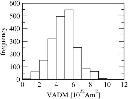
The Sint-2000 data comprises a time series of 2000 unsigned VADM values spaced by 1000 year, covering the past 2 Myr history of the geomagnetic dipole. The positions of the reversals are indicated in Figure 2 of Valet et al. (2005), where they show up as local minima in the VADM record. To obtain a VADM time series with sign we have inserted a sign change between those locations. The result is shown in Figure 1. In doing so we may miss some of the fine structure in the reversal time profile. However, in view of the considerable intrinsic uncertainties in the data [see Figure 2 of Valet et al. (2005)], similar and larger ambiguities apply to the whole VADM time series. The amplitude distribution of the unsigned VADM data is shown in Figure 2.
3 Method
We start with the discretized version of the Fokker-Planck equation. Discretization of space and time in Eq. 3 leads to
| (5) | |||||
We may rewrite this equation in matrix form as
| (6) |
where is a tridiagonal matrix with elements
| (7) |
By solving for and we obtain
| (8) |
These expressions will be used to infer and once the matrix has been determined.
Each column of adds up to zero, , so that there are two free parameters per spatial interval , exactly as many as the parameters and in the Fokker-Planck equation. An important consequence of the zero column sum is that Eq. (6) is norm-conserving,
| (9) |
In the limit Eq. (6) becomes
| (10) |
The object of this paper is to extract the effective position-dependent (= VADM-dependent) velocity and diffusion coefficient from a time series, in this case of the strength of the Earth’s magnetic dipole moment. To this end we construct from the data the matrix whose elements contain the transition probabilities for a system in position at some time to move to position at a later time . We begin by counting the number of times that the system is located in position at some time and in position at time . The required matrix elements are then equal to and have a statistical error . The normalization coefficients are fixed by the requirement that the columns of should add up to unity, . The time lag , finally, must be chosen comparable to, or larger than the correlation time of the randomly fluctuating part of the system, but small in comparison to the time scale on which the data changes systematically.
Our assumption is that the process is Markovian and therefore can be described by Eq. (10), from which it follows that . The theoretical transition matrix is therefore
| (11) |
and our goal is now to find a tridiagonal matrix such that closely resembles . The matrix has approximately degrees of freedom (ignoring boundary effects), of which can be eliminated by norm conservation (columns add up to zero). To find the remaining degrees of freedom we minimize the function
| (12) |
We could follow an alternative approach, by using the stationary distribution which we may find by binning the data as in Figure 2. Since the stationary distribution should obey Eq. (10), we have . This relation can be used to eliminate another degrees of freedom in , after which we find the remaining by minimizing the function (12). But we opted for fitting degrees of freedom and to use , or equivalently , as a consistency check on our computations.


4 Validation with the HD model
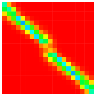
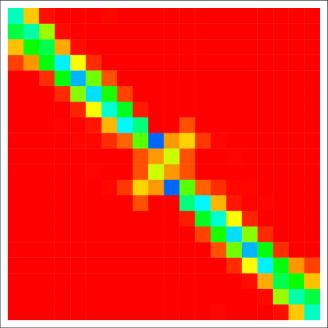
First, we test the approach outlined in the previous section on data generated with the model of Hoyng and Duistermaat (2004).333Henceforth referred to as ‘HD’ or ‘HD model’. This is a time series of VADMs measured in units of the equilibrium value, so corresponds to the nonlinear equilibrium value of the VADM. The series comprises data points with a time spacing of , and by construction this is also the correlation time.444The time resolution of this series is a factor 10 higher than that of the series used in Fig. 2 of HD, but the other parameters are the same (, , and ). Time is measured in units of the linear growth time of the dipole mode so that the series is about 50 Myr long in real time. We discretize the strength of the VADM into 25 bins of width 0.16 in dimensionless units, and we construct a histogram of all sets employing a time lag of . We then exploit the fact that there is no sign preference, that is, for a given realisation the series is an equally likely realisation. Accordingly, we add to the histogram all sets . We follow the procedure of the previous section, and the resulting effective transition matrix is plotted in Figure 3, left panel. Note that the blue matrix elements near the centre have a relatively large value but not a more accurate one: matrix elements near the centre of the figure are determined by small associated with reversals and these are rare. The most accurate elements correspond therefore to the equilibrium value , and are located in the wings near and in Figure 3 (left panel).
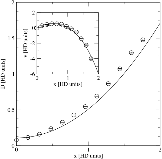
We then perform the fitting procedure outlined above to obtain the tridiagonal transition matrix , and in the right panel of Figure 3 we have plotted . There is a clear similarity between the two matrices. Figure 4 shows the resulting values for the diffusion coefficient and the effective growth rate (inset), computed with the help of (8). The error bars are 80% confidence intervals computed with the bootstrap method (Newman and Barkema, 1999). This captures the statistical errors, but not the systematic errors.
4.1 Comparison with theory
To place these results in perspective, we compute the Fokker-Planck equation for the probability density of by integrating Eqs. (5) and (6) of HD over the overtone amplitude , to find
| (13) |
Hence, we recover Eq. (3) with
| (14) |
Here a constant equal to for the HD dataset used here, and is the mean square overtone amplitude for given . The result is the two drawn lines in Figure 4. Since is only a weak function of , we did not bother to measure it from the simulation data. Instead, we replaced it by the average of over all , measured to be . The and recovered from the data compare rather well with their theoretical values (14). The agreement for could be further improved by allowing for the fact that is smaller than near and larger than for . However, we cannot expect agreement to within the statistical errors because of approximations made in deriving the Fokker-Planck equation (13). As a result there are small systematic differences between the statistical properties of predicted by (13) and (14) and those of the numerically generated . These differences are visible because we use many data points ().
These results demonstrate that our analysis is capable to extract the information on the effective VADM growth rate and the type of noise that was used to generate the time series. The scaling is a consequence of the multiplicative noise that the HD model employs [that is, a noise term of the type ]. But that is really a detail here. The main issue is that we have succesfully validated our retrieval method, as we have shown that our analysis is able to get out what has been put into the model. To avoid misunderstanding we note that this agreement does not say anything on whether the HD model describes the physics of the geomagnetic dipole correctly or not, or better than other reversal models do. It only tells us that our retrieval method appears to work satisfactorily.
5 Application to the Sint-2000 data
We then repeat the same procedure on the Sint-2000 data, Figure 1. The fitting procedure was performed with a time lag of kyr, see Figure 5. This choice is motivated as follows. The autocorrelation time of VADM data is a few hunderd yr (the time scale for rapid random changes in the geomagnetic dipole), but the sampling of the Sint-2000 VADM data increases that to 1 kyr. The time scale for systematic changes may be identified with the linear growth time of the dipole mode (of the order of 10 kyr). The resulting effective growth rate and diffusion coefficient are shown in Figure 6. The error bars are again 80% confidence intervals computed with the bootstrap method (Newman and Barkema, 1999). In reality, the errors will be larger as we did not allow for the considerable intrinsic errors in the VADM data (Valet et al., 2005).
The dependence of the effective growth rate is approximately as expected. The best fit of the function to the ‘data points’ yields ky, and Am2. For small we have which corresponds to linear growth of the dipole mode when it is small, and the term is the nonlinear quenching. The surprise is in the -dependence of the diffusion coefficient which we discuss below.

5.1 Implications for the geodynamo
The analysis of the Sint-2000 data confirms that the geomagnetic dipole mode is unstable with a linear growth time ky. The nonlinear quenching follows approximately a quadratic quenching function . The nonlinear equilibrium is attained at a VADM of Am2. These results are more or less as expected. To our knowledge this is the first time that the linear growth rate and the shape of the quenching function of the geomagnetic dipole have been measured from pertinent data.
In order to judge our results on the diffusion coefficient we derive the theoretical -dependence of . To this end we consider the induction equation of MHD: . The fluctuating velocity represents the convective turbulence in the metallic outer core superposed on a steady flow . If we expand the magnetic field in the induction equation in multipoles, the equation for the dipole becomes . Only the contribution of the fluctuating term acting on the dipole is written down explicitly. Comparing with Eq. (1) which produces a diffusion coefficient , we now obtain , where is the correlation time of , and the turbulent diffusion coefficient that occurs in the dynamo equation (Moffatt, 1978). Detailed considerations lead to (Hoyng, 2008)
| (15) |
where is the radius of the outer core and the number of convective cells in the core. There is a small, approximately constant contribution to due to feedback of the overtones on the dipole amplitude. This term also occurred in the HD model, cf. Eq. (14). It is important because it is related to the occurrence of reversals but it plays no role in the following discussion.
We expect therefore that , and the explanation is simple. The form of the induction equation makes that a given generates a change in proportional to the magnitude of . For given the diffusive motion of is therefore larger if is large, and this translates to the dipole component as well. However, these considerations are not borne out by our numerical results in Figure 6.
The increase of the diffusion coefficient for in Figure 6 is probably an artifact of the restricted length of the data, in combination with the fact that there are only five reversals and one aborted reversal in the last 2 Myr. VADMs smaller than Am2 are absent in the Sint-2000 data except during the very brief reversal periods. Since the data cannot resolve the fine structure of the VADM during a reversal one might wonder what the effect would be of a few rapid sign changes near a reversal, but that would only serve to make larger.
For VADM Am2 the diffusion coefficient is constant. In fact, one might say that the data are consistent with a constant at all VADM. We have tested the possibility that this result might somehow be caused by the limited time resolution of the Sint-2000 data. To this end we have generated from the HD data a Sint-2000-like series by taking a running average and then a subset of 2000 data points separated by 1000 yr. This can only be done approximately as we cannot convert the dimensionless time of the HD data (in units of the dipole growth time) into real time. It is conceivable that this new time series would have a large and a constant at larger , but the resulting and did not differ materially from those in Figure 4.
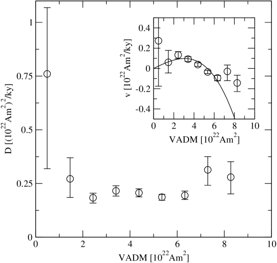
There seems to be no signature of multiplicative noise in the Sint-2000 data, and we believe that this is a solid result. Instead, the data indicate that the noise is quasi-additive, because the diffusion coefficient in Eq. (3) would be constant if in Eq. (1) is constant. We have no explanation for this, but there is the intriguing possibility that it is due to a nonlinear quenching of the fluid velocity fluctuations . If would scale as , then would be effectively independent of VADM, cf. (15). The best way to test these ideas would be to use a longer dataset, and an obvious possibility would be to use VADM data from hydromagnetic geodynamo simulations for this purpose.
6 Summary and conclusions
We have presented and validated a technique for extracting the effective growth rate and diffusion coefficient of a time series of a stochastic process. An attractive feature of the method is that it does not assume any a priori mathematical form for these quantities. Application of the method to the Sint-2000 VADM time series has shown that it is possible to measure the linear growth rate of the geomagnetic dipole and the shape of the nonlinear quenching of this growth rate. The dependence of the diffusion coefficient on the VADM suggests that the amplitude of the convective flows in the outer core is suppressed with increasing dipole strength. The main limitation in extracting more useful information on the geodynamo is the length of the Sint-2000 series. In future research, we will apply this analysis technique to time series obtained from hydromagnetic geodynamo simulations. If no nonlinear quenching is observed in these simulations, the simulation model produces time series which are qualitatively different from the Sint-2000 VADM time series. On the other hand, if these simulations show similar nonlinear quenching, then the cause of it can be investigated within the model.
Acknowledgements
We thank Dr. J.-P. Valet for making the Sint-2000 data available to us, and Prof. H. van Beijeren for helpful discussions.
References
Bouligand, C., Hulot, G., Khokhlov, A. and Glatzmaier, G.A., 2005. Statistical
paleomagnetic field modelling and dynamo numerical simulation. Geophys. J.
Int. 161, 603-626.
Christensen U., Olson, P. and Glatzmaier, G.A., 1999. Numerical modelling
of the geodynamo: a systematic parameter study. Geophys. J. Int. 138,
393-409.
Constable, C.G. and Parker, R.L., 1988. Statistics of the geomagnetic secular
variation in the past 5 Myr. J. Geophys. Res. 93, 11569-11581.
Gardiner, C.W., 1990. Handbook of Stochastic Methods. Springer-Verlag,
Berlin.
Glatzmaier, G.A. and Roberts, P.H., 1995. A three-dimensional
self-consistent computer simulation of a geomagnetic field reversal.
Nature 377, 203-209.
Guyodo, Y. and Valet, J.-P., 1999. Global changes in intensity of the
Earth’s magnetic field during the past 800 kyr. Nature 399, 249-252.
Hoyng, P., Schmitt, D. and Ossendrijver, M.A.J.H., 2002. A theoretical
analysis of the observed variability of the geomagnetic dipole field.
Phys. Earth Planet. Int. 130, 143-157.
Hoyng, P. and Duistermaat, J.J., 2004. Geomagnetic reversals and the
stochastic exit problem. Europhys. Lett. 68, 177-183. (HD)
Hoyng, P., 2008. To be submitted.
Hulot, G. and Le Mouël, J.L., 1994, A statistical approach to the
Earth’s main magnetic field. Phys. Earth Planet. Int. 82, 167-183.
Kuang, W. and Bloxham, J., 1997. An Earth-like numerical dynamo model.
Nature 389, 371-374.
Merrill, R.T., McElhinny, M.W. and McFadden, P.L., 1996. The Magnetic
Field of the Earth. Academic Press, New York.
Moffatt, H.K., 1978. Magnetic Field Generation in Electrically Conducting
Fluids. Cambridge U.P.
Newman, M.E.J. and Barkema, G.T., 1999. Monte Carlo Methods in Statistical
Physics. Oxford U.P.
Valet, J.-P., Meynadier, L. and Guyodo, Y., 2005. Geomagnetic dipole
strength and reversal rate over the past two million years. Nature 435,
802-805.
Van Kampen, N.G., 1992. Stochastic Methods in Physics and Chemistry.
North-Holland, Amsterdam.