Elemental abundances of Galactic bulge planetary nebulae from optical recombination lines

Abstract

Deep long-slit optical spectrophotometric observations are presented for 25 Galactic bulge planetary nebulae (GBPNe) and 6 Galactic disk planetary nebulae (GDPNe). The spectra, combined with archival ultraviolet spectra obtained with the International Ultraviolet Explorer (IUE) and infrared spectra obtained with the Infrared Space Observatory (ISO), have been used to carry out a detailed plasma diagnostic and element abundance analysis utilizing both collisional excited lines (CELs) and optical recombination lines (ORLs).

Comparisons of plasma diagnostic and abundance analysis results obtained from CELs and from ORLs reproduce many of the patterns previously found for GDPNe. In particular we show that the large discrepancies between electron temperatures ($T_{\rm e}$’s) derived from CELs and from ORLs appear to be mainly caused by abnormally low values yielded by recombination lines and/or continua. Similarly, the large discrepancies between heavy element abundances deduced from ORLs and from CELs are largely caused by abnormally high values obtained from ORLs, up to tens of solar in extreme cases. It appears that whatever mechanisms are causing the ubiquitous dichotomy between CELs and ORLs, their main effects are to enhance the emission of ORLs, but hardly affect that of CELs. It seems that heavy element abundances deduced from ORLs may not reflect the bulk composition of the nebula. Rather, our analysis suggests that ORLs of heavy element ions mainly originate from a previously unseen component of plasma of $T_{\rm e}$’s of just a few hundred Kelvin, which is too cool to excite any optical and UV CELs.

We find that GBPNe are on the average 0.1–0.2 dex more metal-rich than GDPNe but have a mean C/O ratio that is approximately 0.2 dex lower. By comparing the observed relative abundances of heavy elements with recent theoretical predictions, we show that GBPNe probably evolved from a relatively metal-rich environment of initial $Z\sim 0.013$, compared to an initial $Z\la 0.008$ for GDPNe. In addition, we find that GBPNe tend to have more massive progenitor stars than GDPNe. GBPNe are found to have an average magnesium abundance about 0.13 dex higher than GDPNe. The latter have a mean magnesium abundance almost identical to the solar value. The enhancement of magnesium in GBPNe and the large [$\alpha$/Fe] ratios of bulge giants suggest that the primary enrichment process in the bulge was Type II SNe. PN observations yield a Ne/O abundance ratio much higher than the solar value, suggesting that the solar neon abundance may have been underestimated by 0.2 dex.

1 Introduction

Knowledge of the chemical composition of the Galactic bulge is of paramount importance for the understanding of the history of formation and evolution of the Galaxy (e.g. van den Bergh1996; McWilliam1997). While early work suggested that bulge stars are super metal-rich (eg. Whitford & Rich1983; Rich1988; Geisler & Friel1992), more recent high resolution spectroscopic studies showed that the bulge is actually slightly iron-poor compared to the solar neighborhood (McWilliam & Rich1994), a result supported by the analysis of low resolution spectroscopic and photometric observations for a large sample of bulge K and M giants by (Ibata & Gilmore1995). In addition, a careful metallicity analysis of low resolution spectra of integrated light from the Galactic bulge in Baade’s window by Idiart et al. (1996) suggested that the bulge is enhanced in $\alpha$-elements (represented by magnesium).

All the aforementioned studies were based on analysis of light from bulge stars and yielded essentially no information of abundances of light elements such as carbon and oxygen. In this context, abundance analyses using GBPNe as probes can play an important role. Planetary nebulae (PNe) are products of low- and intermediate-mass stars (LIMS). Ionizing stars of PNe have typical luminosities of several hundreds to thousands solar luminosity. Much of the energy is emitted in a few strong narrow emission lines, making them easily observable to large distances. In the optical and infrared, many PNe in the Galactic bulge can be readily observed even though the bulge is heavily obscured by intervening dust grains in the Galactic disk. For most elements, PNe are believed to preserve much of the original composition of the interstellar medium (ISM) at the time of their formation. Elemental abundances derived from PN observations can therefore be compared and related to results from stellar abundance analyses. Possible exceptions are light elements such as He, N and C, whose abundances can potentially be modified by various dredge-up processes, depending on mass and initial metallicity of the progenitor star. Measurements of abundances of those elements in PNe thus shed light on the nucleosynthesis and dredge processes that occurred during the late evolutionary stages of their progenitor stars.

Hitherto, spectroscopic abundance determinations have been carried out for approximately 250 GBPNe. The analyses were almost invariably based on observations of relatively strong CELs (Ratag et al.1992, Ratag et al.1997; Escudero et al. 2004; Exter et al. 2004). The results show that, albeit with large scatter, GBPNe have average abundances and abundance distributions similar to GDPNe for elements unaffected by evolution of their progenitor stars, such as oxygen and other heavier elements. For helium and nitrogen, whose abundances may have been altered by the various dredge-up processes, studies so far have yielded different results. Part of the discrepancies may be due to differences in PN populations sampled by individual studies.

The heavy extinction towards the Galactic bulge prohibits extensive ultraviolet (UV) spectroscopy of GBPNe. Only a very restrictive number of UV spectra, obtained mainly with the IUE, are available for GBPNe, mostly located within Baade’s window. This poses a serious limitation for the study of some key elements, such as carbon for which the only observable strong CELs, the C iv $\lambda\lambda$1548,1550 and C iii] $\lambda\lambda$1907,1909 lines, fall in the ultraviolet (the infrared [C ii] 158$\mu$m line arises mainly from the photodissociation region surrounding the ionized region, rather than from the latter itself). As a consequence, very little is known at the moment about the abundance and its distribution of this key element for the bulge population. Even with suitable UV observations, the analysis is complicated by the uncertain extinction law towards the Galactic bulge, which is known to deviate from that of the general ISM of the Galactic disk (Walton, Barlow & Clegg 1993; Liu et al. 2001).

Advances in the past decade in observational techniques and in calculations of the basic atomic data, such as effective recombination coefficients for non-hydrogenic ions with multiple valence electrons, have made it possible to determine nebular abundances using faint optical recombination lines from heavy element ions (e.g. Liu et al. 1995, 2000, 2001). Ionic abundances deduced from ORLs have the advantage that they are almost independent of the physical conditions, such as $T_{\rm e}$  and electron density ($N_{\rm e}$), of the nebula under study. Dominant ionic species of carbon typically found in photoionized gaseous nebulae possess a number of relatively bright ORLs, such as C ii $\lambda$4267, C iii $\lambda$4187 and $\lambda$4650 and C iv 4658 (blended with the [Fe iii] $\lambda$4658 line in some objects), allowing measurements of ionic abundances of C²⁺, C³⁺ and C⁴⁺. These lines are routinely detected in spectra of reasonable quality for bright Galactic PNe (e.g. Liu 1998).

Deep, medium resolution optical spectroscopy, allowing determinations from ORLs of abundances of carbon, nitrogen, oxygen and neon, have been carried out for several dozen GDPNe (Tsamis et al. 2003, 2004; Liu et al. 2004a,b; Wesson, Liu & Barlow 2005). It is found that ionic abundances derived from ORLs are ubiquitously higher than values derived from CELs, i.e. abundance discrepancy factor (adf) $\ga 1$ for all the nebulae analyzed so far. The adf is found to vary from nebula to nebula and typically falls in the range 1.6–3.0, but with a significant tail extending to much higher values, reaching 70 in the most extreme case found so far (c.f. Liu 2003, 2006b for recent reviews). On the other hand, analyses also show that for a given nebula, adf’s derived for all abundant second-row elements, C, N, O and Ne, are of similar magnitude; in other words, heavy element abundance ratios, such as C/O, N/O and Ne/O are unaffected, regardless of the actual value of the adf (Liu et al. 1995, 2000, 2001; Mathis et al. 1998; Luo et al. 2001; Tsamis et al. 2004; Liu et al. 2004b). In stark contrast to those abundant second-row elements, ORL abundance determinations for magnesium, the only third-row element that has been studied using an ORL, yield nearly a constant Mg/H abundance ratio almost identical to the solar value (Barlow et al. 2003; Liu 2006b).

Detailed plasma diagnostics using ORLs indicate that ORLs may originate in regions of $T_{\rm e}$  and $N_{\rm e}$  quite different from those where CELs are emitted. While new observations have confirmed the earlier results of (Peimbert1971) and Liu & Danziger (1993) that $T_{\rm e}$’s, derived from the Balmer discontinuity of the hydrogen recombination spectrum are systematically lower than values deduced from the collisionally excited [O iii] nebular to auroral forbidden line ratio, careful analyses of the relative intensities of He i ORLs suggest that He i ORLs may arise from plasmas of $T_{\rm e}$’s even lower than indicated by the H i Balmer discontinuity. Much more importantly, careful comparisons of high quality measurements of observed relative intensities of O ii ORLs in spectra of PNe exhibiting particularly large adf’s ($\ga 5$) clearly show that the lines arise from plasmas of $T_{\rm e}$ $\sim 1000$ K, about an order of magnitude lower than values deduced from the [O iii] forbidden line ratios. The observations thus point to the presence of another component of cold plasma, previously unknown, embedded in the diffuse nebula. The gas has much higher metallicity and, because of the much enhanced cooling, a much lower $T_{\rm e}$. In addition, because of the very low $T_{\rm e}$, much lower than the typical excitation energies of optical and UV CELs, it emits essentially no optical and UV CELs, and is thus invisible via those lines. The existence of such a cold, H-deficient component of plasma thus provides a natural explanation for the systematic higher heavy elemental abundances and lower $T_{\rm e}$’s deduced from ORLs compared to those derived from CELs (Liu et al. 2000, 2006). The nature and origin of the high-metallicity gas remain elusive. Accurate determinations of the prevailing physical conditions ($T_{\rm e}$  and $N_{\rm e}$) and elemental abundances will be essential.

In this paper, we present deep, high-quality optical spectra for a sample of 25 GBPNe plus 6 GDPNe. The data are combined with archival IR and UV spectra to study the nebular physical conditions and elemental abundances using both CELs and ORLs. The sample, together with those published previously, mainly for GDPNe, bring the total number of PNe for which ORL elemental abundances have been determined to nearly a hundred. The purposes of the study are two folds: 1) to determine and characterize the distribution of adf’s for a significant sample of GBPNe and compare it to that for GDPNe; 2) to determine carbon abundances and C/O ratios for the first time for a significant sample of GBPNe which are poorly known for the bulge population. The paper is organized as follows. In Section 2, we describe briefly our new optical observations and archival IR and UV data. Plasma diagnostics, ionic and elemental abundance determinations using CELs and ORLs are presented respectively in Sections 3 and 4. In Section 5, we compare our results with those in the literature. In Section 6, we present a statistical analysis of adf’s and other nebular physical properties. In Section 7, we contrast the abundance patterns deduced for GDPNe and for GBPNe and compare them to theoretical models. We conclude by summarizing the main results in the last Section.

Table 1: Basic data. Angular diameters are optical measurements except as specified.

Name	PNG	Diam	$-$log$F(\rm H\beta)$		$F$(5 GHz)	RV	B	V
		($\arcsec$)	(erg cm-2 s-1)		(mJy    )	(km s-1)	(mag)	(mag)
		A92	CKS92	WL07		D98	T91,T89
Bulge PNe
Cn 1-5	002.2$-$09.4	7.0	11.25	11.40	44.0	$-$29	15.50	15.20
Cn 2-1	356.2$-$04.4	2.4	11.64	11.63	49.0	$-$271	*	*
H 1-41	356.7$-$04.8	9.6	11.7a	11.90	12.0	76	16.30	16.20
H 1-42	357.2$-$04.5	5.8	11.7a	11.68	40.0	$-$79	17.30	*
H 1-50	358.7$-$05.2	1.4b	11.68	11.70	31.0	28	*	17.10
H 1-54	002.1$-$04.2	4.8	11.89	11.87	31.0	$-$116	15.70	15.40
IC 4699	348.0-13.8	5.0	11.69	11.70	20.0	$-$123	14.82	15.10
M 1-20	006.1+08.3	1.9c	11.93	11.94	51.0	91	17.70	17.10
M 2-4	349.8+04.4	5.0	11.84	11.94	32.0	$-$184	17.60	17.00
M 2-6	353.3+06.3	8.0	12.16	12.23	17.0	$-$88	16.67	16.40
M 2-23	002.2$-$02.7	8.5	11.58	11.58	41.0	224	16.70	*
M 2-27	359.9$-$04.5	4.8	12.21	12.23	50.0	170	*	*
M 2-31	006.0$-$03.6	5.1	12.11a	12.10	51.0	157	*	*
M 2-33	002.0$-$06.2	5.8	11.6a	11.85	12.0	$-$112	14.40	14.40
M 2-39	008.1$-$04.7	3.2	12.13	12.07	8.0	71	16.20	15.80
M 2-42	008.2$-$04.8	3.8	12.12	12.10	14.0	157	18.20	*
M 3-7	357.1+03.6	5.8	12.32	12.38	28.0	$-$191	17.30	16.40
M 3-21	355.1$-$06.9	5.0d	11.42	11.39	30.0	$-$68	16.20	15.30
M 3-29	004.0-11.1	8.2	11.7a	11.78	12.0	50	15.42	15.50
M 3-32	009.4$-$09.8	6.0	11.9a	11.85	12.0	46	17.40	17.10
M 3-33	009.6-10.6	5.0	12.00	11.93	7.5	173	15.70	15.90
NGC 6439	011.0+05.8	5.0	11.71	11.73	55.0	$-$93	20.20	*
NGC 6565	003.5$-$04.6	13.6	11.22	11.25	38.2	$-$20	*	18.50
NGC 6620	005.8$-$06.1	8.0	11.74	11.73	3.5	72	*	19.60
VY 2-1	007.0$-$06.8	7.0d	11.50	11.57	37.0	115	16.60	*
Disk PNe
H 1-35	355.7$-$03.5	2.0	11.52	11.50	72.0	160	15.70	15.40
M 1-29	359.1$-$01.7	7.6	12.2a	12.41	97.0	-62	*	*
M 1-61	019.4$-$05.3	1.8c	11.43	11.46	97.0	40	17.10	*
NGC 6567	011.7$-$00.6	7.6	10.95	10.94	76.0	119	14.42	14.36
He 2-118	327.5+13.3	5.0	11.70	11.67	10.0d	$-$164	18.20	18.70
IC 4846	027.6$-$09.6	2.0	11.34	11.30	43.0	151	15.19	15.19

• A92 - Acker et al. (1992); CKS92 - (Cahn et al.1992); D98 - (Durand et al.1998); T89 - Tylenda et al. (1989); T91 - (Tylenda et al.1991); WL07 - from long-slit observations of the current work

• From Acker et al. (1992).

• Radio measurement from (Zijlstra et al.1989).

• Radio measurement from Aaquist & Kwok (1990).

• Upper limit.

2 Targets and Observations

In total 31 PNe in the direction of the Galactic center were observed. The basic parameters of the targets, including observed absolute H$\beta$ flux, radio flux density at 5.0 GHz, angular diameter (value measured in the optical is adopted if available, otherwise radio measurement is used), heliocentric radial velocity and magnitude of the central star are given in Table 1. We assume that a PN probably belongs to the bulge population if it falls within 20 degrees of the Galactic center, has an angular diameter less than 20″, a 5 GHz radio flux density of less than 50 mJy and a relatively large heliocentric radial velocity (, Ratag et al.1997). 25 of our targets satisfy these criteria. For the remaining 6 nebulae, H 1-35, M 1-29, M 1-61 and NGC 6567 have a radio flux density in excess of 70 mJy, and IC 4846 and He 2-118 fall nearly 30 degrees or more from the Galactic center. They are thus more likely belonging to the disk rather than the bulge population. We include these six PNe in our sample of GDPNe (c.f. Section 7).

2.1 Optical observations

Table 2: Journal of ESO 1.52-m observations.

Name	Date	$\lambda$-range	FWHM	Exp. Time
	(UT)	(Å)	(Å)	(sec)
Cn 1-5	07/1996	3520–7420	4.5	30,300
	07/1995	3994–4983	1.5	2$\times$1200
Cn 2-1	07/1995	3520–7420	4.5	15,300
	07/1995	3994–4983	1.0	2$\times$1800
	06/2001	3500–4805	1.5	1200
H 1-35	07/1995	3520–7420	4.5	30,300
	07/1996	3994–4983	1.0	2$\times$1800
	06/2001	3500–4805	1.5	1200
	06/2001	4660–7260	3.0	900
H 1-41	07/1995	3520–7420	4.5	30,2$\times$300
	07/1996	3994–4983	1.5	2$\times$1200
H 1-42	07/1995	3520–7420	4.5	30,300
	07/1996	3994–4983	1.0	2$\times$1800
H 1-50	07/1995	3520–7420	4.5	30,300
	07/1995	3994–4983	1.0	2$\times$1800
	06/2001	3500–4805	1.5	1200
H 1-54	07/1996	3527–7431	6.0	60,300
	07/1996	3994–4983	1.5	2$\times$1800
	06/2001	4660–7260	1.5	900
He 2-118	07/1996	3520–7420	4.5	30,300
	07/1995	3994–4983	1.5	2$\times$1200
	06/2001	3500–4805	1.5	1200
IC 4699	07/1995	3520–7420	4.5	90,300
	07/1995	3993–4979	0.9	2$\times$1800
IC 4846	07/1995	3520–7420	4.5	30,300
	07/1995	3993–4980	0.9	2$\times$1800
M 1-20	07/1996	3527–7431	6.0	60,300
	07/1996	3994–4984	1.5	2$\times$1800
	06/2001	3500–4805	1.5	1800
M 1-29	07/1996	3527–7431	6.0	60,600
M 1-61	07/1995	3520–7420	4.5	20,300
	07/1995	3993–4980	0.9	300,2$\times$1800
M 2-4	07/1995	3520–7420	4.5	30,300
	07/1996	3994–4984	1.5	2$\times$1800
	06/2001	3500–4805	1.5	1800
M 2-6	07/1996	3520–7420	6.0	30,300
	07/1996	3994–4984	1.5	1800
M 2-23	07/1995	3520–7420	4.5	15,300
	07/1996	3994–4984	1.5	2$\times$1500
M 2-27	07/1996	3527–7431	6.0	60,600
M 2-31	07/1996	3527–7431	6.0	60,300
M 2-33	07/1996	3527–7431	6.0	60,300
	07/1996	3994–4984	1.5	2$\times$1800
M 2-39	07/1995	3520–7420	4.5	120,300
	07/1996	3994–4984	1.5	2$\times$1800
M 2-42	07/1996	3520–7431	6.0	60,300
M 3-7	07/1996	3527–7431	6.0	60,300
M 3-21	07/1995	3520–7420	4.5	10,300
	07/1996	3994–4984	0.9	2$\times$1800
	06/2001	3500–4805	1.5	2$\times$1200
M 3-29	07/1996	3520–7431	6.0	60,300
M 3-32	07/1995	3530–7430	4.5	60,2$\times$300
	07/1996	3030–4050	1.5	2$\times$1800
	07/1996	3990–5000	1.5	2$\times$1800
M 3-33	07/1995	3520–7420	4.5	60,300
	07/1996	3994–4984	1.5	2$\times$1800
NGC 6439	07/1995	3520–7420	4.5	30,300
	07/1996	3994–4983	1.5	2$\times$1200
	06/2001	3500–4805	1.5	1200,2$\times$1800
NGC 6565	07/1995	3520–7420	4.5	90,300
	07/1995	3993–4979	0.9	2$\times$1800

Table 2: –continued

Name	Date	$\lambda$-range	FWHM	Exp. Time
	(UT)	(Å)	(Å)	(sec)
NGC 6567	07/1995	3520–7420	4.5	20,300
	07/1995	3900–4980	0.9	600,2$\times$1800
	06/2001	3500–4805	1.5	1200
NGC 6620	07/1995	3520–7420	4.5	60,300
	07/1995	4000–4987	0.9	2$\times$1800
	06/2001	3500–4805	1.5	3$\times$1800
VY 2-1	07/1995	3520–7420	4.5	30,300
	07/1996	3994–4984	1.5	2$\times$1800

The spectra were obtained in 1995, 1996 and 2001 with the European Southern Observatory (ESO) 1.52 m telescope using the Boller & Chivens (B&C) long-slit spectrograph. A journal of observations is presented in Table 2. In 1995, the spectrograph was equipped with a Ford 2048$\times$2048 $15\,\mu{\rm m}\times 15\,\mu{\rm m}$ CCD, which was superseded in 1996 by a UV-enhanced Loral $2048\times 2048$ $15\,\mu{\rm m}\times 15\,\mu{\rm m}$ chip and in 2001 by a Loral $2688\times 2688$ $15\,\mu{\rm m}\times 15\,\mu{\rm m}$ chip.

Two grating setups were used. The low resolution setting yielded a FWHM of $\sim 4.5$ or 6.0 Å and covered the wavelength range from 3520 Å to 7420 Å. The high resolution setting gave a full width half maximum (FWHM) of $\sim 0.9$ or 1.5 Å and covered the wavelength range 3994 – 4983 or 3500 – 4800 Å. Typical exposure times were about 5 min for the low resolution setting. For the high spectral resolution, integration times of 20 to 30 min were used, and in most cases two or more frames were taken to increase the signal-to-noise (S/N) ratio and to facilitate removal of cosmic rays. The observations were aimed to detect at least the strongest ORLs of O ii, i.e. the $\lambda$4649 line from Multiplet V 1. In order to obtain strengths of the very strong emission lines, such as [O iii] $\lambda\lambda$4959, 5007 and H$\alpha$ which saturated on long exposures, short exposures of duration of 10 to 60 seconds were also obtained. A slit width of 2″ was used for all nebular observations. However, in order to obtain the total flux of H$\beta$, a short exposure was taken using an 8″ wide slit for each nebula for the low spectral resolution setup.

All nebulae were observed with a fixed position long-slit, normally passing through the nebular center and sampling the brightest parts of the nebula. The only exception was Cn 1-5 for which scanned spectra were obtained by uniformly driving a long slit across the nebular surface, thus yielding average spectra for the entire nebula.

All the two-dimensional long-slit spectra were reduced using the long92 package in midas following the standard procedure. Spectra were bias-subtracted, flat-fielded and cosmic-rays removed, and then wavelength calibrated using exposures of a calibration lamp. Flux-calibration was carried out using the IRAF package by using wide-slit spectroscopic observations of HST standard stars.

The 3.5 arcmin long-slit was long enough to cover the entire nebula for all sample objects while still leaving ample clear area to sample the sky background. The sky spectrum was generated by choosing sky windows on both sides of the nebular emission while avoiding regions of background/foreground stars. The sky spectrum was then subtracted from the two-dimensional spectrum. After sky-subtraction, the two-dimensional spectra were integrated along the slit direction over the nebular surface. For a few nebulae with a bright central star, such as NGC 6567 and M 2-33, a few CCD rows centered on the star were excluded in the summation to avoid strong contamination of the stellar light.

As an example illustrating the high quality of our data, we plot in Fig. 1 the spectra of M 3-32 and M 3-21 from 3520 to 4980 Å after integration along the slit. Also overplotted in Fig. 1 is a synthetic spectrum for M 3-21, which includes contribution from recombination lines and continua of H i, He i and He ii as well as from CELs and ORLs emitted by ionized carbon, nitrogen, oxygen and neon ions, assuming $T_{\rm e}$  and $N_{\rm e}$  as well as ionic abundances deduced in Sections 3 and 4.

All fluxes were measured on sky-subtracted and extracted one-dimensional spectra, using techniques of Gaussian line profile fitting in midas. For the strongest lines, however, fluxes obtained by simply integrating over the observed line profile were adopted.

H$\beta$ fluxes derived from our wide slit observations are listed in Table 1 and compared to values published in the literature. In Fig. 2, we compare our own measurements with those compiled by (Cahn et al.1992). The agreement is quite good except for a few nebulae of angular diameters larger than 8″. For those large PNe, our measurements should be treated as lower limits.

Most ORLs from CNONe ions are quite weak and often blend together (c.f. Fig. 1). To retrieve their intensities, multiple Gaussian fitting was used. Given that the typical expanding velocity of a PN is $<25$ km s^-1 (e.g. Kwok1994), much smaller than the width of instrumental broadening ($\sim$ 55 km s^-1 at H$\beta$ for a FWHM of 0.9 Å, the best resolution of our optical spectra), all lines detected with the same instrument setup were thus assumed to have the same line width, which was dominated by instrumental broadening. This assumption, together with accurately known laboratory wavelengths of identified lines, significantly reduce the number of free (non-linear) parameters when fitting blended lines using multiple Gaussian. Apart from this procedure, synthetic spectra (c.f. Section 3.1), were also used to aid line identifications and flux measurements in cases of serious line blending. The measured line fluxes, normalized such that $F({\sc H}\beta)=100$, are presented in Appendix A, Table 15. Fluxes of lines measured on high resolution blue spectra were normalized to H$\beta$ via H$\gamma$, the flux of the latter relative to H$\beta$ was obtained from low resolution spectra which covered nearly the whole optical wavelength range.

Given the weakness of the nebular continuum and high-order Balmer lines, and the fact that as $n$, the principal quantum number of the upper level, approaches 20, high-order Balmer lines start to blend together, good S/N’s and spectral resolution are essential for accurate measurements of the Balmer discontinuity and decrement, and consequently for accurate determinations of the Balmer jump temperature, $T_{\rm e}$(BJ), and Balmer decrement density, $N_{\rm e}$(BD) (c.f. Section 3.4). Among our sample of 31 PNe, deep high resolution spectra in the blue that cover the wavelength region of the Balmer discontinuity and high-order Balmer lines near 3646Å  are available for 8 GBPNe and 3 GDPNe. In subsequent analysis, we shall call this sub-sample of PNe as ‘A’ and the remaining nebulae (including 17 GBPNe and 3 GDPNe) as sub-sample ‘B’. For PNe of sub-sample B, values of $T_{\rm e}$(BJ) and $N_{\rm e}$(BD) determined are quite uncertain. Fortunately, given the fact that emissivities of ORLs have only a weak power-law dependence on $T_{\rm e}$, quite similar to that of H i Balmer lines, and are nearly independent on $N_{\rm e}$  at low densities ($N_{\rm e}\la 10^{6}$ cm^-3), the effects of uncertainties in $T_{\rm e}$(BJ) and $N_{\rm e}$(BD) on ionic abundances deduced from ORLs are minimal (c.f. Section 4.2).

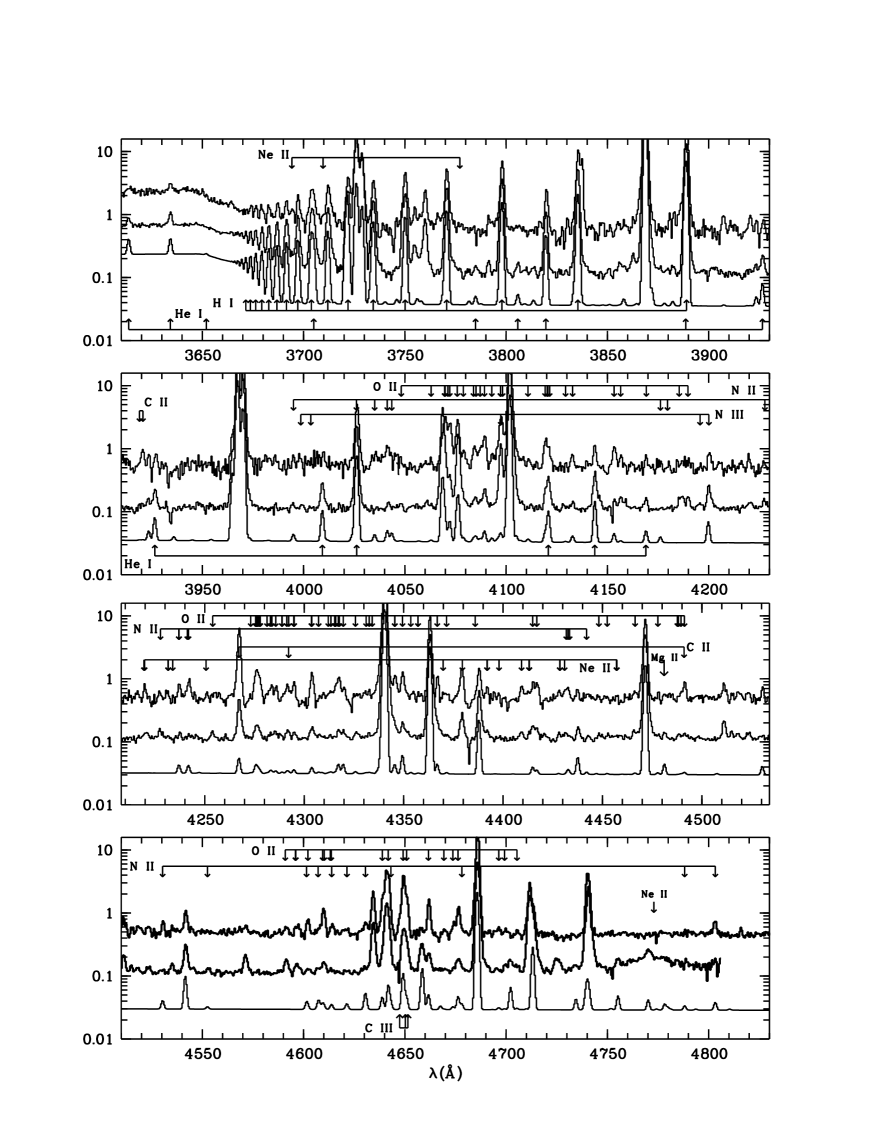
Figure 1: Optical spectra of M 3-32 (upper curve, scaled up by a factor of 2.5) and M 3-21 (middle curve, scaled up by a factor of 1.5) from 3520 – 4980 Å, showing the rich recombination lines from H i, He i and He ii as well as C ii, N ii, O ii, Ne ii. Also overplotted is a synthetic spectrum for M 3-21 (lower curve), which includes contribution of recombination continuum and line emission from hydrogen and helium as well as CELs and ORLs from CNONe ions. The observed spectra have been corrected to laboratory wavelengths using H i Balmer lines and normalized such that $I({\rm H}\beta)=100$. The spectra have also been corrected for interstellar extinction.

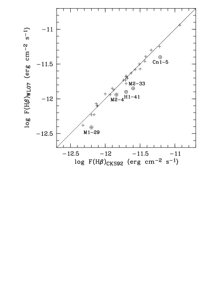
Figure 2: H$\beta$ fluxes derived from our own observations taken with an 8″ slit width (ordinate) are compared to values published in the literature as compiled by (Cahn et al.1992) (abscissa). The five nebulae for which our measurements are more than 10 per cent lower than those given in (Cahn et al.1992) are marked with open circles and labelled by their names.

For a few PNe such as M 2-27 in our sample, only low resolution spectra were available. Given the low spectral resolution and S/N ratio, the data were insufficient to deblend and measure weak lines. In those cases, synthetic spectra were used to fit the spectra in order to obtain crude estimates of $T_{\rm e}$, $N_{\rm e}$  and abundances from ORLs.

2.2 UV observations

Table 3: Journal of IUE observations.

Name	Data set	Exp. Time
		(sec)
Cn 1-5	SWP 39446	3000
	SWP 39455	6000
	LWP 18567	4000
	LWP 18577	3000
H 1-42	SWP 39447	12840
H 1-50	SWP 54686	23100
IC 4846	SWP 33381	3600
	LWP 13130	4800
M 2-23	SWP 44207	25380
M 2-33	SWP 55509	24000
M 2-39	SWP 33396	8580
M 3-21	SWP 39464	8460
	SWP 39465	10800
M 3-29	SWP 30480	1500
	SWP 54464	8400
M 3-32	SWP 54726	24000
	SWP 55541	24000
M 3-33	SWP 44199	7200
NGC 6439	SWP 55484	19200
NGC 6565	SWP 07984	2100
	SWP 35690	9000
	SWP 24266	3600
	LWP 04611	3600
	LWR 06955	2100
	LWP 15144	9000
NGC 6567	SWP 17019	11160
	SWP 45362	7200
	SWP 45381	1320
	LWR 13307	3600
	LWP 23708	3600
NGC 6620	SWP 45836	1800
	SWP 48320	8760
	SWP 54512	2400
	SWP 54700	3300
Vy 2-1	SWP 44200	12240

Sixteen among the 31 PNe have been observed with the IUE in the ultraviolet. The data were retrieved from the INES Archive Data Server in Vilspa, Spain, processed with the final (NEWSIPS) extraction method. All spectra were obtained with the SWP and LWP/LWR cameras using the IUE large aperture, a $10.3\arcsec\times 23\arcsec$ oval, large enough to encompass all PNe of the current sample. The wavelength coverages of SWP and LWP/LWR spectra are from 1150–1975 and from 1910–3300 Å, respectively. When several spectra for a given nebula were available, they were co-added weighted by integration time. The UV fluxes were normalized to $F({\rm H}\beta)=100$ using the absolute H$\beta$ fluxes tabulated in Table 1. Absolute H$\beta$ fluxes compiled by CKS92 were adopted, except for objects without published reliable measurement, for which our own measurements were used (c.f. Section 2.1 and 3.1). A journal of IUE observation is given in Table 3. Corrections for interstellar extinction will be discussed in Section 3.1.

Several emission lines from highly-ionized species, such as N v $\lambda$1240, have been detected in the IUE SWP spectrum of the medium excitation class PN Cn 1-5. The nebula has a Wolf-Rayet central star (Acker & Neiner 2003). The lines show clearly P-Cygni profiles and therefore most likely originate from wind emission of the central star. Its optical spectrum yields a He ii $\lambda 4686$ intensity of 0.9 on the scale where $F({\rm H}\beta)=100$. The measurement was quite uncertain as the 4570 – 4720 Å spectral region was severely contaminated by strong WR features from C iii and C iv. At $T_{\rm e}=10\,000$ K, the He ii $\lambda 1640$/$\lambda$4686 intensity ratio has a predicted value of 6.6. The measured optical flux of the He ii $\lambda 4686$ line then implies a $\lambda 1640$ line flux of 6, which is a factor of ten lower than measured from the IUE spectrum (after reddening corrections). This shows that He ii emission detected in the IUE spectrum is indeed dominated by wind emission, rather than from the gaseous envelope. In Section 4, we will use the observed intensity of the He ii $\lambda 4686$ to obtain an estimate of the He⁺⁺/H⁺ abundance for the gaseous envelope of this PN. We also note that the blue absorption is quite weak for the C iv $\lambda$1550 feature and its observed flux will be used to obtain a rough estimate of the C³⁺/H⁺ ionic abundance for this PN.

2.3 Infrared observations

Three objects in our sample were observed with the Short Wavelength Spectrometer (SWS) and Long Wavelength Spectrometer (LWS) on board ISO. Cn 1-5 has one SWS01 and one LWS01 spectrum available. The SWS01 spectrum covered the 2.4–45 $\mu$m wavelength range at a FWHM of approximately 0.3 $\mu$m, whereas the LWS01 covered from 43–197 $\mu$m at a FWHM of about 0.6 $\mu$m. For M 2-23, several lines in the SWS wavelength range were scanned using the SWS02 mode, which yielded a spectral resolving power between 1000 and 4000, depending on wavelength as well as on source angular extension. Finally the SWS02 and LWS02 observing modes were used to scan a number of lines in NGC 6567 in both the SWS and LWS wavelength ranges.

The angular sizes of the three nebulae are small enough such that both SWS and LWS observations should capture the total flux from the entire nebula. Line fluxes measured from the infrared spectra were normalized to $F({\rm H}\beta)=100$ via the absolute H$\beta$ flux listed in Table 1 which were compiled by CKS92. The normalized line fluxes are listed in Table 16 and then dereddened as discussed in the next Section.

3 Nebular analysis

Our analyses follow closely the procedures outlined in Liu et al. (2001) who presented detailed studies of two GBPNe, M 1-42 and M 2-36. Firstly, extinction curves towards individual sightlines were derived from radio continuum flux density and H i, He i and He ii recombination lines. Plasma diagnostic analyses were then carried out using both CELs and ORLs, followed by ionic and total elemental abundance determinations.

3.1 Extinction correction

Before any nebular analyses, measured line fluxes need to be corrected for effects of extinction by intervening dust grains along the sightline. Some PNe, such as the nearby NGC 7027 and NGC 6302, are also known to harbour large amounts of local dust (Seaton 1979; Middlemass 1990; Lester & Dinerstein 1984). For GDPNe, it is generally sufficient to use the standard Galactic extinction law for the general diffuse ISM, which has a total-to-selective extinction ratio $R_{\rm v}=A({\rm V})/E_{\rm B-V}=A({\rm V})/[A({\rm B})-A({\rm V})]$ = 3.1 (c.f. Howarth1983; H83 hereafter). In that case, the amount of extinction can be characterized by a single parameter, the logarithmic extinction at H$\beta$, $c({\rm H}\beta)$. However, large variations in reddening curves towards individual sightlines are also observed, particularly in the UV (Massa & Savage1989). It is found that the linear rise of extinction in the far-UV decreases dramatically with $R_{\rm v}$ and suggests that in dense regions, carriers of the far-UV extinction, including those of the 2175 Å bump reside in large grains (Cardelli et al. 1989). Earlier work on extinction towards the Galactic bulge in the optical and UV region indicates a steep reddening law in the UV, with values of $R_{\rm v}$ ranging from 1.75 to 2.7 (Walton et al.1993; Ruffle et al.2004).

Liu et al. (2001) derived extinction curves towards M 1-42 and M 2-36 by comparing the observed Balmer decrement, the He ii $\lambda 1640/\lambda 4686$ and $\lambda 3203/\lambda 4686$ ratios, and the ratio of total H$\beta$ flux to radio f-f continuum flux density with the predictions of recombination theory (Storey & Hummer1995). In the current work the same method was adopted. Firstly, intrinsic intensities $I(\lambda)$ of H i Balmer lines were calculated from the radio continuum flux density at 5 GHz or 1.4 GHz, assuming that the nebula is optically thin at those frequencies. Comparison between the predicted and observed fluxes of individual lines yields the extinction value $A(\lambda)$ at the wavelength of the line. Similarly, from the observed He ii$\lambda$1640/4686 ratio, the differential extinction between the two wavelengths, $A(\lambda 1640)-A(\lambda 4686)$, can be derived. The value, when combined with $A(\lambda 4686)$, obtained by interpolating $A(\lambda 4340)$ and $A(\lambda 4861)$, then yields $A(\lambda 1640)$. In this way, extinction values at a set of wavelengths can be established, allowing characterization of the extinction law towards individual objects.

Since the ratio of the radio continuum flux density to F(H$\beta$) depends weakly on $T_{\rm e}$  and helium ionic abundances, a preliminary plasma diagnostic and abundance analysis were carried out assuming the standard ISM reddening law (Howarth1983). Radio flux densities at 1.4 GHz for our sample nebulae were mostly taken from Condon & Kaplan (1998), whereas those of 5 GHz were mainly from (Zijlstra et al.1989). For total H$\beta$ flux, $F({\rm H}\beta)$, we adopted values compiled by (Cahn et al.1992). For objects without published reliable measurement of $F({\rm H}\beta)$, we have used our own measurements obtained using an 8-arcsec wide slit. We check the accuracy of our measurements in Fig. 2 by comparing our wide-slit measurements and those from the literature. The agreement is good. The four out of five objects for which our measured values are over 10 per cent smaller than those given in the literature have optical diameters larger than 7″  and thus the discrepancies are likely caused by our finite slit width. For M 2-33, a compact nebula with an optical diameter less than 6″ (Dopita et al.1990), we prefer to use our own measurement as the value given by Acker et al. (1992) was noted to be quite uncertain.

From the radio flux and total H$\beta$ flux and adopting preliminary values of derived $T_{\rm e}$  and He ionic abundances, we obtain $A({\rm H}\beta)$, the absolute extinction at H$\beta$, which was then used together with the observed intensity ratios of H i, He i and He ii lines to calculate extinction values at the corresponding wavelength. During this process, some cautions have to be exercised. For example, in some PNe, H$\epsilon$ was blueshifted to the position of the interstellar Ca ii H line and absorbed by it. Similarly, in some PNe the He ii $\lambda$1640 line is contaminated by wind emission from the central star.

As an example, Fig. 3 plots $X$ towards NGC 6565 as a function of $x$, where $x\equiv 1/\lambda(\mu{\rm m})$ and $X(x)\equiv E(\lambda-{\rm V})/E({\rm B}-{\rm V})=[A(\lambda)-A({\rm V})]/A({\rm B})-A({\rm V})]$. Also overplotted in the Figure are standard Galactic ISM extinction laws given by (Howarth1983) (H83; dotted line) and Cardelli et al. (1989) (CCM89; long-dashed line) for a total-to-selective ratio $R_{\rm V}=3.1$. The extinction curve deduced for the sightline towards NGC 6565 is quite similar to previously found for the bulge PN M 1-42 by Liu et al. (2001) – the extinction in the far ultraviolet as derived from the He ii $\lambda 1640/\lambda 4686$ ratio is much higher than predicted by the standard Galactic ISM extinction law. It is unfortunate that there are no lines usable near the prominent 2175 Å bump present in the standard extinction law. Following Liu et al. (2001), we fit $X$ as a function of $x$ with a straight line, which seems to be appropriate for available data. For NGC 6565, the result is also shown in Fig. 3.

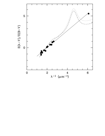
Figure 3: Normalized extinction $X(x)$ towards NGC 6565. The solid line is a linear fit to the data, $X(x)=-2.69+1.34x$. The dotted line and long-dashed lines are standard Galactic reddening law for $R_{\rm V}=3.1$ given by H83 and CCM89, respectively.

Table 4: Extinction towards individual nebulae.

Name	$c({\rm H}\beta)$				$R_{\rm V}$	$f(\lambda)^{d}$
	opt.	rad.	UV	adopt
Cn 1-5	0.49	0.39	0.59b	0.49	3.05	$-$0.91,0.44
Cn 2-1	1.07	0.83		0.83	3.10	CCM89
H 1-35	1.51	0.96		1.31	3.27	CCM89
H 1-41	0.65	0.67		0.65	3.45	$-$1.21,0.59
H 1-42	0.87	0.74		0.77	3.35	$-$1.31,0.64
H 1-50	0.68	0.53		0.68	3.70	$-$1.15,0.56
H 1-54	1.54	0.68		1.53	1.92	$-$2.26,1.09
He 2-118a	0.17	0.14		0.16	3.85
IC 4699	0.23	0.45	0.16	0.22	3.21	$-$1.42,0.69
IC 4846	0.69	0.34		0.65	2.79	CCM89
M 1-20	1.40	1.02		1.13	3.40	CCM89
M 1-29	2.03	1.63		1.83	3.10	CCM89
M 1-61	0.92	0.92		0.92	1.81	$-$2.31,1.12
M 2-4	1.33	0.81		0.81	1.97	CCM89
M 2-6	1.14	0.84		0.85	2.62	CCM89
M 2-23	1.20	0.98		1.12	2.97	CCM89
M 2-27	1.31	1.37		1.35	2.61	CCM89
M 2-31	1.41	1.18		1.15	3.07	CCM89
M 2-33	0.55	0.61		0.55	3.00	CCM89
M 2-39	0.61	0.63		0.63	1.92	CCM89
M 2-42	1.06	0.66		0.65	1.97	CCM89
M 3-7	1.65	1.51		1.46	4.18	H83
M 3-21	0.50	0.37	0.78	0.35	2.92	$-$1.27,0.62
M 3-29	0.24	0.12		0.12	1.86	CCM89
M 3-32	0.64	0.40	0.69	0.62	3.10	H83
M 3-33	0.50	0.42	0.32	0.39	3.31	CCM89
N 6439	1.10	0.93	1.15	0.93	2.81	CCM89
N 6565	0.32	0.36	0.52	0.37	3.10	$-$1.03,0.50
N 6567	0.90	0.66	0.73c	0.73	3.36	H83
N 6620	0.52	0.46	0.86	0.43	3.10	CCM89
Vy 2-1	0.83	0.66		0.64	2.80	CCM89

• Only a lower limit for the 5 GHz flux is available from the literature. Thus $c({\rm H}\beta)$ derived from the radio continuum to H$\beta$ flux ratio is an upper limit, as is $R_{\rm V}$.

• Derived from the He ii $\lambda$1640/$\lambda$3203 ratio.

• Derived from the UV continuum.

• Extinction law used to fit the extinction curve. H83 and CCM89 denote extinction laws given by (Howarth1983) and Cardelli et al. (1989), respectively. When two numbers are listed, it denotes a linear extinction law, $f(\lambda)=a+bx$, and the two numbers refer to values of $a$ and $b$, respectively. $x\equiv 1/\lambda(\mu{\rm m})$.

Excluding He 2-118, for which only a lower limit on its 5 GHz flux density is available from the literature, for the remaining 30 sample PNe, the normalized extinction, $X(x)$, was derived for each object at wavelengths of all usable lines. The logarithmic extinction, $f(\lambda)$, commonly used in nebular analyses and defined such that $f(\lambda)=0$ at H$\beta$, was also calculated. $f(\lambda)=0.4A(\lambda)/c({\rm H}\beta)-1$, where $c({\rm H}\beta)=0.4A({\rm H}\beta)$ is the logarithmic extinction at H$\beta$. The deduced normalized extinction curve was then compared with the H83 law and the CCM89 law. For eight sample nebulae, reliable fluxes of the He ii $\lambda$1640 line and/or the $\lambda$3203 line are available, providing an estimate of the extinction in the UV. For four of them, the extinction $X(x)$ shows a very good linear relation extending from optical to the UV. For the four objects, a linear function was used to fit $X(x)$ as a function of $x$. The resultant extinction curve was then used to deredden the observed line flux. For the other four PNe, either the H83 or the CCM89 law was used to fit the data, depending on which one yielded a better fit. We note that the two extinction laws have noticeable differences in the 3500–4500 Å wavelength range.

For the 22 remaining nebulae for which no estimate of UV extinction was possible, the extinction curve was either fitted with a linear function, the H83 law or the CCM89 law, whichever yielded the best fit. The extinction law used for each nebula is listed in the last column of Table 4. If an entry in this column consists of two numbers, it denotes a linear extinction law, $f(x)=a+bx$, was used, and the two numbers refer to fitted values of parameters $a$ and $b$, respectively. In Table 4, we also list values of $c({\rm H}\beta)$ derived from ratios of H$\alpha$/H$\beta$ (Column 2), $F_{\nu}$(5GHz)/H$\beta$ (Column 3) and of He ii $\lambda$1640/$\lambda$4686 (Column 4), as well as our final adopted values (Column 5) used to deredden the observed line fluxes. Finally, Column 6 of Table 4 gives the total-to-selective extinction ratio $R_{\rm V}$.

3.2 CEL plasma diagnostics

Table 5: Plasma diagnostic line ratios and ionization potentials of the emitting ions. Subscripts ’n’, ’a’ and ’f’ represent nebular, auroral and fine-structure lines, respectively.

ID		IP (eV)
	$T_{\rm e}$-diagnostics
[O ii]na	$I(\lambda 7320+\lambda 7330)/I(\lambda 3726+\lambda 3729)$	13.6
[N ii]na	$I(\lambda 6548+\lambda 6584)/I(\lambda 5754)$	14.5
[O iii]na	$I(\lambda 4959+\lambda 5007)/I(\lambda 4363)$	35.1
[Ne iii]nf	$I(15.5\mu{\rm m})/I(\lambda 3868)$	41.0
[Ar iii]nf	$I(9.0\mu{\rm m})/I(\lambda 7135)$	27.6
	$N_{\rm e}$-diagnostics
[S ii]nn	$I(\lambda 6731)/I(\lambda 6716)$	10.4
[O ii]nn	$I(\lambda 3729)/I(\lambda 3726)$	13.6
[Cl iii]nn	$I(\lambda 5537)/I(\lambda 5517)$	23.8
[Ar iv]nn	$I(\lambda 4740)/I(\lambda 4711)$	40.7
[Ne iii]ff	$I(15.5\mu{\rm m})/I(36.0\mu{\rm m})$	41.0

Table 6: Electron temperatures and densities from CELs. ‘H’ and ‘L’ denote the measured line ratio exceeds its high and low temperature/density limit, respectively, whereas ‘E’ indicates that recombination contribution as estimated using Eqs. (1) and (2) exceeds the actual measured flux of the [N II] $\lambda 5755$ line or of the [O II] $\lambda\lambda 7320,7330$ lines.

Nebula	$T_{\rm e}$(CELs) (K)				$N_{\rm e}$(CELs) (cm-3)
	[O iii]na	[N ii]na	[O ii]na		[O ii]nn	[S ii]nn	[Cl iii]nn	[Ar iv]nn
He 2-118	12630	14960	H		4.03	3.95	4.06	4.47
M 2-4	8570	9920	14570		3.72	3.82	3.83	3.98
M 2-6	10100	9730	11650			3.90	3.80	3.92
M 3-7	7670	6900	5110			3.74	3.43
M 1-20	9860	11180	16570		4.02	4.00	3.95	4.05
NGC 6439	10360	9270	11340		3.59	3.70	3.70	3.83
H 1-35	9060	12080	13720		4.45	4.69	4.54	L
M 1-29	10830	9020	9000			3.51	3.66	3.68
Cn 2-1	10250	12030	H		3.82	3.70	3.89	4.34
H 1-41	9800	9530	12790			3.11	3.07	2.96
H 1-42	9690	9050	13270			3.97	3.72	3.90
M 2-23	11980	H	H			4.23	4.08	4.76
M 3-21	9790	12800	19000		3.79	4.08	4.03	4.41
H 1-50	10950	12070	15360		3.83	3.87	3.96	4.15
M 2-27	11980	8650	8840			3.88	4.11	4.12
H 1-54	9540	11600	11360			4.11	4.12
NGC 6565	10300	10100	10200			3.25	3.19	2.82
M 2-31	9840	11370	13470			3.82	3.84	3.69
NGC 6567	10580	10016	14360		3.93	3.85	3.89	3.96
M 2-33	8040	9150	11070			3.21	L	3.14
IC 4699	11720	12490	9390			3.49	L	3.06
M 2-39	8050	8300	11030			3.68	3.17	3.38
M 2-42	8470	9350	11860			3.51	3.46	3.62
NGC 6620	9590	8630	9630		3.35	3.39	3.44	3.43
Vy 2-1	7860	8580	8750			3.51	3.69	3.52
Cn 1-5	8770	8250	10330			3.66	3.52	3.36
M 3-29	9190	8750	8930			2.91
M 3-32	8860	8230	E		3.55	3.41	2.94	3.13
M 1-61	8900	11510	8460			4.30	4.24	4.40
M 3-33	10380		7480			3.01	3.19	3.56
IC 4846	9930	13280	H			3.82	3.70	3.92

Accurate determinations of abundances rely on the reliable measurements of $T_{\rm e}$  and $N_{\rm e}$. In what follows, we present detailed plasma diagnostics using both CELs and recombination lines/continua. Values of $N_{\rm e}$  and $T_{\rm e}$, have been derived from CEL diagnostic ratios by solving equations of statistical equilibrium of multi-level ($\geq 5$) atomic models using equib, a Fortran code originally written by I. Howarth and S. Adams. CEL diagnostic lines used are tabulated in Table 5, together with the ionization potentials required to create the emitting ions. The atomic parameters used in the present work are the same as those used by Liu et al. (2000) in their case study of NGC 6153.

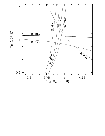
Figure 4: CEL plasma diagnostic diagram for NGC 6567. For diagnostic ID’s, c.f. Table 5.

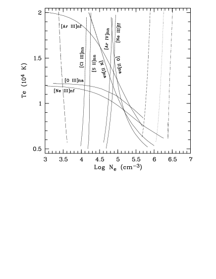
Figure 5: Plasma diagnostic diagram for M 2-23. For diagnostic ID’s, c.f. Table 5. The four broken lines represent density diagnostics from [Fe iii] lines (c.f. text for more details).

In order to obtain self-consistent results for $N_{\rm e}$  and $T_{\rm e}$  probed by CEL lines, we proceed as following. Firstly, $N_{\rm e}$([Cl iii]) and/or $N_{\rm e}$([Ar iv]) were obtained assuming a $T_{\rm e}$  of 10 000 K and then the average value of the derived $N_{\rm e}$  was adopted in calculating $T_{\rm e}$([O iii]). The calculations were iterated to obtain final self-consistent values of $N_{\rm e}$  and $T_{\rm e}$. We assume the results thus obtained represent physical conditions of the high ionization regions. Similarly, $T_{\rm e}$([N ii]) was derived in combination with $N_{\rm e}$([O ii]) and $N_{\rm e}$([S ii]) to represent the physical conditions in the low ionization zones. If all observed optical $N_{\rm e}$-indicators yielded similar values of $N_{\rm e}$, the results were averaged and used for the whole nebulae, both the high and low ionized regions. Recombination contributions to intensities of the [O ii] and [N ii] auroral lines were corrected for using the formulae derived by  Liu et al. (2000),

$$\frac{I_{\rm R}({\lambda 5755})}{I({\rm H}\beta)}=3.19t^{0.30}\times\frac{{\rm N}^{2+}}{{\rm H}^{+}},$$ (1)

$$\frac{I_{\rm R}({\lambda 7320+\lambda 7330})}{I({\rm H}\beta)}=9.36t^{0.44}\times\frac{{\rm O}^{2+}}{{\rm H}^{+}},$$ (2)

where ${\rm O}^{2+}$/${\rm H}^{+}$ and ${\rm N}^{2+}$/${\rm H}^{+}$ are ionic abundances derived from ORLs, and $t\equiv T_{\rm e}/10^{4}$K.

Wang et al. (2004) have examined the four optical $N_{\rm e}$-diagnostics, [O ii] $\lambda 3729/\lambda 3726$, [S ii] $\lambda 6716/\lambda 6731$, [Cl iii] $\lambda 5517/\lambda 5537$ and [Ar iv] $\lambda 4711/\lambda 4740$, for a sample of over 100 PNe, including 31 PNe in the current sample. The atomic parameters recommended in their work were adopted in the current study. For objects in common, $N_{\rm e}$  presented here differ by no more than 1 per cent from those published by Wang et al. (2004).

Fig. 4 and 5 present plasma diagnostic diagrams for NGC 6567 and M 2-23, respectively, as two examples. In the case of NGC 6567, various $N_{\rm e}$-diagnostic lines yield consistent values of $N_{\rm e}$, so a constant $N_{\rm e}$  has been adopted in calculating $T_{\rm e}$  from the [N ii$]_{\rm na}$ and [O iii$]_{\rm na}$ nebular to auroral diagnostic line ratios. The two $T_{\rm e}$’s thus obtained were then adopted in calculating CEL abundances for singly ionized species and for species of higher ionization degrees, respectively.

Electron temperatures and densities derived from various CEL diagnostics are tabulated in Table 6. In the Table, ‘H’ and ‘L’ denote the measured line ratio exceeds its high and low temperature/density limit, respectively, whereas ‘E’ indicates that recombination contribution as estimated using Eqs.(1) and (2) exceeds the actual measured flux of the [N II] $\lambda 5755$ line or of the [O II] $\lambda\lambda 7320,7330$ lines.

Kingsburgh & Barlow (1994, KB94 hereafter) have examined the relation between $T_{\rm e}$([O iii]) and $T_{\rm e}$([N ii]) for a sample of Galactic PNe. They found that the ratio of the former to the later increases with increasing $I$($\lambda$4686), the intensity of He ii $\lambda$4686,

$$\frac{T_{\rm e}(\mbox{[O\,{\sc iii}]})}{T_{\rm e}(\mbox{[N\,{\sc ii}]})}=(1.15\pm 0.06)+(0.0037\pm 0.0009)I(\lambda 4686){,}$$

with a correlation coefficient of 0.69. A similar analysis for GBPNe in the WL07 sample and GDPNe in the TLW sample (c.f. § 7) exhibits similar positive correlation, as shown in Fig. 6. A linear fit to the 45 points in the Figure yields:

$$\frac{T_{\rm e}(\mbox{[O\,{\sc iii}]})}{T_{\rm e}(\mbox{[N\,{\sc ii}]})}=(0.91\pm 0.02)+(0.0049\pm 0.0008)I(\lambda 4686){,}$$

with a correlation coefficient of 0.70, which is roughly in agreement with that obtained by (Kingsburgh & Barlow1994).

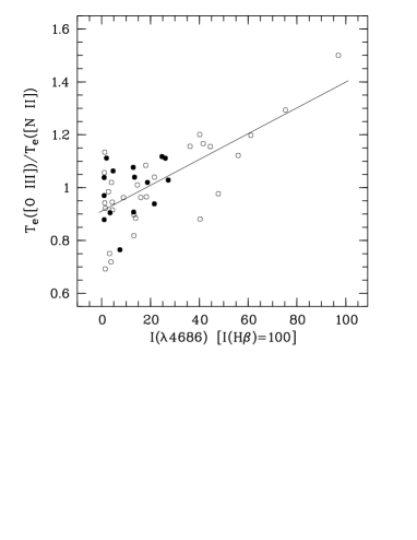
Figure 6: $T_{\rm e}$([O iii])/$T_{\rm e}$([N ii]) ratios against $I$($\lambda$4686) for GBPNe (filled circles) and GDPNe (open circles). The solid line is a linear fit to the 45 points in the Figure.

3.3 Two interesting objects

Table 7: Electron temperatures deduced from H i Balmer discontinuity, from He i recombination lines and from O ii ORLs, as well as electron density derived from the H i Balmer decrement. An ‘L’ denotes that the measured O ii $\lambda$4089/$\lambda$4649 exceeds its low temperature limit of 0.41 at 288 K.

Nebula	$T_{\rm e}$(H i) (K)	$T_{\rm e}$(He i) (K)				$T_{\rm e}$(O ii) (K)		$N_{\rm e}$(H i) (cm-3)
	BJ	$\frac{\lambda 6678}{\lambda 4471}$	$\frac{\lambda 5876}{\lambda 4471}$	$\frac{\lambda 7281}{\lambda 5876}$	$\frac{\lambda 7281}{\lambda 6678}$	$\frac{\lambda 4649}{\lambda 4089}$		BD
He 2-118	14500	12050	12870	5250	6800			5.0
M 2-4	7900		14100	6100	6100			4.6
M 2-6	11700	4300	2860	6200	6500	L
M 3-7	6900	8100	2580	1600	2500
M 1-20	12000			5100	6000			4.2
NGC 6439	9900	2060	1810	4810	4900	851		5.5
H 1-35	12000			5800	7300	334		4.8
M 1-29	10000	6900		4000	4100
Cn 2-1	10800	6750		5050	5450	857		5.0
H 1-41	4500	7110	5770	2690	2930	L
H 1-42	10000	3700	2250	5890	6290	662
M 2-23	5000	4900	1320	6100	7330	410
M 3-21	10400	3480	2150	5170	5520	602		5.0
H 1-50	12000	9050	3100	5420	6480	L		5.1
M 2-27	14000	8410		2280	2920
H 1-54	12500	13600	10400	4270	5840
NGC 6565	8500	3850	6400	4620	4090	11722
M 2-31	14000	2170	1220	3820	4460
NGC 6567	14000	7850	2670	6720	7790			4.0
M 2-33	7000	8510	5200	4050	4650	L
IC 4699	12000	7300	5950	3310	2460	L
M 2-39	5500	6810	7070	6610	6600	L
M 2-42	14000	8000	7700	3600	3300
NGC 6620	8200	2500	2400	3800	3800	3162		4.0
Vy 2-1	8700	5500	4550	4750	4970	L
Cn 1-5	10000	11600		2450	2940	18000
M 3-29	10700	6800	4750	1600	1800
M 3-32	4400	3860	3100	1560	1710	L		3.6
M 1-61	9500	18500		3500	5490
M 3-33	5900	6650	3940	4380	5020	1465
IC 4846	18000	6530	2430	6080	6970	9954

For most nebulae in our sample, diagnostics that sample respectively the high and the low ionized regions generally yield $N_{\rm e}$  of relatively small differences, as in the case of NGC 6567 (Fig. 4). There are however a few exceptions, such as M 2-23. For this object, as shown in Fig. 5, lines emitted by ions of high ionization potentials (i.e., [Ar iv]_nn and [Ne iii]_ff) yield a $N_{\rm e}$  of $\sim 10^{4.7}$ cm^-3, approximately 0.8 dex higher than derived from lines of low ionization potentials, such as [S ii]_nn. We note that for this nebula, the [N ii]_na and [O ii]_na nebular to auroral line ratios become sensitive to $N_{\rm e}$  as well as to $T_{\rm e}$. M 2-23 thus shares some similarities with Mz 3 and M 2-24, in that both have been previously found to harbour a dense emission core surrounded by an outer lobe of much lower densities (c.f. Zhang & Liu2002, Zhang & Liu2003). In (Zhang & Liu2002), high critical density [Fe iii] diagnostic lines were used to probe the physical conditions in the dense central emission core of Mz 3. The [Fe iii] line strengths observed in M 2-23 are on the average about a third of those detected in Mz 3. Unfortunately, lines sensitive to $T_{\rm e}$, such as the $\lambda$6096 or the $\lambda$7088 lines were all too faint to be detectable in our current spectra of M 2-23. In Fig. 5, we show, from left to right, the loci of four [Fe iii] $N_{\rm e}$-sensitive diagnostic line ratios, $\lambda 4659/\lambda 4770$, $\lambda 4755/\lambda 4881$, $\lambda 4770/\lambda 4778$ and $\lambda 4702/\lambda 4734$. Except for the first line ratio, which is less reliable given the intrinsic weakness of the [Fe iii] $\lambda 4770$ line, all the other three consistently yield a $N_{\rm e}$ $\sim\,$10⁶ cm^-3, comparable to the value of $\sim 10^{6.5}$ cm^-3 found for Mz 3 by (Zhang & Liu2002) and considerably higher than values given by other $N_{\rm e}$-diagnostics of lower critical densities.

In the ISO SWS spectrum of M 2-23, apart from the ionic fine-structure lines from heavy elements, H i Br$\alpha$, Br$\beta$ and Pf$\alpha$ lines were also well detected. The relative strengths of those high excitation H i recombination lines have a weak dependent on $T_{\rm e}$. Using the emission coefficients given by (Storey & Hummer1995), we determined a $T_{\rm e}$  of 5 000 K, with an uncertainty about 1 500 K. The value is very similar to that deduced from the H i Balmer discontinuity.

Another object in our sample that exhibits some interesting characteristics is M 2-39. For this nebula, all $N_{\rm e}$-diagnostic line ratios measurable in the optical, [S ii]_nn, [Cl iii]_nn and [Ar iv]_nn, consistently yield a low $N_{\rm e}$  between 1 500 and 5 100 cm^-3, whereas the [N ii]_na ratio gives a $T_{\rm e}$  of 8 300 K (Table 6). Yet the observed [O iii]_na ratio shows an abnormally low value of 25, indicating a $T_{\rm e}$  of about 28 000 K for a $N_{\rm e}$  of below 10 000 cm^-3. The [O iii]_na temperature could be lower if the density prevailing in the O²⁺ zone is much higher than 10 000 cm^-3. Some evidence in favour of a dense O²⁺ zone is provided by a well observed feature near 7171 Å, which we tentatively identified as the [Ar iv] $\lambda$7170.62 line. If the identification is correct, then its intensity relative to the [Ar iv] $\lambda\lambda$4711,4740 nebular lines would indicate a $N_{\rm e}$  of $10^{6.6}$ cm^-3. For comparison, if we assume a $T_{\rm e}$  of 10 000 K, as indicated by [N ii]_na and [O ii]_na, then a $N_{\rm e}$  as high as $10^{6.2}$ cm^-3 would be required to reproduce the measured [O iii]_na ratio. The identification of the feature at 7171 Å as [Ar iv] was however marred by the fact that another [Ar iv] line, at 7263 Å, expected to have a strength only 30 per cent lower than that of the [Ar iv] $\lambda$7171, was either absent or had at most a strength only one third of the measured strength of the 7171 Å feature. Clearly, better data are needed to clarify whether M 2-39 also contains a dense high excitation emission core as in the case of Mz 3, M 2-24 and probably also of M 2-23. In our current analysis, we have adopted a $N_{\rm e}$  of $10^{6.6}$ cm^-3 for the high ionization regions of M 2-39, assuming that the 7171 Å is indeed entirely due to [Ar iv]. Then the observed [O iii]_na ratio yields a $T_{\rm e}$  of 8 050 K (c.f. Table 6). This $N_{\rm e}$  and $T_{\rm e}$  have been used to calculate ionic abundances of heavy element ions from the high ionization regions. We note that the abundances thus obtained were abnormally high compared to other bugle PNe in the sample, even higher than values deduced from ORLs for the same object in the case of carbon and oxygen (c.f. Table 14). These abundances are however quite uncertain and should be treated with caution.

Given their peculiarities, both M 2-23 and M 2-39 will be excluded in our statistical analysis of the abundance patterns of GBPNe, leaving a sample size of 23.

3.4 Hydrogen recombination temperatures and densities

Electron temperatures have been determined for all sample PNe from the Balmer discontinuity of H i recombination spectra with various levels of uncertainty depending on the resolution and S/N ratios of spectra available for the wavelength range of the Balmer jump at 3650 Å. For practical reasons of measurement and following Liu et al. (2001), we define the Balmer jump, BJ, as the difference of continuum flux densities measured at 3643 and 3681 Å, i.e. $I_{\rm c}(\lambda 3643)-I_{\rm c}(\lambda 3681)$. Balmer jump temperature, $T_{\rm e}$(BJ), was then calculated from the ratio of Balmer jump to H 11 using the formula provided by Liu et al. (2001),

$$T_{\rm e}=368\times(1+0.259y^{+}+3.409y^{2+})(\frac{\rm BJ}{\rm H11})^{-\frac{3}{2}},$$ (3)

where BJ/H11 is in units of Å^-1 and $y^{+}$ and $y^{2+}$ denote helium ionic abundances, He⁺/H⁺ and He²⁺/H⁺, respectively. Since $y^{+}$ and $y^{2+}$ derived from helium recombination lines also have a weak dependence on adopted $T_{\rm e}$, the process was iterated until self-consistent values for $y^{+}$ and $y^{2+}$ and $T_{\rm e}$(BJ) were achieved. The results are tabulated in the second column of Table 7.

Electron densities, $N_{\rm e}$(BD)’s, were also derived by comparing the observed decrement of high-order Balmer lines with that predicted by recombination theory and are presented in the last column of Table 7.

(Zhang et al.2004) present determinations of $T_{\rm e}$(BJ) and $N_{\rm e}$(BD) for a sample of 48 Galactic PNe, including some objects in the current sample, by fitting the observed spectra with synthesized theoretical spectra with $T_{\rm e}$  and $N_{\rm e}$  as input parameters. The technique only works well for high resolution spectra. For objects in common, our current results are in good agreement with those presented in (Zhang et al.2004). For objects having high resolution spectra, typical uncertainties in $T_{\rm e}$(BJ) are about 1000 K. For those for which only low resolution spectra are available, the uncertainties increase to about 2000 K.

3.5 Helium temperatures

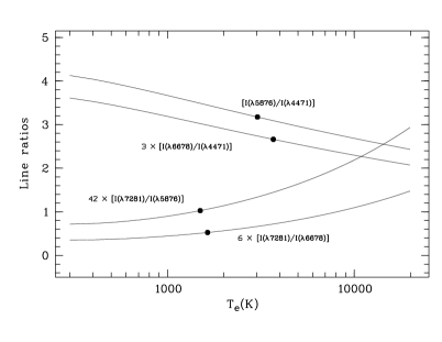
Figure 7: He i line ratios as a function of $T_{\rm e}$, assuming $N_{\rm e}$= 4000 cm^-3. The ratios observed in M 3-32 are marked.

Electron temperatures have been derived from He i recombination line ratios $\lambda 6678/\lambda 4471$, $\lambda 5876/\lambda 4471$, $\lambda 7281/\lambda 5876$, $\lambda 7281/\lambda 6678$ and are presented in Cols. 3–6 of Table 7. Albeit the lines involved are weaker, $T_{\rm e}$  determined from the fourth pair of diagnostic line ratio has a number of advantages over those deduced from the other three pairs (c.f. Zhang et al.2005 for details) and will be adopted in the current work. In Fig. 7, we show variations of the four He i line ratios as a function of $T_{\rm e}$  for an assumed $N_{\rm e}$ = 4000 cm^-3. Values measured in M 3-32 are marked as an example. The parameters used to calculate emissivities of He i lines are taken from Table 2 of (Zhang et al.2005). In their analysis, (Zhang et al.2005) presented He i temperatures deduced from the $\lambda 7281/\lambda 5876$ and $\lambda 7281/\lambda 6678$ ratios for a large sample of Galactic PNe; 9 of them are also in the current sample. For objects in common, $T_{\rm e}$  obtained by them are slightly higher than ours. The differences are mainly caused by the differences in extinction corrections. In their analysis, they had adopted the standard H83 extinction law for the general ISM and determined extinction to individual nebulae based on optical data alone. In the current work, a much more detailed and thorough treatment of the extinction has been carried out (c.f. Section 3.1).

3.6 Temperatures from heavy element ORLs

Liu et al. (2001) compared the observed relative intensities of O ii ORLs with predictions of the recombination theory in four PNe exhibiting particularly large adfs, M 1-42, M 2-36, NGC 7009 and NGC 6153. They found that while the agreement was quite good in general, there were exceptions. For example, the intensity of the strongest 3p-3s transition, 3p ⁴D${}^{\rm o}_{7/2}$ – 3s⁴P_5/2 $\lambda$4649, appears to be too strong (by $\sim 40$ per cent) relative to the strongest 4f – 3d transition, 4f G[5]${}^{\rm o}_{11/2}$ – 3d⁴F_9/2 $\lambda$4089, compared to the theoretical value calculated at $T_{\rm e}$ (BJ). It was later realized that the discrepancies were actually caused by the fact that those heavy element ORLs arise mainly from another component of plasma of very low $T_{\rm e}$, much lower than values deduced from the Balmer discontinuity of H i recombination spectrum (Liu 2003). By comparing observed ratios of the two strongest O ii  ORLs, $\lambda$4089/$\lambda$4649, with the theoretical predictions calculated down to a minimum $T_{\rm e}$  of 288 K, values of $T_{\rm e}$(O ii), the average $T_{\rm e}$  under which O ii ORLs are emitted, have been determined for a large sample of PNe (Tsamis et al.2004, Liu et al.2004b, Wesson et al.2005).

For the current sample of PNe, we have been able to determine $T_{\rm e}$(O ii) for 11 objects from the $\lambda$4089/$\lambda$4649 ratio. The results are presented in Col. 7 of Table 7. For another 8 nebulae in the sample (flagged with an ‘L’ in Table 7) for which both lines have been detected, the measured line ratios exceed 0.41, the maximum value at the low $T_{\rm e}$  limit of 288 K. Part of the discrepancy was clearly caused by measurement uncertainties, given the weakness of the lines. There is also an opportunity that the O ii $\lambda$4089.3 may have been contaminated by the Si iv $\lambda$4088.8 line, leading to artificially high $\lambda$4089/$\lambda$4649 ratios in some PNe (Liu 2006b; c.f. also Secction 6.1).

4 Ionic and total elemental abundances

4.1 Ionic abundances from CELs

Table 8: Ionic and elemental abundances of helium from ORLs. Ionic and elemental abundances of oxygen from CELs and from ORLs.

	He			CELs				ORLs
Nebula	He+/H+	He2+/H+	He/H	O+/H+	O2+/H+	$f$(O)	O/H	O2+/H+	$f$(O)	O/H
	average	$\lambda$4686		$\lambda\lambda$3726,29	$\lambda\lambda 4959,5007$			average
He 2-118	8.00e$-$02	8.00e$-$03	8.80e$-$02	7.91e$-$06	1.99e$-$04	1.065	2.20e$-$04	3.44e$-$04	1.108	3.81e$-$04
M 2-4	1.16e$-$01		1.16e$-$01	5.63e$-$05	4.76e$-$04	1.000	5.33e$-$04	8.99e$-$04	1.118	1.00e$-$03
M 2-6	1.01e$-$01		1.01e$-$01	6.28e$-$05	2.37e$-$04	1.000	3.00e$-$04	5.55e$-$04	1.264	7.02e$-$04
M 3-7	1.22e$-$01	1.50e$-$03	1.24e$-$01	2.54e$-$04	4.41e$-$04	1.008	7.00e$-$04	1.94e$-$03	1.588	3.08e$-$03
M 1-20	9.50e$-$02	4.00e$-$05	9.50e$-$02	2.30e$-$05	3.57e$-$04	1.000	3.80e$-$04	4.95e$-$04	1.064	5.27e$-$04
NGC 6439	1.12e$-$01	2.10e$-$02	1.33e$-$01	5.82e$-$05	3.96e$-$04	1.121	5.09e$-$04	2.44e$-$03	1.286	3.14e$-$03
H 1-35	1.02e$-$01	2.00e$-$04	1.02e$-$01	5.21e$-$05	2.78e$-$04	1.001	3.31e$-$04	5.71e$-$04	1.188	6.79e$-$04
M 1-29	1.12e$-$01	3.30e$-$02	1.45e$-$01	1.08e$-$04	3.83e$-$04	1.187	5.84e$-$04	1.13e$-$03	1.523	1.72e$-$03
Cn 2-1	1.11e$-$01	8.00e$-$03	1.19e$-$01	6.93e$-$06	4.79e$-$04	1.047	5.09e$-$04	1.40e$-$03	1.062	1.49e$-$03
H 1-41	8.10e$-$02	2.10e$-$02	1.02e$-$01	1.99e$-$05	3.48e$-$04	1.166	4.29e$-$04	1.78e$-$03	1.232	2.20e$-$03
H 1-42	1.09e$-$01	7.00e$-$04	1.10e$-$01	3.21e$-$05	4.19e$-$04	1.004	4.53e$-$04	9.64e$-$04	1.081	1.04e$-$03
M 2-23	1.12e$-$01		1.12e$-$01	5.67e$-$06	2.58e$-$04	1.000	2.64e$-$04	3.73e$-$04	1.021	3.81e$-$04
M 3-21	1.14e$-$01	6.40e$-$03	1.20e$-$01	1.37e$-$05	6.30e$-$04	1.037	6.68e$-$04	1.66e$-$03	1.059	1.76e$-$03
H 1-50	9.50e$-$02	1.10e$-$02	1.06e$-$01	1.86e$-$05	4.28e$-$04	1.075	4.80e$-$04	1.22e$-$03	1.122	1.37e$-$03
M 2-27	1.27e$-$01	8.00e$-$04	1.28e$-$01	5.33e$-$05	6.86e$-$04	1.004	7.42e$-$04	1.50e$-$03	1.082	1.62e$-$03
H 1-54	8.70e$-$02	3.00e$-$05	8.70e$-$02	5.43e$-$05	1.87e$-$04	1.000	2.42e$-$04	4.77e$-$04	1.290	6.15e$-$04
NGC 6565	9.90e$-$02	1.50e$-$02	1.14e$-$01	1.50e$-$04	3.83e$-$04	1.098	5.86e$-$04	6.47e$-$04	1.530	9.90e$-$04
M 2-31	1.14e$-$01		1.14e$-$01	1.94e$-$05	4.37e$-$04	1.000	4.57e$-$04
NGC 6567	1.02e$-$01	9.00e$-$04	1.03e$-$01	1.24e$-$05	2.76e$-$04	1.005	2.90e$-$04	6.04e$-$04	1.051	6.35e$-$04
M 2-33	1.05e$-$01		1.05e$-$01	2.03e$-$05	4.93e$-$04	1.000	5.13e$-$04	1.06e$-$03	1.041	1.10e$-$03
IC 4699	8.00e$-$02	1.80e$-$02	9.80e$-$02	5.10e$-$06	2.67e$-$04	1.144	3.11e$-$04	1.66e$-$03	1.166	1.94e$-$03
M 2-39	1.12e$-$01		1.12e$-$01	6.55e$-$05	2.58e$-$03	1.000	2.64e$-$03	9.14e$-$04	1.025	9.37e$-$04
M 2-42	1.07e$-$01	3.00e$-$04	1.07e$-$01	3.21e$-$05	5.27e$-$04	1.001	5.60e$-$04	1.10e$-$03	1.062	1.17e$-$03
NGC 6620	1.11e$-$01	2.10e$-$02	1.32e$-$01	1.82e$-$04	5.11e$-$04	1.122	7.78e$-$04	1.63e$-$03	1.521	2.48e$-$03
VY 2-1	1.29e$-$01	5.00e$-$04	1.30e$-$01	1.09e$-$04	5.50e$-$04	1.002	6.60e$-$04	1.11e$-$03	1.200	1.33e$-$03
Cn 1-5	1.25e$-$01	8.00e$-$04	1.26e$-$01	2.02e$-$04	4.89e$-$04	1.004	6.93e$-$04	7.94e$-$04	1.418	1.13e$-$03
M 3-29	1.00e$-$01		1.00e$-$01	5.88e$-$05	2.63e$-$04	1.000	3.22e$-$04	5.76e$-$04	1.223	7.05e$-$04
M 3-32	1.14e$-$01	1.05e$-$02	1.24e$-$01	2.58e$-$05	3.83e$-$04	1.060	4.34e$-$04	6.80e$-$03	1.131	7.70e$-$03
M 1-61	1.04e$-$01		1.04e$-$01	3.66e$-$05	4.85e$-$04	1.000	5.22e$-$04	9.49e$-$04	1.075	1.02e$-$03
M 3-33	8.80e$-$02	1.70e$-$02	1.05e$-$01	6.87e$-$06	3.43e$-$04	1.125	3.94e$-$04	2.25e$-$03	1.147	2.58e$-$03
IC 4846	7.90e$-$02	2.00e$-$04	7.92e$-$02	5.01e$-$06	3.83e$-$04	1.001	3.88e$-$04	5.91e$-$04	1.014	6.00e$-$04

Table 9: Ionic and elemental abundances of carbon from CELs and from ORLs.

	CELs					ORLs
Nebula	C2+/H+	C3+/H+	$f$(C)	C/H		C2+/H+	C3+/H+	$f$(C)	C/H
	$\lambda$1908	$\lambda 1550$				$\lambda 4267$	$\lambda\lambda$4187,4650
He 2-118						6.03e$-$05		1.108	6.68e$-$05
M 2-4						3.10e$-$04	6.98e$-$05	1.118	4.25e$-$04
M 2-6						8.22e$-$05		1.264	1.04e$-$04
M 3-7							5.81e$-$04
M 1-20						3.45e$-$04	1.71e$-$04	1.064	5.49e$-$04
NGC 6439	2.12e$-$04		1.286	2.73e$-$04		7.89e$-$04	1.98e$-$04	1.147	1.13e$-$03
H 1-35						1.32e$-$04	3.16e$-$04	1.187	5.32e$-$04
M 1-29						5.15e$-$04		1.523	7.84e$-$04
Cn 2-1						3.82e$-$04	4.92e$-$04	1.014	8.87e$-$04
H 1-41						3.11e$-$04		1.232	3.83e$-$04
H 1-42	5.76e$-$05		1.081	6.23e$-$05		1.03e$-$04	1.68e$-$04	1.076	2.92e$-$04
M 2-23	4.30e$-$05		1.021	4.40e$-$05		6.01e$-$05	1.30e$-$04	1.021	1.94e$-$04
M 3-21	1.22e$-$04		1.059	1.29e$-$04		3.40e$-$04	1.27e$-$04	1.021	4.77e$-$04
H 1-50	6.41e$-$05		1.122	7.20e$-$05		4.14e$-$04	6.49e$-$04	1.043	1.11e$-$03
M 2-27						8.19e$-$04		1.082	8.86e$-$04
H 1-54						8.70e$-$05	4.93e$-$04	1.289	7.48e$-$04
NGC 6565	1.98e$-$04		1.530	3.03e$-$04		3.27e$-$04	5.47e$-$05	1.392	5.32e$-$04
M 2-31						2.96e$-$04	3.38e$-$03	1.044	3.84e$-$03
NGC 6567	7.80e$-$04		1.051	8.20e$-$04		1.61e$-$03	7.00e$-$03	1.044	9.00e$-$03
M 2-33	3.94e$-$04		1.041	4.10e$-$04		1.91e$-$04	1.10e$-$04	1.041	3.13e$-$04
IC 4699	1.02e$-$04		1.166	1.19e$-$04		5.18e$-$04	6.82e$-$05	1.019	5.97e$-$04
M 2-39	6.09e$-$03		1.025	6.25e$-$03		4.07e$-$04	5.91e$-$04	1.025	1.02e$-$03
M 2-42						1.58e$-$04	5.94e$-$04	1.060	7.98e$-$04
NGC 6620	1.45e$-$04		1.521	2.21e$-$04		8.25e$-$04	8.44e$-$05	1.355	1.23e$-$03
VY 2-1	3.96e$-$04		1.200	4.75e$-$04		3.06e$-$04	1.08e$-$04	1.197	4.96e$-$04
Cn 1-5	1.05e$-$03	1.70e$-$04	1.412	1.72e$-$03		1.49e$-$03		1.418	2.10e$-$03
M 3-29						3.33e$-$04		1.223	4.08e$-$04
M 3-32	2.61e$-$04		1.131	2.95e$-$04		2.93e$-$03	2.30e$-$04	1.067	3.37e$-$03
M 1-61						3.91e$-$04	1.79e$-$04	1.075	6.13e$-$04
M 3-33	9.96e$-$05		1.147	1.14e$-$04		3.72e$-$04	2.62e$-$04	1.020	6.47e$-$04
IC 4846	1.43e$-$04		1.014	1.45e$-$04		1.11e$-$04	1.52e$-$04	1.013	2.66e$-$04

Table 10: Ionic and elemental abundances of nitrogen from CELs and from ORLs.

	CELs					ORLs
Nebula	N+/H+	N2+/H+	$f$(N)	N/H		N2+/H+	N3+/H+	$f$(N)	N/H
	$\lambda\lambda 6548,6584$	$\lambda$1750				average	$\lambda$4379
He 2-118	1.54e$-$06		27.85	4.29e$-$05		1.56e$-$04		1.108	1.73e$-$04
M 2-4	1.82e$-$05		9.464	1.72e$-$04		3.84e$-$04		1.118	4.29e$-$04
M 2-6	1.12e$-$05		4.782	5.36e$-$05
M 3-7	3.29e$-$05		2.759	9.08e$-$05		1.07e$-$03		1.588	1.70e$-$03
M 1-20	5.29e$-$06		16.51	8.74e$-$05		4.31e$-$04	8.58e$-$05	1.064	5.50e$-$04
NGC 6439	3.14e$-$05	3.38e$-$04	0.304	4.72e$-$04		6.92e$-$04	2.11e$-$04	0.092	9.67e$-$04
H 1-35	8.16e$-$06		6.346	5.18e$-$05		2.46e$-$04	1.06e$-$04	1.187	4.18e$-$04
M 1-29	7.34e$-$05		5.393	3.96e$-$04		6.82e$-$04	2.92e$-$04	1.227	1.20e$-$03
Cn 2-1	4.28e$-$06		73.43	3.14e$-$04		2.98e$-$04	4.92e$-$04	1.013	8.01e$-$04
H 1-41	3.50e$-$06		21.53	7.55e$-$05		6.62e$-$04	1.06e$-$04	1.048	8.05e$-$04
H 1-42	4.94e$-$06		14.12	6.98e$-$05		6.88e$-$04		1.081	7.44e$-$04
M 2-23	2.18e$-$06		46.57	1.02e$-$04		7.81e$-$04	6.05e$-$05	1.021	8.60e$-$04
M 3-21	8.25e$-$06	8.38e$-$05	0.420	1.27e$-$04		2.14e$-$04	8.99e$-$05	0.098	3.25e$-$04
H 1-50	7.62e$-$06		25.84	1.97e$-$04			8.92e$-$05
M 2-27	4.56e$-$05		13.91	6.34e$-$04		1.50e$-$03		1.082	1.62e$-$03
H 1-54	8.39e$-$06		4.450	3.73e$-$05		4.15e$-$04	1.22e$-$05	1.289	5.51e$-$04
NGC 6565	6.98e$-$05		3.895	2.72e$-$04		9.03e$-$04	3.87e$-$05	1.345	1.27e$-$03
M 2-31	9.61e$-$06		23.49	2.26e$-$04
NGC 6567	2.20e$-$06	3.51e$-$04	0.024	3.62e$-$04		3.59e$-$04	8.94e$-$06	0.006	3.70e$-$04
M 2-33	2.23e$-$06		25.25	5.63e$-$05		4.96e$-$04		1.041	5.16e$-$04
IC 4699	3.57e$-$07		60.98	2.18e$-$05		2.32e$-$04	1.05e$-$04	1.016	3.43e$-$04
M 2-39	1.18e$-$05		40.28	4.77e$-$04		7.84e$-$04		1.025	8.04e$-$04
M 2-42	1.03e$-$05		17.45	1.80e$-$04		4.39e$-$04		1.062	4.67e$-$04
NGC 6620	8.39e$-$05		4.278	3.59e$-$04		6.41e$-$04	1.47e$-$04	1.305	1.03e$-$03
Vy 2-1	2.68e$-$05	2.08e$-$04	1.002	2.36e$-$04		5.51e$-$04		1.200	6.61e$-$04
Cn 1-5	1.32e$-$04	7.29e$-$04a	1.004	8.65e$-$04		4.93e$-$03		1.418	6.99e$-$03
M 3-29	1.74e$-$05		5.468	9.50e$-$05
M 3-32	5.27e$-$06		16.83	8.87e$-$05		2.24e$-$03	3.04e$-$04	1.063	2.70e$-$03
M 1-61	8.97e$-$06		14.23	1.28e$-$04		4.70e$-$04	8.51e$-$05	1.075	5.97e$-$04
M 3-33	4.19e$-$07		57.27	2.40e$-$05			9.80e$-$05
IC 4846	1.58e$-$06		77.45	1.22e$-$04		1.25e$-$04		1.014	1.27e$-$04

• ^a Derived from the [N iii] 57$\mu$m infrared fine-structure line.

Table 11: Ionic and elemental abundances of neon from CELs and from ORLs. Ionic and elemental abundances of argon from CELs.

	CELs			ORLs		CELs
Nebula	Ne2+/H+	$f$(Ne)	Ne/H	Ne2+/H+	Ne/H	Ar2+/H+	Ar3+/H+	Ar4+/H+	$f$(Ar)	Ar/H
	$\lambda$3868			average		$\lambda$7136	$\lambda\lambda$4711,4740	$\lambda$7006
He 2-118	4.46e$-$05	1.108	4.94e$-$05	1.55e$-$03	1.72e$-$03	4.29e$-$07	7.64e$-$08		1.037	5.24e$-$07
M 2-4	1.22e$-$04	1.118	1.37e$-$04			2.56e$-$06	1.07e$-$07		1.118	2.98e$-$06
M 2-6	4.30e$-$05	1.264	5.44e$-$05			6.42e$-$07	3.10e$-$08		1.264	8.50e$-$07
M 3-7	6.77e$-$05	1.588	1.08e$-$04			6.33e$-$07			1.568	9.93e$-$07
M 1-20	6.04e$-$05	1.064	6.43e$-$05			5.87e$-$07	7.33e$-$08		1.064	7.03e$-$07
NGC 6439	1.26e$-$04	1.286	1.61e$-$04	1.35e$-$03	1.74e$-$03	2.27e$-$06	8.06e$-$07	1.01e$-$07	1.071	3.40e$-$06
H 1-35	3.50e$-$05	1.188	4.16e$-$05	8.57e$-$05	1.02e$-$04	1.35e$-$06	1.88e$-$08		1.187	1.63e$-$06
M 1-29	9.39e$-$05	1.523	1.43e$-$04			1.95e$-$06	8.96e$-$07		1.227	3.49e$-$06
Cn 2-1	9.46e$-$05	1.062	1.01e$-$04	4.99e$-$04	5.30e$-$04	1.24e$-$06	4.22e$-$07		1.013	1.68e$-$06
H 1-41	8.30e$-$05	1.232	1.02e$-$04			7.26e$-$07	4.27e$-$07		1.048	1.21e$-$06
H 1-42	8.56e$-$05	1.081	9.25e$-$05	1.24e$-$03	1.34e$-$03	9.03e$-$07	2.61e$-$07		1.076	1.25e$-$06
M 2-23	3.45e$-$05	1.021	3.52e$-$05	1.45e$-$04	1.48e$-$04	6.44e$-$07	7.62e$-$08		1.021	7.36e$-$07
M 3-21	1.72e$-$04	1.059	1.83e$-$04	8.65e$-$04	9.17e$-$04	1.81e$-$06	8.56e$-$07	4.80e$-$08	1.069	2.90e$-$06
H 1-50	1.10e$-$04	1.122	1.23e$-$04			9.87e$-$07	7.10e$-$07	5.69e$-$08	1.040	1.82e$-$06
M 2-27	1.90e$-$04	1.082	2.06e$-$04			3.08e$-$06	4.61e$-$07		1.077	3.81e$-$06
H 1-54	2.59e$-$05	1.290	3.34e$-$05	1.86e$-$04	2.40e$-$04	6.45e$-$07	1.17e$-$08		1.289	8.47e$-$07
NGC 6565	1.09e$-$04	1.530	1.67e$-$04	8.20e$-$04	1.26e$-$03	1.74e$-$06	4.04e$-$07	7.03e$-$08	1.345	2.99e$-$06
M 2-31	9.37e$-$05	1.044	9.79e$-$05			1.42e$-$06	3.68e$-$07		1.044	1.86e$-$06
NGC 6567	4.71e$-$05	1.051	4.94e$-$05	2.56e$-$04	2.69e$-$04	3.74e$-$07	1.20e$-$07		1.006	4.96e$-$07
M 2-33	9.88e$-$05	1.041	1.03e$-$04	7.04e$-$04	7.33e$-$04	1.20e$-$06	6.91e$-$08		1.041	1.32e$-$06
IC 4699	5.32e$-$05	1.166	6.20e$-$05	5.48e$-$04	6.39e$-$04	1.46e$-$06	4.10e$-$07		1.016	1.90e$-$06
M 2-39	2.10e$-$04	1.025	2.15e$-$04			3.01e$-$06	1.46e$-$06		1.025	4.58e$-$06
M 2-42	1.19e$-$04	1.062	1.27e$-$04			1.44e$-$06	1.59e$-$07		1.060	1.70e$-$06
NGC 6620	1.44e$-$04	1.521	2.19e$-$04	1.26e$-$03	1.92e$-$03	2.97e$-$06	6.23e$-$07	1.16e$-$07	1.305	4.84e$-$06
VY 2-1	1.41e$-$04	1.200	1.70e$-$04	4.04e$-$04	4.85e$-$04	2.41e$-$06	1.08e$-$07		1.128	2.84e$-$06
Cn 1-5	1.59e$-$04	1.418	2.26e$-$04	5.06e$-$04	7.18e$-$04	2.34e$-$06	7.19e$-$08		1.181	2.85e$-$06
M 3-29	5.81e$-$05	1.223	7.10e$-$05			6.33e$-$07			1.223	7.74e$-$07
M 3-32	1.13e$-$04	1.131	1.28e$-$04	2.00e$-$03	2.26e$-$03	1.31e$-$06	4.12e$-$07		1.063	1.83e$-$06
M 1-61	1.21e$-$04	1.075	1.31e$-$04	1.49e$-$03	1.60e$-$03	1.43e$-$06	1.06e$-$07		1.075	1.65e$-$06
M 3-33	8.87e$-$05	1.147	1.02e$-$04			6.17e$-$07	5.49e$-$07		1.017	1.19e$-$06
IC 4846	5.74e$-$05	1.014	5.83e$-$05			8.00e$-$07	2.29e$-$07		1.013	1.04e$-$06

Table 12: Ionic and elemental abundances of sulphur and chlorine from CELs.

	CELs					CELs
Nebula	S+/H+	S2+/H+	$f$(S)	S/H		Cl2+/H+	$f$(Cl)	Cl/H
	$\lambda\lambda$6716,6731	$\lambda 6312$				$\lambda\lambda 5517,5537$
He 2-118	1.11e$-$07	1.77e$-$07	2.127	6.13e$-$07		2.71e$-$08	3.461	9.37e$-$08
M 2-4	5.87e$-$07	1.92e$-$05	1.520	3.00e$-$05		1.69e$-$07	1.566	2.65e$-$07
M 2-6	2.76e$-$07	3.29e$-$06	1.255	4.48e$-$06		6.35e$-$08	1.360	8.64e$-$08
M 3-7	7.24e$-$07	8.09e$-$06	1.105	9.74e$-$06		1.64e$-$07	1.204	1.98e$-$07
M 1-20	1.68e$-$07	2.48e$-$06	1.802	4.77e$-$06		4.46e$-$08	1.924	8.58e$-$08
NGC 6439	1.12e$-$06	6.14e$-$06	1.485	1.08e$-$05		1.28e$-$07	1.755	2.25e$-$07
H 1-35	2.46e$-$07	6.94e$-$06	1.354	9.74e$-$06		9.25e$-$08	1.402	1.30e$-$07
M 1-29	2.39e$-$06	6.64e$-$06	1.295	1.17e$-$05		1.15e$-$07	1.762	2.03e$-$07
Cn 2-1	1.80e$-$07	4.18e$-$06	2.916	1.27e$-$05		6.95e$-$08	3.042	2.11e$-$07
H 1-41	1.43e$-$07	2.67e$-$06	1.959	5.52e$-$06		6.76e$-$08	2.064	1.40e$-$07
H 1-42	2.90e$-$07	3.53e$-$06	1.716	6.57e$-$06		8.18e$-$08	1.857	1.52e$-$07
M 2-23	1.16e$-$07	2.40e$-$06	2.512	6.33e$-$06		7.82e$-$08	2.633	2.06e$-$07
M 3-21	3.29e$-$07	6.00e$-$06	2.551	1.62e$-$05		1.22e$-$07	2.691	3.27e$-$07
H 1-50	3.57e$-$07	3.51e$-$06	2.076	8.02e$-$06		7.26e$-$08	2.288	1.66e$-$07
M 2-27	1.04e$-$06	1.04e$-$05	1.708	1.95e$-$05		2.01e$-$07	1.879	3.78e$-$07
H 1-54	1.93e$-$07	4.00e$-$06	1.232	5.17e$-$06		6.62e$-$08	1.292	8.55e$-$08
NGC 6565	2.52e$-$06	7.01e$-$06	1.192	1.14e$-$05		1.12e$-$07	1.622	1.81e$-$07
M 2-31	5.02e$-$07	6.05e$-$06	2.014	1.32e$-$05		1.01e$-$07	2.181	2.21e$-$07
NGC 6567	7.89e$-$08	1.36e$-$06	2.012	2.90e$-$06		3.48e$-$08	2.129	7.40e$-$08
M 2-33	5.95e$-$08	4.70e$-$06	2.061	9.80e$-$06		1.03e$-$07	2.087	2.15e$-$07
IC 4699	3.02e$-$08	7.59e$-$07	2.744	2.16e$-$06		3.96e$-$08	2.853	1.13e$-$07
M 2-39	3.81e$-$07	4.69e$-$06	2.396	1.21e$-$05		4.43e$-$06	2.591	1.15e$-$05
M 2-42	4.96e$-$07	6.46e$-$06	1.833	1.28e$-$05		1.35e$-$07	1.974	2.70e$-$07
NGC 6620	3.25e$-$06	9.40e$-$06	1.220	1.54e$-$05		1.82e$-$07	1.641	2.98e$-$07
VY 2-1	8.88e$-$07	1.00e$-$05	1.339	1.46e$-$05		1.53e$-$07	1.457	2.23e$-$07
Cn 1-5	2.55e$-$06	8.35e$-$06	1.158	1.26e$-$05		1.59e$-$07	1.511	2.40e$-$07
M 3-29	3.30e$-$07	3.48e$-$06	1.300	4.96e$-$06		8.38e$-$08	1.423	1.19e$-$07
M 3-32	2.46e$-$07	3.23e$-$06	1.813	6.29e$-$06		8.09e$-$08	1.951	1.58e$-$07
M 1-61	2.82e$-$07	2.65e$-$06	1.720	5.04e$-$06		9.30e$-$08	1.904	1.77e$-$07
M 3-33	1.93e$-$08	1.21e$-$06	2.688	3.30e$-$06		4.30e$-$08	2.731	1.17e$-$07
IC 4846	1.09e$-$07	3.36e$-$06	2.968	1.03e$-$05		7.09e$-$08	3.064	2.17e$-$07

Table 13: Ionization correction factors (ICFs).

X	Lines	Detected ions			X/H	Correction factors
C	ORLs & CELs		C2+	C3+	ICF$\times$($\frac{{\rm C}^{2+}}{{\rm H}^{+}}$ + $\frac{{\rm C}^{3+}}{{\rm H}^{+}}$)	$(\frac{{\rm O}^{+}+{\rm O}^{2+}}{{\rm O}^{2+}})_{\rm CELs}$
			C2+		ICF$\times(\frac{{\rm C}^{2+}}{{\rm H}^{+}})$	$(\frac{{\rm O}}{{\rm O}^{2+}})_{\rm CELs}$
N	CELs	N+	N2+		$(1+f_{1})\times\frac{{\rm N}^{2+}}{{\rm H}^{+}}+\frac{{\rm N}^{+}}{{\rm H}^{+}}$	$f_{1}=(\frac{{\rm N}^{3+}}{{\rm N}^{2+}})_{\rm ORLs}$
		N+	N2+		ICF$\times(\frac{{\rm N}^{2+}}{{\rm H}^{+}}+\frac{{\rm N}^{+}}{{\rm H}^{+}})$	$(\frac{{\rm He}^{+}+{\rm He}^{2+}}{{\rm He}^{+}})^{2/3}$
		N+			ICF$\times(\frac{{\rm N}^{+}}{{\rm H}^{+}})$	$(\frac{{\rm O}}{{\rm O}^{+}})_{\rm CELs}$
	ORLs		N2+	N3+	$(1+f_{2})\times\frac{{\rm N}^{2+}}{{\rm H}^{+}}+\frac{{\rm N}^{3+}}{{\rm H}^{+}}$	$f_{2}=(\frac{{\rm N}^{+}}{{\rm N}^{2+}})_{\rm CELs}$
			N2+	N3+	ICF$\times(\frac{{\rm N}^{2+}}{{\rm H}^{+}}+\frac{{\rm N}^{3+}}{{\rm H}^{+}})$	$[1-(\frac{{\rm O}^{+}}{{\rm O}})_{\rm CELs}]^{-1}$
			N2+		ICF$\times(\frac{{\rm N}^{2+}}{{\rm H}^{+}})$	$(\frac{{\rm O}}{{\rm O}^{2+}})_{\rm CELs}$
O	CELs	O+	O2+		ICF$\times(\frac{{\rm O}^{+}}{{\rm H}^{+}}+\frac{{\rm O}^{2+}}{{\rm H}^{+}})$	$(\frac{{\rm He}^{+}+{\rm He}^{2+}}{{\rm He}^{+}})^{2/3}$
	ORLs		O2+		ICF$\times\frac{{\rm O}^{2+}}{{\rm H}^{+}}$	$(\frac{{\rm He}^{+}+{\rm He}^{2+}}{{\rm He}^{+}})^{2/3}\times[1+(\frac{{\rm O}^{+}}{{\rm O}^{2+}})_{\rm CELs}]$
Ne	ORLs & CELs		Ne2+		ICF$\times\frac{{\rm Ne}^{2+}}{{\rm H}^{+}}$	$(\frac{{\rm O}}{{\rm O}^{2+}})_{\rm CELs}$
S	CELs	S+	S2+		ICF$\times(\frac{{\rm S}^{+}}{{\rm H}^{+}}+\frac{{\rm S}^{2+}}{{\rm H}^{+}})$	$[1-(1-\frac{{\rm O}^{+}}{{\rm O}})^{3}]_{\rm CELs}^{-1/3}$
Ar	CELs	Ar2+	Ar3+	Ar4+	ICF$\times(\frac{{\rm Ar}^{2+}}{{\rm H}^{+}}+\frac{{\rm Ar}^{3+}}{{\rm H}^{+}}+\frac{{\rm Ar}^{4+}}{{\rm H}^{+}})$	$[1-(\frac{{\rm N}^{+}}{{\rm N}})_{\rm CELs}]^{-1}$
		Ar2+	Ar3+		ICF$\times(\frac{{\rm Ar}^{2+}}{{\rm H}^{+}}+\frac{{\rm Ar}^{3+}}{{\rm H}^{+}})$	$[1-(\frac{{\rm N}^{+}}{{\rm N}})_{\rm CELs}]^{-1}$
Cl	CELs		Cl2+		ICF$\times\frac{{\rm Cl}^{2+}}{{\rm H}^{+}}$	$(\frac{{\rm S}}{{\rm S}^{2+}})_{\rm CELs}$

Abundances for ionic species of C, N, O, Ne, S, Ar, Cl and Fe have been determined from CELs for 31 sample nebulae. In the calculations, we have adopted $T_{\rm e}$ derived from [N ii]_na nebular to auroral line ratio and $N_{\rm e}$ derived from the [S ii]_nn nebular line ratio (or the average of values derived from the [S ii]_nn and [O ii]_nn ratios if the latter is available). For ionic species of higher ionization stages, $T_{\rm e}$  deduced from the [O iii]_na ratio and the average $N_{\rm e}$  derived from the [Cl iii]_nn and [Ar iv]_nn ratios were used. Note that for most objects, we have corrected for a recombination contribution to the [N ii] $\lambda$5755 auroral line, except for a few cases where the contamination as estimated using the aforementioned formula (and adopting an ionic abundance N²⁺/H⁺ as yielded by N ii ORLs) was found to be unphysically large, becoming comparable to or even larger than the actually measured total flux of the $\lambda$5755 feature. In the case of M 3-33, the [N ii] $\lambda$5755 line was too faint to have a reliable measurement. For this nebula $T_{\rm e}$[O iii] has been used to calculate abundances of all ionic species.

Ionic abundance ratios, ${\rm X}^{\rm i+}/{\rm H}^{+}$, derived from collisionally excited UV, optical and IR lines are tabulated in Tables 8 (oxygen), 9 (carbon), 10 (nitrogen), 11 (neon and argon) and 12 (sulfur and chlorine).

4.2 Ionic abundances from ORLs

4.2.1 He

Singly and doubly ionized helium abundances were derived from the He i $\lambda$4471, $\lambda$5876 and $\lambda$6678 recombination lines and from the He ii $\lambda$4686 recombination line, respectively. The results from the three He i lines were averaged, weighted by 1:3:1. The total helium abundances relative to hydrogen were obtained by summing abundances of singly and doubly ionized species. The results are tabulated in Cols. 2–4 of Table 8.

4.2.2 C, N, O, Ne and Mg

Ionic and elemental abundances have been derived from ORLs for some or all of the elements C, N, O, Ne and Mg for our sample of 31 PNe. Electron temperatures derived from the H i Balmer discontinuity, $T_{\rm e}$(BJ), were adopted in the calculations. For the 11 PNe of sub-sample A, $N_{\rm e}$(BD) were derivable and were adopted. For the remaining 20 PNe, the average $N_{\rm e}$  derived from various optical CEL diagnostics were used. For individual ionic species, we adopt the same effective recombination coefficients and assume the same case [Case A and B] as Liu et al. (2000), except for low $l$ transitions of N ii, for which the more recent calculations of Kisielius & Storey (2002) are used. For ionic species for which a host of lines have been detected, such as N ii, O ii and Ne ii, the results derived from individual transitions were averaged, according to procedures outlined in Liu et al. (1995) and Liu et al. (2000). The results are tabulated in Tables 8, 9, 10 and 11.

4.3 Elemental abundances

Table 14: Total elemental abundances on a logarithmic scale where H = 12.

Nebula	He	C		N		O		Ne		S	Cl	Ar	Mg
	ORLs	CELs	ORLs	CELs	ORLs	CELs	ORLs	CELs	ORLs	CELs	CEl	CELs	ORLs
Bulge PNe
M 2-4	11.06		8.63	8.24	8.63	8.73	9.00	8.14		7.48	5.42	6.47	7.70
M 2-6	11.00		8.02	7.73		8.48	8.85	7.74		6.65	4.94	5.93
M 3-7	11.09		8.96	7.96	9.23	8.85	9.49	8.03		6.99	5.30	6.00
M 1-20	10.98		8.74	7.94	8.74	8.58	8.72	7.81		6.68	4.93	5.85
NGC 6439	11.12	8.44	9.05	8.67	8.99	8.71	9.50	8.21	9.24	7.03	5.35	6.53
Cn 2-1	11.08		8.95	8.50	8.90	8.71	9.17	8.00	8.72	7.10	5.33	6.23
H 1-41	11.01		8.58	7.88	8.91	8.63	9.34	8.01		6.74	5.14	6.08
H 1-42	11.04	7.79	8.46	7.84	8.87	8.66	9.02	7.97	9.13	6.82	5.18	6.10
M 2-23a	11.05	7.64	8.29	8.01	8.93	8.42	8.58	7.55	8.17	6.80	5.31	5.87
M 3-21	11.08	8.11	8.68	8.10	8.51	8.82	9.25	8.26	8.96	7.21	5.51	6.45	7.53
H 1-50	11.03		9.05	8.29		8.68	9.14	8.09		6.90	5.22	6.26
M 2-27	11.11		8.95	8.80	9.21	8.87	9.21	8.31		7.29	5.58	6.58
H 1-54	10.94		8.87	7.57	8.74	8.38	8.79	7.52	8.38	6.71	4.93	5.93
NGC 6565	11.06	8.48	8.73	8.43	9.10	8.77	9.00	8.22	9.10	7.06	5.26	6.48	7.68
M 2-31	11.06		9.58	8.35		8.66		7.99		7.12	5.34	6.27
M 2-33	11.02	8.61	8.50	7.75	8.71	8.71	9.04	8.01	8.87	6.99	5.33	6.12
IC 4699	10.99	8.08	8.78	7.34	8.53	8.49	9.29	7.79	8.81	6.34	5.05	6.28	7.86
M 2-39a	11.05	9.80	9.01	8.68	8.91	9.42	8.97	8.33		7.08	7.06e	6.66
M 2-42	11.03		8.90	8.26	8.67	8.75	9.07	8.10		7.11	5.43	6.23
NGC 6620	11.12	8.34	9.09	8.56	9.01	8.89	9.39	8.34	9.28	7.19	5.47	6.69
Vy 2-1	11.11	8.68	8.70	8.37	8.82	8.82	9.12	8.23	8.69	7.17	5.35	6.45
Cn 1-5	11.10	9.24	9.32	8.94	9.84	8.84	9.05	8.35	8.86	7.10	5.38	6.45	7.37
M 3-29	11.00		8.61	7.98		8.51	8.85	7.85		6.70	5.08	5.89
M 3-32	11.10	8.47	9.53	7.95	9.43	8.64	9.89	8.11	9.35	6.80	5.20	6.26	7.93
M 3-33	11.02	8.06	8.81	7.38		8.59	9.41	8.01		6.52	5.07	6.07
Disk PNe
He 2-118	10.94		7.80	7.63	8.24	8.34	8.58	7.69	9.23	5.79	4.97	5.72
H 1-35	11.01		8.73	7.71	8.62	8.52	8.83	7.62	8.01	6.99	5.11	6.21
M 1-29	11.16		8.89	8.60	9.08	8.77	9.24	8.16		7.07	5.31	6.54
NGC 6567	11.01	8.91	9.95	8.56	8.57	8.46	8.80	7.69	8.43	6.46	4.87	5.70	7.80
M 1-61	11.02		8.79	8.11	8.78	8.72	9.01	8.12	9.20	6.70	5.25	6.22
IC 4846	10.90	8.16	8.43	8.09	8.10	8.59	8.78	7.77		7.01	5.34	6.02
Averageb	11.05	8.57	8.99	8.32	9.09	8.71	9.26	8.09	9.03	7.02	5.29	6.31	7.72
$\sigma$	0.05	0.18	0.86	0.15	0.17	0.13	0.54	0.20	0.30	0.30	0.19	0.27	0.21
Averagec	11.06	8.56	9.03	8.34	9.14	8.70	9.32	8.13	9.07	7.05	5.29	6.34	7.71
$\sigma$	0.05	0.18	0.86	0.15	0.17	0.13	0.54	0.20	0.30	0.30	0.19	0.27	0.21
Selected bulge samples from the recent literature
RPDM97	11.08			8.50		8.72		7.99		7.00	5.70	6.58
CMKAS00	10.98			8.29		8.74				6.92	5.10	6.35
EC01	11.09			7.84		8.47				6.98		6.32
ECM04	11.04			8.40		8.65		8.13		6.89		6.73
EBW04	11.05			8.43		8.66		8.03		7.05		6.60
Selected disk samples from the recent literature
KB94	11.06	8.74		8.35		8.68		8.09		6.92		6.39
TLWd	11.02	8.52	9.09	8.17	8.94	8.60	9.22	7.99	9.06	6.84	5.35	6.20	7.56
Solare	10.90	8.39		7.83		8.69		7.87		7.19	5.26	6.55	7.55

• ^a Excluded from statistical analyses (c.f. Section 3.3).

• ^b Average abundances for 23 GBPNe of the current sample.

• ^c Average abundances for 23 GBPNe of the current sample plus M 1-42 and M 2-36 previously analyzed by Liu et al. (2001).

• ^d Combined sample of 58 GDPNe (c.f. Section 7).

• ^e Lodders (2003).

Total elemental abundances were derived from ionic abundances (both from CELs and ORLs) using the same procedures and ionization correction factors (ICFs) adopted in (Wesson et al.2005). They are tabulated in Table 13. Ionic and elemental abundances as well as ICFs for individual elements, $f$(X), of all PNe are presented in Tables 8, 9, 10, 11 and 12.

No [Fe iv] lines have been detected in any of the nebulae and no ICF formula is available to obtain Fe/H elemental abundance from the Fe²⁺/H⁺ ionic abundance alone. As such, we have excluded Fe in our analysis. The Mg ii $\lambda 4481$ ORL has been detected in seven nebulae. Following Barlow et al. (2003), we assumed that the Mg ii $\lambda 4481$ has an effective recombination coefficient equal to that of the C ii $\lambda 4267$ line in calculating Mg²⁺/H⁺ from the observed strength of the $\lambda 4481$ line. In addition, considering the unusually wide ionization potential interval occupied by Mg²⁺, we assumed that Mg/H = Mg²⁺/H⁺, i.e. no need of applying any ICF corrections. As a consequence, no Mg²⁺/H⁺ ionic abundances are tabulated separately. Instead, only the total elemental abundances of magnesium are given in Table 14 (see below).

Total elemental abundances deduced for each nebula are presented in Table 14. For ease of comparison, we list abundances derived from both CELs and ORLs in the same Table. Also tabulated in the Table are average abundances of individual elements derived from the current sample of GBPNe, from other samples of GBPNe published in the literature, from the TLW (c.f. Section 7) and KB94 sample of GDPNe, as well as the solar photospheric abundances. Note that average abundances listed in the Table are logarithmic abundance averages (in units where H = 12), not averages of logarithmic abundances.

4.4 Abundance uncertainties

There are two major sources of uncertainty that affecting the derived element abundances: those propagating from line flux measurements and those arising from the analyzing methodology (e.g. those introduced via the application of empirical ICFs). Another potential source of error affecting in particular the current sample of objects is the uncertainty in the extinction law towards the Galactic center. The latter is difficult to characterize due to the lack of other independent means of measuring the extinction curve towards the Galactic center.

Uncertainties in line fluxes will also affect abundance determinations via derivations of $T_{\rm e}$  and $N_{\rm e}$. For most of our objects, we expect that flux measurements of strong lines (strengths larger than 0.008 relative to H$\beta$) should be accurate to better than 5 per cent. This encompasses essentially all diagnostic CELs, including the relatively weak [O iii] $\lambda 4363$ and [N ii] $\lambda 5755$ auroral lines, important for $T_{\rm e}$  determinations. We estimated that uncertainties in plasma diagnostics of CELs should typically be no more than 4 per cent in $T_{\rm e}$  and 30 per cent in $N_{\rm e}$, and their total effect on deduced ionic abundances should be less than 6 per cent. There are a few exceptions where the abundances were based on low critical density far-IR fine-structure lines, which are more sensitive to $N_{\rm e}$  variations.

Emissivities of ORLs have only a weak dependence on $T_{\rm e}$  and $N_{\rm e}$. However, those lines are generally much weaker than CELs and are often affected by serious line blending. For a few objects lacking high S/N, high resolution spectra, such as M 1-29, uncertainties in the derived ORL abundances of N, O and Ne could be as large as 30 per cent. The situation is much better for carbon, which has a few relatively strong well observed ORLs in the optical. Thus in most cases, we expect carbon abundances derived from ORLs to be accurate to better than 5 per cent. Comparable or even better accuracies are expected for helium abundances.

Alexander & Balick (1997) have investigated potential errors in abundance determinations that may result from applying the KB94’s ICF scheme when only optical lines are observed, by constructing a series of constant-density PN models. They found that the errors are smaller for small unresolved nebulae, and typically amount to $\la 10$ per cent for helium and oxygen, $\la 25$ per cent for nitrogen, sulfur and neon, but the abundances of argon are probably systematically overestimated. Given the large distance to the Galactic bulge, most PNe in our sample are quite compact, less than 10″  in diameter. A few objects in our sample have UV and/or IR spectra available. For those objects, we expect a better accuracy for nitrogen abundances.

In summary, we estimate that the total error budgets of our current abundance determinations are: 0.12 dex for He/H from ORLs and O/H from CELs, 0.26 to 0.30 dex for N/H, S/H, Ne/H, Ar/H and Cl/H from CELs, 0.12 dex for C/H from ORLs, 0.25 to 0.29 dex for O/H, N/H and Ne/H from ORLs.

5 Comparisons with previous studies

Hitherto several spectroscopic studies presenting approximately 350 abundance determinations for more than 250 GBPNe have been published. In this section, we will compare our results with those from some of the most recent ones, including W88 (Webster, 1988), RPDM97 (, Ratag et al.1997), SRM98  (Stasińska et al., 1998), CMKAS00 (, Cuisinier et al.2000), EC01  (Escudero & Costa, 2001), ECM04 (Escudero et al., 2004) and EBW04  (Exter et al., 2004). We will compare the general patterns of abundance obtained in Section 5.1 as well as individual measurements for common objects in Section 5.2. Unless otherwise specified, the current sample of 25 GBPNe, WL07, refers to the 23 GBPNe presented in the current paper (c.f. the first part of Table 14, with two peculiar objects, M 2-23 and M 2-39 excluded) plus M 1-42 and M 2-36 previously analyzed by Liu et al. (2001).

Except for Liu et al. (2001) presenting heavy element abundances deduced both from CELs and from ORLs for two GBPNe, essentially all abundance determinations of heavy elements for GBPNe published in the literature have been based on strong CELs only. Thus, comparisons will only be made for abundances derived from CELs. Also, carbon abundances have previously been measured only for a very small number of GBPNe, so the comparisons will concentrate on helium, oxygen, nitrogen and neon.

Note that much of the earlier work on GBPNe used the standard extinction law of the general diffuse ISM, which is known to be inapplicable for the Galactic centre (e.g. Udalski2003; Ruffle et al.2004), in particular in the UV. However, for analyses based on optical or infrared observations only, the uncertainties thus introduced were likely to be small. The recombination contribution to the [N ii] $\lambda$5755 auroral line was also uncorrected, leading to overestimated $T_{\rm e}$([N ii]) and consequently underestimated N⁺/H⁺, O⁺/H⁺ and S⁺/H⁺ ionic abundance ratios in some nebulae.

5.1 Comparisons of general patterns of abundances

W88 presented elemental abundances for a sample of 49 GBPNe, amongst which five are in common with our sample: M 2-27, M 2-33, M 3-7, M 3-33 and Cn 2-1. Her sample yields an average oxygen abundance of 8.73, very similar to the value of 8.70 deduced from the current sample (c.f. Table 14). For helium, her sample yields an average abundance of 11.06 (11.05 for non-Type I PNe), identical to the value deduced from the current sample. Note however, collisional excitation of He i was not corrected for in W88 – the effects typically amount to a few per cent. She did not present nitrogen abundances separately. From the N/O abundance ratios listed in her paper, we derive an average N/O ratio of $0.24$, much less than the average value of 0.40 deduced from the current sample, suggesting that nitrogen abundances obtained by W88 are systematically lower than ours by almost a factor of two.

RPDM97 presented abundances for a sample of about 110 GBPNe, deduced from their own observations or from line fluxes published in the literature. They used a grid of photoionization models to estimate ICFs, which were then used to calculate elemental abundances from abundances of observed ionic species. The average abundances calculated from values of individual nebulae presented in Table 5 of RPDM97 are listed in Table 14. For He, O and S, their results are in excellent agreement with ours (within 0.05 dex). For N, Cl and Ar, the differences are somewhat larger. For Cl and Ar, measurement uncertainties may play a role – weak lines of [Cl iii] and [Ar iv] might not be well measured in their low-resolution spectra. For nitrogen, parts of the discrepancy may arise from uncertainties in ICFs. For CEL abundance analyses, only the trace ionic species N⁺ is seen in the optical wavelength range. More abundant N⁺⁺ is only observable in the UV or the far infrared. Thus ICF corrections for nitrogen are often quite large and uncertain when only optical data are available.

SRM98 combined spectroscopic data published by (Aller & Keyes1987), W88 and RPDM97 and selected 90 objects with a 6 cm radio flux density less than 100 mJy, considered to belong to the Bulge population at the 90–95 per cent confidence level. They used an empirical abundance determination scheme similar to our CEL analyses and adopted the same set of ICFs given by KB94. However, they applied $T_{\rm e}$ derived from either the [O iii]_na or the [N ii]_na ratios for all ionic species in abundance calculations. For their GBPNe sample containing 85 objects with oxygen abundance measured, they derived a mean oxygen abundance 8.48 with a standard deviation ($\sigma$) of 0.434. For 32 brighter objects in their sample, the average abundance is 8.67 ($\sigma=0.213$). The latter is in good agreement with our result (c.f. Table 14).

CMKAS00 presented spectrophotometric observations and determined element abundances for a sample of 30 GBPNe. $T_{\rm e}$’s derived from the [N ii]_na and [O iii]_na ratios were adopted for low- and high-ionization zones, respectively, and $N_{\rm e}$’s were derived from the [S ii]_nn ratio. They used ICFs given by (Köppen et al.1991), which are the same as ours for He, N and Ne. Mean abundances of He, O, N, S, Cl and Ar, calculated from their Table 3, are presented in Table 14. For N, O and Ar, their results are almost identical to ours, with differences less than 0.05 dex. For S and Cl, the differences are larger, but still within the uncertainties ($\sim 0.2$ dex). For helium their sample yields an average abundance of 10.98, 0.08 dex lower than our value, and is the lowest amongst all GBPNe samples listed in Table 14. CMKAS00 used the criteria identified by (Acker et al.1991) to select GBPNe, being similar to ours. There are however only two objects in common between the two samples.

EC01 and ECM04 present element abundances for samples of 45 and 57 GBPNe, respectively. Unlike other studies, EC01 and ECM04 determined ionic abundances from measured line strengths using analytic functions deduced by Alexander & Balick (1997), rather than by solving level populations of the emitting ions. The only exception was Cl⁺⁺, not dealt with by Alexander & Balick (1997); for this they solved statistical balance equations to obtain emissivities of the [Cl  iii] $\lambda\lambda$5517,5537 lines as a function of $T_{\rm e}$  and $N_{\rm e}$. Average abundances from these two samples of GBPNe were calculated from Table 6 of EC01 and Table 4 of ECM04 and tabulated in Table 14.

The sample of EC01 seems to yield much lower average abundances for nitrogen and oxygen, by respectively as much as 0.60 and 0.23 dex compared to our sample and that of ECM04, too large to accounted for by observational uncertainties alone. The large discrepancies are difficult to understand given that nebulae in the EC01 sample were observed and analyzed in the same way as those in the ECM04 sample, and the latter yields average abundances which are in excellent agreement with ours for all elements, with the possible exception of Ar for which our value is 0.39 dex lower. It is not clear to us whether there were any systematic errors in the analysis of EC01. There are no objects in common between the EC01 and other samples, including ours, and EC01 did not publish line fluxes. Hence it is difficult to check whether the differences are real, caused by e.g. a different population being sampled by EC01 or are possibly artifacts.

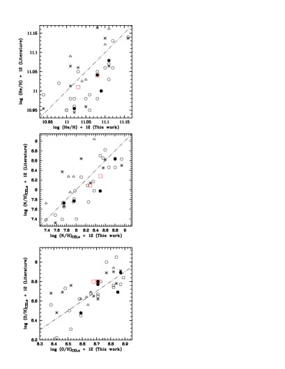
Figure 8: He, N and O abundances derived in the current work are compared to those in the literature for common objects. Filled circles: W88; Open circles: RPDM97; Open squares: CMKAS00; Open triangles: ECM04; Asterisks: EBW04.

Finally in a recent study, EBW04 determined abundances for a sample of 45 GBPNe, using a reduction procedure, set of atomic parameters and an ICF scheme that are almost identical to ours. Average abundances derived from their sample are in excellent agreement with ours, with differences less than 0.04 dex for He, O, S, about 0.1 dex for N and Ne and about 0.26 dex for Ar (c.f. Table 14).

5.2 Comparisons of abundances for common objects

Fig. 8 compares abundances of He, N and O determined in the current work with those published in the literature for common objects that were also observed and analyzed in the five other samples of GBPNe discussed above, but excluding the sample of EC01. CMKAS00 have only two objects in common with us, and the He and N abundances they obtained are about 0.03 and 0.21 dex lower than ours, whereas those of oxygen are 0.10 dex higher. The level of agreement is quite good, considering the measurement uncertainties involved. The numbers of common objects are 6, 20, 5 and 10 for the W88, RPDM97, ECM04 and EBW04 samples, respectively.

In term of systematic errors, abundances obtained by EBW04 are in best agreement with out results, although the scatter is also relatively large. The average abundance differences between the two samples are $0.00\pm 0.07$, $-0.09\pm 0.13$ and $0.10\pm 0.46$ dex for He, O and N, respectively, where the errors are standard deviations. For ECM04, the abundances they deduced for He and O for the five objects in common are in excellent agreement with our results, with average differences of $0.00\pm 0.10$ and $-0.02\pm 0.07$ dex, respectively. However, our nitrogen abundances are significantly lower than their results, by $-0.37\pm 0.21$ dex on average.

For objects in common with the W88 and with the RPDM97 samples, abundances of oxygen and nitrogen obtained in those studies are in good agreement with our results. For the W88 sample, the average differences are $0.03\pm 0.10$ and $0.26\pm 0.19$ dex for oxygen and nitrogen, respectively. For the RPDM97 samples, the corresponding values are $0.01\pm 0.22$ and $0.14\pm 0.23$ dex. However, both W88 and RPDM97 yield helium abundances that are systematically lower than our values, by $0.05\pm 0.03$ and $0.04\pm 0.04$ dex on average, respectively. The differences are found to mainly arise from measured line fluxes – for the same object, helium line fluxes measured by W88 and by RPDM97 are systematically lower than our values. For objects in common with RPDM97, if we recalculate helium abundances with our own method but using their line fluxes, the results are almost identical to their values. For the W88 sample, if we apply our analysis to her line data, the resultant helium abundances decrease by approximately 0.03 dex. This is caused by the fact W88 did not make any correction for the effects of collisional excitation of He i lines. Both W88 and RPDM97 applied non-linearity corrections to their line fluxes, measured, respectively, with the 3.9m Anglo-Australian Telescope using an Image Dissector Scanner as detector and with the ESO 3.6m or 1.52m telescopes also using an IDS. It is quite possible that both W88 and RPDM97 have over-corrected the effects of non-linearity, leading to underestimated fluxes for lines of low or intermediate strengths. If this was indeed the case, then intensities of the [O iii] $\lambda$4363 and [N ii] $\lambda$5754 auroral lines were also likely to have been underestimated, leading to underestimated $T_{\rm e}$, with apparent consequences to ionic abundances deduced for heavy elements.

6 CELs versus ORLs

As described in Section 1, plasma diagnostic analyses and elemental abundance determinations of PNe and H ii regions using CELs and ORLs/continua have ubiquitously showed dichotomy between results deduced from those two types of emission excited by different mechanisms. The discrepancies are generally characterized by $\Delta$$T_{\rm e}$, defined as $T_{\rm e}$([O iii])$-$$T_{\rm e}$(BJ), the difference between $T_{\rm e}$  deduced from the [O iii] collisionally excited lines and from the Balmer discontinuity of H i recombination spectrum, and by abundance discrepancy factor, adf, defined as the ratio of ionic abundances Xⁱ⁺/H⁺ derived from ORLs and from CELs. Deep optical spectroscopic surveys for dozens of GDPNe and a number of Galactic and extragalactic H ii regions have shown that values of $T_{\rm e}$(BJ) are systematically lower than those of $T_{\rm e}$([O iii]) deduced for the same objects and that adf’s are always larger than unity, falling typically in the range 1.6–3, but with a significant tail extending to higher values, reaching $\sim 70$ in the most extreme case. Except for the two GBPNe analyzed by Liu et al. (2001), ORL studies of PNe have so far concentrated on relatively bright GDPNe. The sample of GBPNe presented in the current work thus provides an interesting environment to probe the behaviours of the aforementioned fundamental discrepancies for a different stellar population. In particular, previous studies of GDPNe show that relative abundances of heavy elements, such as the C/O ratios deduced from ORLs are compatible to those derived from CELs. It is important to test whether the same result also holds for GBPNe.

6.1 Electron temperatures

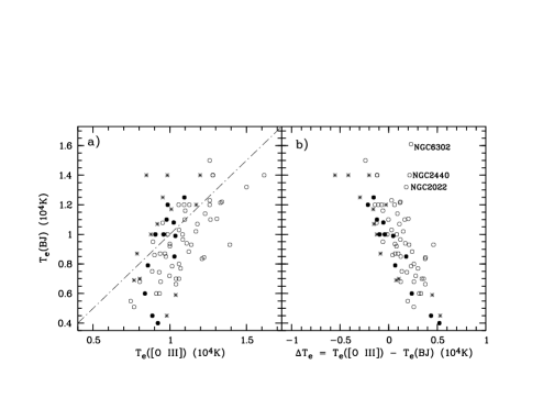
Figure 9: $T_{\rm e}$(BJ) plotted against a) $T_{\rm e}$([O iii]) and b) $\Delta T_{\rm e}\equiv$ $T_{\rm e}$([O iii])$-$$T_{\rm e}$(BJ) for GBPNe (filled circles and asterisks) and GDPNe (open circles). Filled circles and asterisks represent respectively GBPNe of sub-samples A and B, defined in Section 2.1. In a), the dotted-dashed diagonal line represents identical $T_{\rm e}$(BJ) and $T_{\rm e}$([O iii]).

In Figs. 9, 10 and 11, $T_{\rm e}$(BJ) is plotted against $T_{\rm e}$([O iii]), $\Delta$$T_{\rm e}$, $T_{\rm e}$(He i $\lambda 7281/\lambda 6678$) and against $T_{\rm e}$(O ii ORLs). Nebulae of sub-sample B, for which only low resolution spectra are available near the Balmer discontinuity region, do not behave obviously differently compared to objects of sub-sample A, although measurements for sub-sample B clearly suffer from larger uncertainties compared to the latter sub-sample. As a consequence, in analyses below we shall concentrate on patterns and relations revealed by sub-sample A.

A majority of our sample GBPNe (15 out of 25) have $T_{\rm e}$(BJ) higher than $T_{\rm e}$[O iii] (c.f. Fig. 9). For the sub-sample of high data quality, exactly half of the objects have $T_{\rm e}$(BJ) higher than $T_{\rm e}$([O iii]) while the other half have lower $T_{\rm e}$(BJ). The result appears to contradict to what previously found for GDPNe where for majority of them, $T_{\rm e}$(BJ) is systematically lower than $T_{\rm e}$([O iii]). Note that the magnitude of Balmer jump is inversely proportional to $T_{\rm e}$, thus as $T_{\rm e}$  increases, the Balmer jump becomes increasing difficult to measure. And because of the nonlinear dependence of $T_{\rm e}$(BJ) on the magnitude of Balmer jump, the resulting error of $T_{\rm e}$(BJ) for a given uncertainty of BJ is not symmetric – it biases towards higher values. It seems to us, at least parts, if not all, of the discrepant behaviour of GBPNe compared to GDPNe as seen in Fig. 9, are due to lower quality of the data available for GBPNe, which are generally fainter than nearby GDPNe.

While the left panel of Fig. 9 shows no obvious correlation between $T_{\rm e}$(BJ) and $T_{\rm e}$([O iii]), the right panel shows that there is a tight anti-correlation between $T_{\rm e}$(BJ) and $\Delta$$T_{\rm e}$  and different samples seem to yield similar results. Both panels however reflect the fact that while $T_{\rm e}$(BJ) varies over a wide range of values, $T_{\rm e}$([O iii]) falls within a much narrow range, as previously observed in GDPNe (c.f. Liu 2006a, b and references therein).

Fig. 10 compares $T_{\rm e}$(BJ) with $T_{\rm e}$(He i $\lambda 7281/\lambda 6678$), $T_{\rm e}$  derived from the ratio of He i singlet recombination lines $\lambda 7281$ and $\lambda 6678$. For all PNe plotted in the Figure, both disk and bulge ones, $T_{\rm e}$(He i $\lambda 7281/\lambda 6678$) is invariably lower than $T_{\rm e}$(BJ), in consistent with the expectations of the two-abundance model proposed by Liu et al. (2000), which predicts that $T_{\rm e}$(O ii ORLs) $\la$ $T_{\rm e}$(He i ORLs) $\la$ $T_{\rm e}$(H i BJ) $\la$ $T_{\rm e}$([O iii]) (Péquignot et al.2002; Péquignot et al. 2003; Liu 2003), exactly opposite to the expectations of the paradigm of temperature fluctuations which predict $T_{\rm e}$(He i $\lambda 7281/\lambda 6678$) $\ga$ $T_{\rm e}$(BJ) (Zhang et al.2005).

Fig. 11 plots $T_{\rm e}$(O ii ORLs) against $T_{\rm e}$(BJ), and again, in consistent with what previously found for GDPNe, values of $T_{\rm e}$(O ii ORLs) are considerably lower.

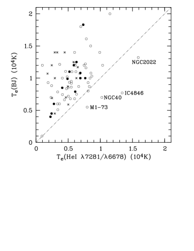
Figure 10: $T_{\rm e}$(BJ) plotted against $T_{\rm e}$(He i $\lambda 7281/\lambda 6678$), using the same symbols as in Fig. 9. The solid diagonal line represents $y=x$.

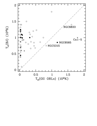
Figure 11: $T_{\rm e}$(BJ) plotted against $T_{\rm e}$(O ii ORLs) using the same symbols as in Fig. 9.

About half PNe in our GBPNe sample have an [O ii] $\lambda$4089/$\lambda$4649 line ratio higher than the low $T_{\rm e}$  limit of 288 K, the lowest $T_{\rm e}$  at which the effective recombination coefficients for O ii are available. (Tsamis et al.2004) detected a faint emission line at 4116 Å  in three bright PNe, NGC 3242, NGC 5882 and NGC 6818, and attributed it to Si iv 4s²S${}_{1/2}-$4p²P_1/2 $\lambda$4116.1. They corrected for the contribution of the other component of this multiplet, the 4s²S${}_{1/2}-$4p²P_3/2 $\lambda$4088.8 line, to the observed intensity of the O ii $\lambda$4089.3 line. After the corrections they obtained an $T_{\rm e}$(O ii  ORLs) of 2600, 8700 and 2900 K for NGC 3242, NGC 5882 and NGC 6818, respectively. For comparison, the H i Balmer jump temperatures they obtained for the three PNe are 10,200, 7800 and 12,100 K, respectively, and the corresponding values for $T_{\rm e}$([O iii]) are 11,700, 9400 and 13,300 K. The 4116 Å  feature has not been detected in NGC 6153 (Liu et al. 2000; adf = 9.7), in bulge PNe M 1-42 and M 2-36 (Liu et al. 2001; adf = 22.0 and 6.9, respectively) and in Hf 2-2 (Liu et al. 2006; adf = 71.2). For NGC 7009 (Liu et al. 1995; adf = 4.7), our unpublished deep spectra reveals a weak feature at 4116 Å. And if we apply similar corrections, then $T_{\rm e}$(O ii ORLs) yielded by the $\lambda 4089/\lambda 4649$ ratio increases from 420 K before the correction to 1310 K. For the sample of PNe observed and analyzed by (Liu et al.2004a, Liu et al.2004b), a line 4116.24 Å  rest wavelength was detected with a dereddened intensity of 0.029 (in units where H$\beta=100$) in the spectrum of NGC 6884 and was identified as [Ni v] $\lambda$4117.20. If we instead attribute it to Si iv $\lambda$4116, then $T_{\rm e}$(O ii  ORLs) yielded by the $\lambda 4089/\lambda 4649$ ratio will increase from the value of 3040 K before the correction to 22,100 K after the correction. Finally, amongst the large number of sample PNe studied by (Wesson et al.2005), the only PN that has a feature detected at 4116 Å  is Vy 2-2, with an observed intensity of $0.178$ in units of H$\beta=100$ after reddening corrections. However, the feature is unlikely to be Si iv $\lambda$4116 for two reasons: 1) If it is Si iv $\lambda$4116, then the other component of the multiplet at $\lambda$4089 should have an intensity of $2\times 0.178=0.356$, which is over a factor of three higher than the measured total intensity of the $\lambda$4089 feature (0.098); 2) The O⁺⁺/H⁺ ionic abundance ratio derived from the O ii $\lambda$4089 line, assuming no contamination from Si iv, is in good agreement with values deduced from other O ii ORLs. The case of Vy 2-2 suggests that the identification of the 4116 Å  features detected in some PNe as the Si iv $\lambda$4116 is not completely secure and further observations of better S/N’s and spectral resolutions are needed to clarify the situation.

6.2 Abundance discrepancy factors

The abundance discrepancy factor (adf) for a heavy element ionic species Xⁱ⁺ is defined as ratio of ionic abundance ratios Xⁱ⁺/H⁺ derived from ORLs and from CELs, adf(Xⁱ⁺) $\equiv$ (Xⁱ⁺/H⁺)_ORLs/(Xⁱ⁺/H⁺)_CELs. Previous studies of several samples of GDPNe show that adf varies over a wide range of values, from near unity (i.e. the ionic abundance ratios derived from the two types of emission lines agree) to over a factor of ten, peaking around a factor of two but with a tail extending to much higher values, reaching a factor of $\sim 70$ in the most extreme case (c.f. Liu 2006a, b).

In Fig. 12 we plot and compare the accumulative distributions of adf for disk PNe from the TLW (c.f. Section 7) sample and for bulge PNe from the current sample. The two distributions show some differences for adf(O²⁺) between 0.5 and 0.8 dex. A Kolmogorov-Smirnov Two-sample test, with the Null Hypothesis that the two samples have the same distributions of adfs, yields a Kolmogorov-Smirnov statistic $D$ of 0.1808 with a probability of the two distributions having a difference exceeding $|D|$ under the Null Hypothesis, $P(>|D|)=0.59$, which is equal to 1 minus the confidence level. In other words, the risk is high, nearly 60 per cent, to reject the Null Hypothesis. The analysis thus shows that to a fairly good confidence level, both GDPNe and GBPNe seem to yield similar distributions of adf(O²⁺).

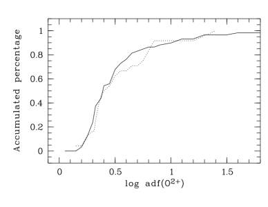
Figure 12: Comparison of the accumulative distributions of $\log\,{\rm adf}({\rm O}^{2+})$ of GDPNe (solid line) and of GBPNe (dotted line).

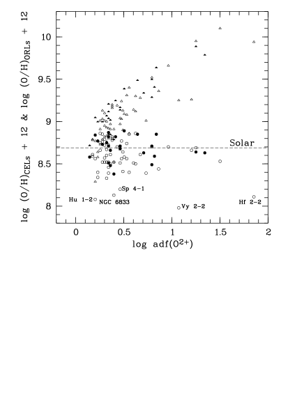
Figure 13: Elemental abundances of oxygen derived from ORLs (triangles) and from CELs (circles) plotted against adf(O²⁺) for GBPNe (filled symbols) and GDPNe (open symbols). The solar photospheric oxygen abundance (Lodders 2003) is marked.

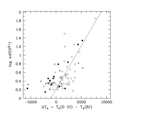
Figure 14: adf(O²⁺) plotted against $\Delta$$T_{\rm e}$. For the meaning of different symbols, c.f. Fig. 9. The solid line shows the linear fit obtained by Liu et al. (2001).

In Fig. 13, we plot total elemental abundances of oxygen derived from CELs and from ORLs against adf(O²⁺). The Figure shows that except for a few PNe with O/H less than 8.2, oxygen abundances derived from CELs fall into a relatively narrow range, consistent with the general consensus that oxygen is neither created nor destroyed by any significant amount in LIMS. By contrast, oxygen abundances yielded by ORLs, apart from being always higher than the corresponding values derived from CELs for the same object, cover a wide range of values, reaching about a factor of 25 higher than the solar value in the most extreme case. Such high abundances are extremely difficult to explain in terms of the current theory of evolution of low- and intermediate-mass (single) stars, and argue strongly against the paradigm of temperature fluctuations as the underlying physical cause of the large adf values, as the scenario implicitly assumes that the higher abundance values yielded by ORLs, being insensitive to the presence of temperature fluctuations, are the correct values (c.f. Liu 2006b). Together with Fig. 9, Fig. 13 also implies that whatever effects are causing the large values of adf observed in PNe, it seems they manifest themselves mainly by affecting emission of ORLs/continua, leading to large variations in $T_{\rm e}$  and ionic abundances that are inferred from emission of ORLs/continua.

Fig. 14 plots $\log$ adf(O²⁺) against $\Delta$$T_{\rm e}$. Also overplotted is the linear fit obtained for a much smaller sample of PNe by Liu et al. (2001) who first noticed that the two quantities are positively correlated. The result suggests that both phenomena, i.e. that $T_{\rm e}$  derived from the [O iii] forbidden lines are systematically higher that those derived from the Balmer discontinuity of the H i recombination spectrum, and that ionic abundance ratios of heavy elements derived from ORLs are systematically higher than deduced from CELs, are related and probably caused by the same underlying physical mechanism. Furthermore, from the discussion above, we may conclude that the mechanism, whatever it is, affects mainly the emission of ORL/continua, rather than that of CELs. The results fit nicely with the expectations of the two-abundance model proposed by Liu et al. (2000), but contradict those of the paradigm of temperature fluctuations which affect mainly the production of emission of CELs.

The mean surface brightness reflects the evolutionary stage of a PN. As the PN evolves and expands, its density drops and thus the surface brightness. Garnett & Dinerstein (2001) found that adf(O²⁺) tends to be larger for bigger, lower surface brightness PNe. A similar trend was found by (Liu et al.2004b). In Fig. 15, we plot adf(O²⁺) against the nebular 6 cm radio surface brightness, defined as $F(5\,{\rm GHz})/\theta^{2}$, where $F(5\,{\rm GHz})$ is nebular 6 cm radio flux density in mJy and $\theta$ is angular diameter in arcsec (c.f. Table 1). Using radio flux density instead of H$\beta$ flux has the advantage that the former is not affected by interstellar extinction. Although with large scatter, the diagram shows some evidence that adf increases with decreasing surface brightness, consistent with previous results.

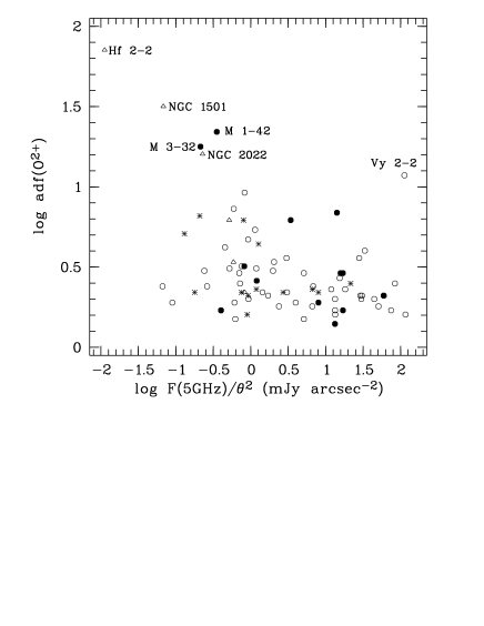
Figure 15: adf(O²⁺) plotted against radio band surface brightness at 6 cm. For the meaning of different symbols, c.f. Fig. 9. For a few PNe that have no measurements of 5 GHz radio flux density, we have adopted 1.4 GHz fluxes and converted the values to 5 GHz fluxes assuming optically thin emission. Those objects are marked with triangles.

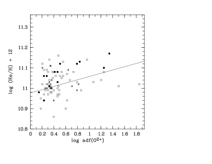
Figure 16: Helium abundance plotted against adf(O²⁺). For the meaning of different symbols, c.f. Fig. 9. The solid line represents the linear fit obtained by (Liu et al.2004b).

(Zhang et al.2004) found a positive correlation between $\Delta T_{\rm e}$ and helium abundance, in accordance with the expectations of the two-abundance model. Our current data for GBPNe exhibit a similar trend, albeit with larger scatter due to the larger uncertainties associated with the current determinations of $T_{\rm e}$(BJ) (c.f. §2.1). Fig. 16 plots He abundance against adf(O²⁺). The solid line in the Figure shows the linear regression obtained by (Liu et al.2004b) for disk PNe. Again, while the scatter is large, there is a discernible positive correlation between the two quantities.

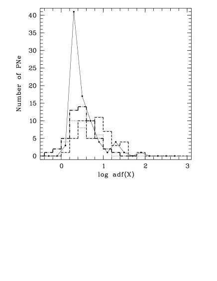
Figure 17: Comparison of the distributions of $\log$ adf for O²⁺/H⁺ (solid curve), C²⁺/H⁺ (dashed-dotted histogram), N²⁺/H⁺ (dotted histogram) and Ne²⁺/H⁺ (dashed histogram) ionic abundance ratios.

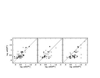
Figure 18: $\log$ adf of O²⁺ plotted against those of C²⁺, N²⁺ and Ne²⁺ for GBPNe (filled circles) and GDPNe (open circles). The solid lines represent $y=x$.

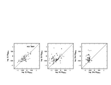
Figure 19: Comparison of heavy element abundance ratios C/O, N/O and Ne/O derived from ORLs and from CELs, for GBPNe (filled circles) and GDPNe (open circles). The solid lines represent $y=x$.

It has been shown that apart from oxygen, the large discrepancies between ionic abundances relative to hydrogen derived from ORLs and from CELs exist for the other three abundant second-row elements, carbon, nitrogen and neon (Liu et al. 1995; Luo et al.2001). In addition, for a given PN, values of the adf deduced for the four most abundant second-row heavy elements are comparable (Liu et al. 2000). In other words, both CEL and ORL analyses yield similar relative abundance ratios of heavy elements, such as C/O, N/O and Ne/O. Fig. 17 shows the distributions of $\log$ adf(X), where X = C²⁺/H⁺, N²⁺/H⁺, O²⁺/H⁺ and Ne²⁺/H⁺, for all Galactic PNe for which a measurement of the quantity is available. The distribution of adf(O²⁺) peaks strongly near 0.3 dex, with a FWHM of 0.26 dex and an extended tail towards higher values. For C²⁺/H⁺ and N²⁺/H⁺, the distributions peak around 0.5 dex with a FWHM of about 0.7 and 1.0, respectively. For Ne²⁺/H⁺, it peaks around 0.8 dex with a FWHM of 1.2 dex. In Fig. 18, we plot the adf deduced for O²⁺/H⁺ against those of C²⁺/H⁺, N²⁺/H⁺ and Ne²⁺/H⁺. The Figure shows that adf(C²⁺) follows closely adf(O²⁺), whereas adf(N²⁺) and adf(Ne²⁺) are systematically higher than adf(O²⁺). Heavy element abundance ratios, C/O, N/O and Ne/O, derived from CELs and from ORLs, are compared in Fig. 19. In line with the patterns revealed in Fig. 18, both CELs and ORLs yield compatible C/O abundance ratio, whereas for N/O and Ne/O, the ratios deduced from ORLs are systematically higher, a direct consequence of higher values of adf found for N²⁺/H⁺ and Ne²⁺/H⁺. The average C/O ratios found from ORLs are $-0.11\pm 0.05$ for GDPNe (39 objects) and $-0.38\pm 0.06$ for GBPNe (13 objects). The corresponding results from CELs are $-0.19\pm 0.05$ and $-0.35\pm 0.10$ for GDPNe and GBPNe, respectively. In the scenario of two-abundance scenario proposed by Liu et al. (2000), ORLs and CELs trace respectively the cold, H-deficient inclusions and the hot, diffuse medium of normal composition. The fact that both ORLs and CELs yield compatible C/O ratios suggests that the postulated H-deficient inclusions have the same C/O ratio as the diffuse medium and therefore unlikely to be nucleo-processed material as proposed by Iben et al. (1983) for H-deficient knots observed in Abell 30 and Abell 78. Deep spectroscopy and ORL abundance analysis of H-deficient knots in Abell 30 (Wesson et al.2003) also show that the knots are O-rich rather than C-rich, in contradiction to predictions of the born-again scenario proposed by Iben et al. (1983).

Fig. 19 also shows the C/O ratio varies over a factor of ten, from $-0.5$ to $+0.5$ dex, and that C/O ratios of GBPNe are systematically lower than those of GDPNe. This important result will be discussed further in the next Section.

For the four abundant second-row elements, adf(O²⁺) is probably the best determined. First of all, high quality calculations of effective recombination coefficients for the whole range of O ii ORLs are available (Liu et al. 1995). Those calculations have been extended down to a $T_{\rm e}$  as low as 1000 K and even to 288 K for some selective transitions (Bastin 2006). Secondly, most prominent O ii ORLs fall within the narrow 4000–5000 Å  optical wavelength range where one also finds the three [O iii] CELs, the $\lambda\lambda$4959,5007 nebular lines and the $\lambda$4363 auroral line, upon which CEL analysis relies. All those lines can thus be measured simultaneously using a single instrument and sampling the same area of a given nebula. This avoids or minimizes errors caused by effects such as uncertainties in flux calibration and reddening corrections. For carbon, good atomic data also exist for C ii ORLs (Davey et al. 2000) and the lines are generally well measured, in particular the relatively strong 3d–4f $\lambda$4267 transition, yielding fairly accurate C²⁺/H⁺ ratios. On the other hand, for CEL analysis, the derivation of carbon ionic abundance ratios has to rely on UV CELs, most importantly, the C iii] $\lambda\lambda$1907,1909 for C²⁺/H⁺ and C iv $\lambda\lambda$1548,1550 for C³⁺/H⁺. Thus except for a number of extended PNe for which the optical spectra have been obtained by scanning the whole nebula (e.g. Liu et al. 2000; Tsamis et al.2004), and for those nebulae of small angular sizes ($\la$ a few arcsec, such as most GBPNe) and nearly symmetric, the adf(C²⁺) deduced may suffer from errors. These uncertainties result from the fact that the UV and optical observations may not be sampling the same portions of the nebula as well as from potential uncertainties in flux normalization and reddening corrections.

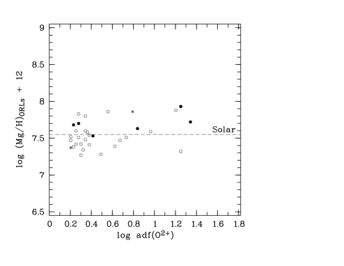
Figure 20: Magnesium abundance, Mg/H $\approx$ Mg²⁺/H⁺, with the later derived from the Mg ii $\lambda$4481 ORL, plotted against adf(O²⁺). The solar photospheric magnesium abundance (Lodders 2003) is marked. For an explanation of different symbols, c.f. Fig. 9.

Good atomic data now exist for $l\leq 2$ transitions of N ii (Kisielius & Storey 2002) and Ne ii (Kisielius et al.1998) ORLs, but not those arising from levels of higher orbital angular momenta, such as 3d–4f lines. N ii and Ne ii ORLs are generally much more difficult to observe than O ii ORLs due to lower abundances of nitrogen and neon compared to oxygen. Most of the strongest Ne ii 3–3 transitions fall at shorter wavelengths below 4000 Å. Whereas Ne²⁺/H⁺ can be deduced from strong optical [Ne iii] $\lambda\lambda$3868,3967 nebular lines, N²⁺/H⁺ can only be obtained from either the relatively weak N iii] $\lambda$1751 intercombination line or from the [N iii] 57$\mu$m far-infrared lines. All those factors make the current estimates of adf(N²⁺) and adf(Ne²⁺) subject to large uncertainties. We believe that a major fraction, if not all, of the larger values of adf found for N²⁺/H⁺ and Ne²⁺/H⁺ compared to adf(O²⁺) (Fig. 18) and consequently, higher N/O and Ne/O ratios yielded by ORLs compared to those obtained from CELs (Fig. 19), are caused by those uncertainties and are therefore artificial. Better observations and atomic data for N ii and Ne ii ORLs are clearly needed. More accurate determinations of N/O and Ne/O ratios using ORLs are of great interest to unveil the nature and origins of the postulated H-deficient inclusions embedded in the diffuse nebula that are responsible for large values of adf observed in PNe.

Magnesium is the only third-row element for which an ORL from one of its dominant ionic species has been detected, i.e. the Mg ii 3d–4f $\lambda$4481 line yielding Mg²⁺/H⁺. To a good approximation, Mg/H $\sim$ Mg²⁺/H⁺ (Barlow et al. 2003). Mg/H abundances thus deduced are now available for a total of 32 PNe, including 24 GDPNe and 8 GBPNe (excluding the peculiar M 2-24; Zhang & Liu2003). The results are plotted in Fig. 20 against adf(O²⁺). Mg/H abundance is particularly difficult to obtain from CELs, as it has to rely on weak lines in the UV or in the infrared. Thus adf(Mg²⁺) cannot be deduced. However, as previously noticed by Barlow et al. (2003), in stark contrast to C, N, O and Ne, for a wide range of adf(O²⁺), Mg/H deduced from the Mg ii $\lambda$4481 ORL fall in a narrow range compatible with the solar photospheric value. The 24 GDPNe plotted in Fig. 20 yield an average Mg/H ratio of 7.56 dex with a standard deviation of 0.22 dex, almost identical to the solar value of 7.55 (Lodders 2003). The 8 GBPNe yield a slightly higher average value, of 7.71 dex. We will discuss magnesium abundance in the context of the chemical evolution of the Galaxy in the next Section.

6.3 Summary

In summary, the current detailed plasma diagnostics and abundance analyses contrasting results obtained from CELs and those deduced from ORLs and continua for a large sample of GBPNe have yielded the same phenomena and strengthen the conclusions previously found for GDPNe:

1) Nebular electron temperatures deduced from recombination lines or continua are systematically lower than those deduced from the classic [O iii] nebular to auroral forbidden line ratio. In addition, there is strong evidence that $T_{\rm e}$  derived from He i ORL ratios, $T_{\rm e}$(He i), are systematically lower than $T_{\rm e}$(BJ), $T_{\rm e}$  deduced from the H i recombination continuum Balmer discontinuity, and that $T_{\rm e}$  given by recombination line ratios of heavy element ions, such as from O ii ORL ratios, are even lower, yielding values that are just a few hundred K in some cases.

2) Heavy element abundances relative to hydrogen derived from ORLs are always higher than values derived from CELs. This is true for all abundant second-row elements, C, N, O and Ne. For a given nebula, values of the adf found for those individual elements are comparable, leading to similar values of abundance ratios, C/O, N/O and Ne/O deduced from ORLs and from CELs. By contrast, no enhancement of ORL abundances relative to CEL values is apparent for magnesium, the only third-row element that has been studied using ORLs. There is also evidence that objects exhibiting particularly large values of adf also have higher helium abundances.

3) The observed discrepancies between $T_{\rm e}$  and heavy element abundances derived from ORLs and from CELs are correlated. Objects showing large values of adf tend to have large $T_{\rm e}$  discrepancies, suggesting that the two phenomena are related, and are likely caused by the same underlying physical process.

4) The large discrepancies between $T_{\rm e}$  derived from CELs and from ORLs appear to be mainly caused by abnormally low values yielded by recombination lines or continua. For the large number of nebulae analyzed, $T_{\rm e}$  derived from CELs fall in a narrow range around 10,000 K, consistent with what is predicted by photoionization models for nebulae of “normal” chemical composition, i.e. that of Sun, a typical G-dwarf in the Galaxy. Similarly, the large discrepancies between heavy element abundances deduced from ORLs and from CELs are largely caused by the abnormally high values obtained from ORLs. Excluding a few nebulae that are known to belong to the halo population and thus have lower heavy element abundances, abundances of most PNe deduced from CELs fall in a narrow range of slightly sub-solar. By contrast, ORLs yield much higher heavy element abundances, reaching more than a factor of ten higher than the solar values in some extreme cases. It appears that whatever is causing the large differences between results obtained from ORLs and from CELs, the main effect of the process is to enhance emissivities of recombination lines and continua, but hardly affect those of CELs. The results also suggest that heavy element abundances deduced from ORLs are unlikely to be real, or representative of the bulk composition of the whole nebula. This is in stark contradiction to the prediction of the paradigm of temperature fluctuations, which implicitly assumes that the higher abundances yielded by ORLs are the correct ones.

5) All the above results point to the existence of a cool component of metal-rich plasma embedded in the diffuse nebula, as first proposed by Liu et al. (2000). The cool inclusions are responsible for most of the observed fluxes of ORLs emitted by heavy element ions, yet contribute little to the fluxes of CELs. As the nebula expands and ages, the diffuse emission fades and emission from the embedded cool inclusions becomes more apparent.

7 Discussion

In this Section, we compare elemental abundances deduced for the current sample of GBPNe with those derived previously for GDPNe. We investigate the abundance patterns and discuss the results in the context of the nucleosynthesis and dredge-up processes in LIMS and their roles in the chemical evolution of the Galaxy. Of the GBPNe observed in the current work (Table 1), we have excluded in our analysis the peculiar nebulae M 2-23 and M 2-39 (c.f. § 3.3), but included M 2-36 and M 1-42 previously studied by Liu et al. (2001). The sample, WL07, consists of 25 bulge PNe in total.

As described in § 1, deep spectroscopy, contrasting plasma diagnostic and abundance analysis results obtained from the traditional method based on strong CELs with those based on much fainter ORLs, has been carried out for three samples of GDPNe (Tsamis et al.2003; Tsamis et al.2004, 12 PNe, TBLS04 hereafter; Liu et al.2004a, Liu et al.2004b, 12 PNe, LLBL04 hereafter; Wesson et al.2005, 23 PNe, WLB05 hereafter). In addition, case studies for a number of individual PNe have been published, some of them showing particularly prominent and rich ORL spectra from heavy element ions. They include NGC 7009 (Liu et al. 1995; Luo et al.2001), NGC 6153 (Liu et al. 2000), NGC 6543 (Wesson & Liu2004), Me 1-1 (Shen et al. 2004), NGC 1501 (Ercolano et al. 2004), NGC 7027 (Zhang et al.2005) and Hf 2-2 (Liu et al. 2006). In the current work, six PNe observed belong to the disk population (c.f. Table 1). In all the studies, the nebulae were observed using low- to intermediate-resolution long-slit CCD spectrophotometry and then analyzed in a similar manner (plasma diagnostics, atomic data and ICF scheme). All those disk PNe, including six from the current work, are grouped to form a homogeneous sample of GDPNe to compare with the current sample of GBPNe. A few nebulae observed and analyzed using similar techniques were excluded, either because of their peculiarities, e.g. Abell 30 (Wesson et al.2003), Mz 3 (Zhang & Liu2002), M 2-24 (Zhang & Liu2003), or because the objects actually belong to a different population, e.g. NGC 4361 (Liu 1998) and DdDm 1 (WLB05); both are believed to be halo PNe. We note that fluxes for a number of lines published by WLB05 for PN M 3-27 seem to be incorrect. We have therefore remeasured the lines and repeated the analysis. In total, our final sample of GDPNe consists of 58 PNe and will be referred to hereafter as TLW (‘T’ for TBLS04, ‘L’ for LLBL04 and ‘W’ for WLB05 – the three samples constituting the majority of the TLW sample).

We note that most of the objects observed by TBLS04 are within the solar circle, whereas the northern PNe in the WLB05 sample are mostly outside the solar circle, and the LLBL04 sample is a mixture. The mean O/H abundances deduced from the three samples are 8.70, 8.58 and 8.60, respectively. The corresponding values after excluding Type-I PNe (and the very low excitation PN in the WLB05 sample) are 8.74, 8.57 and 8.59, respectively. The small variations of mean oxygen abundances between the samples thus reflect an abundance gradient across the Galactic disk. We also note that the average metal abundances yielded by the KB94 sample of disk PNe are systematically higher than those from the TLW sample, varying from about 0.1 dex for oxygen, neon and sulfur to about 0.2 dex for carbon, nitrogen and argon. Part of the differences may be caused by abundance gradients across the disk. Most PNe in the KB94 sample are southern hemisphere nebulae and therefore within the solar circle. For the 38 and 16 PNe within and outside the solar circle in the KB94 sample, the mean oxygen abundances are 8.71 and 8.60, respectively.

7.1 Comparison between bulge and disk samples

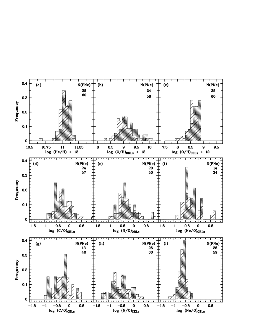
Figure 21: Distributions, normalized to unit area, of elemental abundances relative to hydrogen, and of heavy element abundance ratios for GDPNe (lightly shaded histograms) and GBPNe (heavily shaded histograms). The ordinate gives the fractional number of nebulae in each bin. The bin size is 0.05 for panel (a) and 0.10 for all the other panels. In each panel, numbers of bulge and disk PNe for which measurements are available are marked from top to bottom.

Table 14 shows that compared to the disk PN sample TLW, the average elemental abundances of the bulge PN sample WL07, are consistently higher, except for C/H derived from ORLs and Cl/H deduced from CELs. If we define $\Delta M({\rm X})$ as the difference between the average abundances of element X relative to H derived from disk bulge sample WL07 and from the disk sample TLW, $\Delta M({\rm X})\equiv M({\rm X},{\rm GBPNe})-M({\rm X},{\rm GDPNe})$, then $\Delta M({\rm X})$ ranges from 0.04 dex for He/H from ORLs, 0.10 dex for O/H from both CELs and ORLs, $\sim 0.15$ dex for Ne/H and Ar/H from CELs, 0.15 dex for Mg/H from ORLs, 0.17–0.20 for N/H from CELs and from ORLs, and 0.21 dex for S/H from CELs.

Fig. 21 compares distributions, normalized to unit area, of elemental abundances relative to hydrogen and of heavy element abundance ratios for the WL07 bulge sample (heavily shaded histograms) and the TLW disk sample (lightly shaded histograms). Panels (a) – (c) of Fig. 21 show that abundances of He and O of bulge PNe peak at higher values compared to disk PNe. Panels (d) and (g) show that, as already pointed out in §6.2 (c.f. Fig. 19), bulge PNe have lower C/O ratios than disk PNe, by approximately 0.2 dex. On the other hand, bulge and disk PNe seem to have similar distributions of N/O and Ne/O abundance ratios (as discussed in §6.2, nitrogen and neon abundances deduced from ORLs and consequently N/O and Ne/O abundance ratios based on ORLs are less reliable compared to those of carbon and oxygen).

It is generally accepted that abundances of oxygen, neon, sulfur and argon are hardly affected by nucleosynthesis and dredge-up processes that occur in progenitor stars of PNe, thus their abundances should reflect values of the ISM at the time those LIMS were formed. For these four elements, their average abundances deduced from CELs for the bulge sample WL07 are consistently higher by $\sim 0.1$–0.2 dex than for the disk sample TLW. Corroborating evidence is provided by the average O/H abundances derived from ORLs for which good atomic data exist and line measurements are reasonably reliable. The results show that the bulge is slightly overabundant with respect to the disk, by approximately 0.1 dex. Although the inferred abundance differences between the bulge and disk samples are small, the consistency of results for all $\alpha$ elements measured as well as from different tracers (CELs versus ORLs) strongly suggests that differences are probably meaningful.

Supporting evidence that the Galactic bulge is more metal-rich than the disk has also been found from other independent abundance studies of bulge PNe. Spectrophotometric abundance analyses of 30 GBPNe by CMKAS00 show that while the average abundances of O, S and Ar of GBPNe are comparable to those of GDPNe, there is some evidence that higher elemental abundances are slightly more frequently found amongst the bulge PNe. More recent work on 44 GBPNe by (Górny et al.2004) also came to the same conclusion. They compared the average oxygen abundance of their sample b (bulge PNe) with sample d (disk PNe within the solar circle compiled from the literature) and found that the former is about 0.13 dex (or 0.2 dex) more metal abundant than the latter. Their findings are roughly in agreement with our results. Note that there are only a handful of common objects between the three samples of bulge PNe and independent analyses all indicate that GBPNe are slightly more metal-rich than GDPNe.

The lower C/O ratios observed in GBPNe compared to GDPNe may suggest that GBPNe evolve from more massive progenitor stars. As a consequence, a larger fraction of carbon has been converted to nitrogen, although it is difficult to rule out selection effects as PNe of less massive cores are also less bright and therefore harder to observe, particularly those in the distant, heavily extincted region of the Galactic bulge. Alternatively, it may indicate that the 3rd dredge-up process is less efficient for metal-rich GBPNe than for GDPNe. In § 7.2, we will discuss in detail the lower C/O ratios measured for GBPNe and compare the results with some of the recent theoretical predictions.

The distribution of He/H, O/H and Ne/O abundance ratios plotted in Fig. 21 can be well fitted using a single Gaussian profile, while those of C/O and N/O appear to be more irregular and double-peaked. While observational errors may play a role, the results may indicate that there are two populations in each of the two samples. A scrutiny of N/H abundances obtained by EBW04 for a sample of GBPNe (see the solid histograms in their Fig. 4) also reveals a double-peak distribution, peaking at 8.1 and 8.7 dex, respectively, similar to what we find for the current sample of GBPNe. Similarly, N/H abundances of the ECM04 sample also exhibit two local maxima, at 7.7 and 8.4 dex, respectively. It is interesting to note for each of the three samples of GBPNe, the two local maxima observed in the N/H abundance distribution are consistent with the average N/H abundance ratios for non-Type I and Type-I PNe in the corresponding sample, respectively. The fraction of Type-I PNe in the WL07 bulge PN sample is 19 per cent, very similar to the fraction of 21 per cent for the TLW disk sample. It seems unlikely that the slightly higher metallicity observed for GBPNe compared to GDPNe is caused by a mixture of different populations in the two samples.

In a recent theoretical study, (Nakasato & Nomoto2003) have modelled the Galaxy formation using three-dimensional, hydrodynamic N-body simulations, paying particular attention to the formation of the bulge component. Their simulations show that the bulge consists of two chemically different components – one resulted from a fast merging of subgalactic clumps in the proto-Galaxy while the other formed gradually in the inner disk. Their results predict a double-peak [Fe/H] abundance distribution – the iron content in the non-merger component is higher than the merger component as a result of pollution by Type-Ia supernovae. It is unclear however how the double-peak [Fe/H] distribution predicted for the bulge is related to the double-peak distribution of N/H abundances observed in GBPNe.

To summarize, a comparison of elemental abundances of disk and bulge PNe shows that GBPNe appear to be more metal-rich than GDPNe, by approximately 0.1 – 0.2 dex. In addition, the mean C/O ratio of GBPNe are lower than that of GDPNe, by 0.16 and 0.27 dex as deduced from CELs and ORLs, respectively.

7.2 Carbon and nitrogen

At the end of the main-sequence evolution when the central hydrogen is exhausted, the star evolves to the red giant branch (RGB). A convection zone develops and dredge-ups partially CN-cycle processed material to the surface. This first dredge-up process enhances the surface nitrogen abundance and reduces the surface abundance of carbon as well as the ¹²C/¹³C isotope ratio. Following the exhaustion of central helium and the formation of an electron degenerate CO core, the second dredge-up starts in early Asymptotic Giant Branch (AGB) stars but only in those more massive ones with initial masses in the (uncertain) range from 2.3 to 8 $M_{\sun}$. The process increases the surface abundances of both helium and nitrogen and reduces slightly those of carbon and oxygen. The third dredge-up takes place in AGB stars during the thermal pulses (helium shell flashes). Helium-burning products, mostly ¹²C and s-process elements, are brought to the surface. On the way to the surface, the material is subject to limited CN-cycle burning, allowing for some conversion from C to N and decreasing the ¹²C/¹³C ratio. In all three episodes of the dredge-up process, the surface abundances of He and N are increased, while that of ¹²C abundance and the ¹²C/¹³C isotope ratio first decrease in the first (and second, when it occurs) dredge-up episode and then increase in the third. The amount of abundance changes depends mainly on the initial mass but also on metallicity of the progenitor star. The abundances of C and N relative to other light elements thus provide tools to probe the nucleosynthesis and mixing processes as well as properties of PN progenitor stars, such as their initial masses and metallicities.

Since the pioneering work by (Renzini & Voli1981), the roles of LIMS in enhancing the chemical composition of the ISM have been studied extensively, both observationally and theoretically. In recent work, Marigo (2001, Ma01 hereafter) presented quantitative predictions of the surface abundance patterns of He, C, N and O for different values of initial stellar mass and metallicity and mixing-length parameter $\alpha$.

In Figs. 22, 23 and 24, we plot N/O ratios measured for the WL07 sample of GBPNe and for the TLW sample of GDPNe, deduced from CELs and from ORLs against He/H derived from ORL analysis and against N/H and O/H obtained from CEL analysis. The data are compared with theoretical tracks calculated by Ma01 as a function of initial mass for initial metallicities $Z=0.04$, 0.008 and 0.019, assuming $\alpha=1.68$.

Fig. 22 shows that the observed distribution of N/O versus He/H does not fit well with what is expected, with many data points falling to the upper left of the theoretical tracks. Either the theoretical calculation underestimates the N/O ratio or overestimates the He/H enhancement, assuming that most PNe are descendants of LIMS, an assumption which is most likely true. The effect is most obvious for GDPNe (open symbols). Similarly, Fig. 23 shows that while most GBPNe (filled symbols) fall within the band delineated by the tracks of various initial metallicities, more than half the open symbols fall above and to the left of the track of even the lowest metallicity $Z=0.004$. The theoretical loci of N/O versus O/H become almost orthogonal to the abscissa (Fig. 24) for initial masses higher than $\sim 2~{}M_{\odot}$. Again in this diagram, we find that bulge PNe are mostly found between the two loci for initial $Z=0.008$ and 0.016, while a significant fraction of disk PNe fall to the left of the loci for $Z=0.004$. Figs. 22, 23 and 24 thus all seem to indicate that bulge PNe originated from environments of higher metallicities ($Z\sim 0.013$ from a rough estimate) than disk PNe. In addition, Fig. 23 shows that to reach a given value of the N/O ratio, a much higher initial mass is required for a star of higher initial metallicity than for one of lower initial metallicity. Fig. 23 shows that almost all disk PNe appear to evolve from stars of initial mass lower than $\sim 4~{}M_{\odot}$ (assuming they have an initial metallicity close to or lower than 0.008), while a significant fraction of bulge PNe have initial masses higher than this. We thus conclude that PNe of massive progenitors are more frequently found in the bulge than in the disk, at least for the limited sample of bulge PNe analyzed in the current work.

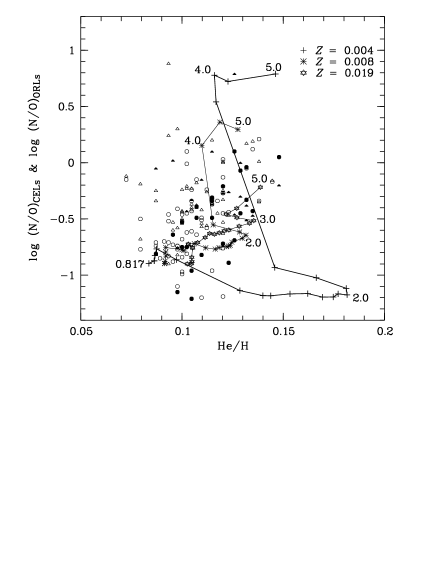
Figure 22: N/O abundance ratios derived from CELs (circles) and from ORLs (triangles) for the WL07 sample of GBPNe (filled symbols) and the TLW sample of GDPNe (open symbols), plotted against helium abundance He/H. Overplotted are loci of initial mass predicted by Ma01 for initial metallicities $Z=0.004$, 0.008, 0.019 and mixing length parameter $\alpha=1.68$. The tick marks on the tracks indicate initial stellar mass, ranging from $\sim 0.8$ to 5 $M_{\odot}$. Only a few values are labelled.

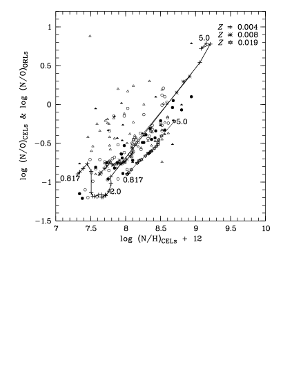
Figure 23: N/O abundance ratios plotted against N/H abundance. For an explanation of the different symbols and lines, c.f. caption to Fig. 22.

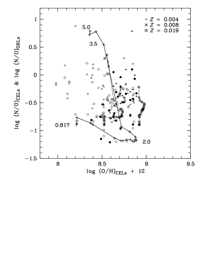
Figure 24: N/O abundance ratios plotted against O/H abundance derived from CELs. For an explanation of the different symbols and lines, c.f. caption to Fig. 22.

Loci of the C/O ratio versus He/H and O/H abundances calculated by Ma01 are plotted in Figs. 25 and 26, respectively, and compared to observations. For low-mass progenitor stars, in the absence of Hot-Bottom-Burning (HBB) which destroys carbon, the final surface abundance of carbon as well as the C/O ratio increase with increasing initial mass, as a result of the increasing number of dredge-up episodes experienced during the Thermal-Pulse-AGB phase. The quantities reach maximum values around 2–3$M_{\odot}$. Beyond that, they start to decline as initial mass increases as a consequence of less dredge-up events. For even higher initial masses, HBB kicks in and eventually prevails.

As noted earlier (§6.2, Fig. 19), GBPNe appear to have lower C/O ratios than GDPNe. Fig. 25 shows that the majority of GBPNe have C/O ratios lower than the predicted values of Ma01 for initial values ranging from $\sim 0.8$–5 $M_{\odot}$. Even for GDPNe, over half of them have C/O ratios lower than the lowest predicted values. Similar trends are also found in Fig. 26. Thus, it sees that the theoretical calculations of Ma01 have overestimated the yield of carbon, by as much as about 0.4 dex. The predicted C/O ratios can be lower for initial masses higher than 5 $M_{\odot}$. However, it seems highly unlikely that over half the PNe in our sample descend from such massive stars.

Fig. 26 can be used to obtain better estimates of the average initial metallicity for our disk and bulge PN samples than possible with Fig. 24, because the C/O ratio is more sensitive to the initial metallicity than N/O is. Fig. 26 shows that essentially all PNe in our sample of GBPNe fall between the two loci of $Z=0.008$ and 0.019, while most PNe in the current sample of GDPNe fall close to the locus of $Z=0.008$.

In summary, both from the actually observed distributions of oxygen abundances (Fig. 21) for bulge and disk PNe as well as from the measured N/O and C/O abundance ratios (Figs.  23, 24 and 26), there is strong evidence indicating that GBPNe were formed in environments of higher metallicities ($Z\sim 0.013$) compared to disk PNe. The latter seem to have initial metallicities $\la 0.008$. We also find that the current sample of GBPNe may originate from more massive stars than the disk PNe. Finally, we point out that Ma01 may have overestimated carbon yield by over a factor of two.

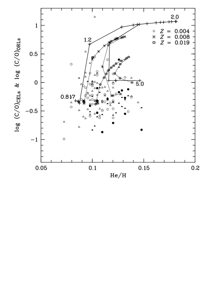
Figure 25: C/O abundance ratios derived from CELs and from ORLs plotted against helium abundances for bulge and disk PNe. Overplotted are loci calculated by Ma01. See also the caption to Fig. 22 for more description.

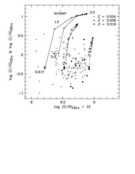
Figure 26: C/O ratios derived from CELs and from ORLs plotted against oxygen abundances derived from CELs for GBPNe and GDPNe. See also the caption to Fig. 22 for more description.

7.3 Oxygen, neon and argon

There is a tight linear relation between neon and oxygen abundances as illustrated in Fig. 27. The only exception is Sp 4-1 (WLB05). For this peculiar object, with the exception of oxygen, its abundances of all other heavy elements are lower than the average of disk PNe by 0.5 to 0.8 dex. Similar correlations between the neon and oxygen abundances have previously been observed (e.g. Henry1989, Henry et al. 2004) and interpreted as a direct consequence of the fact that both neon and oxygen originate from primary nucleosynthesis in massive stars ($\ga 10$ $M_{\odot}$), and is therefore nearly independent of the evolution of LIMS, the progenitor stars of PNe. A linear regression of the data points for disk and bulge PNe yields ${\rm Ne/H}=(-2.42\pm 0.70)+(1.21\pm 0.08){\rm O/H}$, with a correlation coefficient of 0.85. The result is compatible to what (Henry1989) obtained for a sample of Galactic, Magellanic and M 31 PNe: ${\rm Ne/H}=(-2.14\pm 0.33)+(1.16\pm 0.04){\rm O/H}$. Similar results are also obtained by Henry et al. (2004) for a sample of 85 Galactic PNe and by Stanghellini et al. (2006) for a sample of 79 northern hemispheric PNe. We note that from both our linear regression and that of (Henry1989) for PNe spanning a wide range of metallicities, there is marginal evidence that the slope of linear relation is larger than unity. To further explore this important issue, we have calculated the average Ne/O abundances for SMC and LMC PNe, using the data published by Leisy & Dennefeld (2006). For the 30 SMC and 120 LMC PNe in their sample, we obtain an average Ne/O ratio of 0.154 (or $-0.81$ dex) and 0.183 ($-0.73$ dex), respectively, significantly lower than the average values of 0.24 ($-0.61$ dex) and 0.25 ($-0.57$ dex) for the Galactic disk and bulge samples. The average oxygen abundances for the SMC and LMC samples are 8.09 and 8.38, respectively. The results thus strongly suggest that there is a time delay of neon enrichment relative to oxygen and neon abundance is lower at low metallicities – a result that may bear some important implications for our understanding of the enrichment of the ISM by massive stars and/or the possible evolution of the initial mass function (IMF) with metallicity.

Similar but looser linear correlations have also been found between abundances of oxygen and those of the other two $\alpha$-elements, sulfur and argon. Linear regression yields ${\rm S/H}=(-2.64\pm 1.32)+(1.10\pm 0.15){\rm O/H}$ and ${\rm Ar/H}=(-2.34\pm 1.21)+(0.99\pm 0.14){\rm O/H}$, with a correlation coefficient of about 0.6 in both cases.

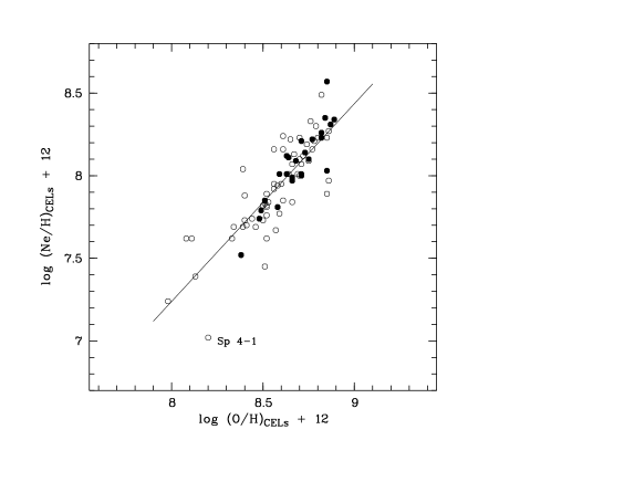
Figure 27: Neon abundances plotted against those of oxygen for GBPNe (filled circles) and GDPNe (open circles). For both elements, abundances deduced from CELs are adopted. The straight line represents a linear regression for both bulge and disk PNe.

Stanghellini et al. (2006) found an average Ne/O ratio of $0.27\pm 0.10$ for their sample of Galactic PNe. They argued that the ratio is independent of the nebular morphology and thus on stellar population. For our samples of bulge and disk PNe, we obtain an average Ne/O abundance ratio of $0.25\pm 0.08$ and $0.24\pm 0.08$, respectively, in good agreement with the result of Stanghellini et al. (2006). It is interesting that the Ne/O abundance ratios obtained for the Orion Nebula by Simpson et al. (1998) and for two H ii regions, G333.6-0.2 and W43, by Simpson et al. (2004) are also 0.25. The Ne/O abundance ratios derived from PN and H ii region observations are therefore consistently higher than the solar value of 0.15 (Lodders 2003; Asplund et al. 2005). If we accept the average Ne/O ratio of 0.25 deduced for Galactic PNe, and combine the value with the solar oxygen abundance of 8.69 from Lodders (2003), we obtain a neon abundance of 8.09, which is significantly higher than the currently recommended value of 7.87 for the Sun but is remarkably consistent with the value 8.11 deduced from solar coronal line measurements (Feldman & Widing 2003).

The relatively high neon abundance of PNe has also been observed and discussed previously. Pottasch & Beintema (1999) suggested that neon is created in NGC 6302, a bipolar PN ionized by a hidden ionizing source of probably the highest temperature known for a star ($\ga 200,000$ K). Using multi-waveband data, they deduced ionic abundances from Ne⁺ up to Ne⁵⁺ and obtained a total Ne elemental abundance of 8.34, which is 0.5 and 0.3 dex higher than the solar value and the average abundance of B-stars, respectively. Theoretically, Karakas & Lattanzio (2003) suggest that some PNe may have experienced moderate neon enrichment. The mechanism occurs for stars of initial metallicities less than 0.008 and initial masses in the range of 2–4 $M_{\odot}$, where ²²Ne is produced in sufficient quantities to affect the total neon abundance by more than 20 pet cent, about 0.08 dex. However, if the mechanism only operates in metal-poor stars in a narrow range of initial mass, then it is unlikely it will affect the average neon abundance of PNe by any significant amount. Pottasch & Bernard-Salas (2006) argued that the higher Ne/O ratio in PNe compared to the Sun is more likely caused by the destruction of oxygen in progenitor stars of PNe. Model calculations by Karakas (2003) show that some oxygen is indeed destroyed in stars more massive than 5 $M_{\odot}$ of initial metallicity $Z=0.004$ and 0.008. The process however also produce copious nitrogen, which is inconsistent with observations. On the other hand, her calculations for stars of initial metallicity $Z=0.02$ (i.e. solar composition) and of initial masses of 6 and 6.5 $M_{\odot}$, a moderate N/O ratio of about 1.2 is found, which is more compatible with observations. To explain the above the average neon abundance of PNe requires a significant fraction of PNe evolve from progenitor stars in such a restrictive range of initial mass and metallicity, an assumption that is obviously unrealistic. The average oxygen abundance deduced from CELs for the TLW disk sample of PNe is 8.60, whereas that of the WL07 bulge sample is 8.70, close to the solar value of 8.69 (c.f. Table 14). Thus depletion of oxygen in PNe is likely to be small if any, and it is unlikely that the high Ne/O ratios observed in PNe is caused by the destruction of oxygen in their progenitor stars. From the above discussion, we conclude that abundances deduced from PNe provide strong, albeit indirect, evidence that the solar neon abundance recommended by Asplund et al. (2005) may have been underestimated.

Helioseismological studies have indeed pointed to a higher solar neon abundance. As a consequence of the application of a time-dependent 3D hydrodynamical model of the solar atmosphere instead of the earlier 1D hydrodynamical model, the metal content in the solar convection zone has decreased by almost a factor of two. Amongst them, abundances of key elements such as, C, N and O have been lowered by approximately 0.2–0.3 dex from the earlier widely adopted values (see Asplund et al. 2005 for a review). Those large downward revisions however have posed serious challenges, most notably for helioseismology. Solar models which adopt the new solar abundances as input can no longer satisfactorily match helioseismological observations. On the other hand, Bahcall et al. (2005) show that raising the solar neon abundance to 8.29 (or ${\rm Ne/O}=0.42$) can in principle bring the solar model back into agreement with the helioseismological measurements. The suggestion is supported by Chandra measurements of Ne/O ratios for a sample of 21 nearby solar-like stars, yielding an error-weighted mean Ne/O ratio of 0.41 (Drake & Testa 2005). However, a reanalysis of the solar corona data by Schmelz et al. (2005) recovered the old lower solar Ne/O ratio of 0.15 (Grevesse & Sauval 1998). In a more recent study, Liefke & Schmitt (2006) derived a Ne/O ratio of $\sim 0.28$, an intermediate value for the inactive, solar-like star $\alpha$ Cen (primarily $\alpha$ Cen B, which is the dominant component in X-rays). It seems that the problem of the solar Ne/O abundance ratio and consequently the absolute abundance of Ne remains to be sorted out.

7.4 Magnesium

Table 14 shows that GBPNe have an average CEL abundance of the $\alpha$-element oxygen that is almost identical to the solar value. While for the third-row $\alpha$-element magnesium, its mean abundance deduced from ORLs, 7.71$\pm 0.06$, is about 0.15 dex higher than the solar value 7.55. The latter is almost identical to the average magnesium abundance 7.56, also derived from ORLs, for the TLW disk sample of PNe. As previously argued by Barlow et al. (2003), depletion of magnesium onto dust grains in PNe is likely to be small, probably less than 30 per cent.

The result confirms previous studies which find that that magnesium is enhanced in the Galactic bulge (, McWilliam & Rich1994). Large enhancements of $\alpha$-elements neon and magnesium are also in the peculiar bulge PN M 2-24 (, Zhang & Liu2002). In a recent abundance study of 27 RGB stars towards the Galactic bulge in Baade’s Window based on Keck/HIRES echelle observations, Fulbright et al. (2005, 2006) found enhanced [$\alpha$/Fe] ratios for all bulge giants, including those at super-solar metallicities. The enhancement of magnesium in GBPNe and the large [$\alpha$/Fe] ratios in bulge giants, combined with the old age for the bulge, point to Type II supernovae as the primary enrichment process in the bulge.

8 Conclusions

In the current work, we present careful abundance analyses for a sample of 25 GBPNe plus 6 GDPNe, using both CELs and ORLs. The results are compared to those of disk PNe published in the recent literature and to the theoretical predictions of Ma01. We find,

1. CEL abundances deduced in the current work are consistent, within 0.2 dex, with those published in the literature for samples of GBPNe, including W88 (Webster, 1988), RPDM97 (, Ratag et al.1997), SRM98 (Stasińska et al., 1998), CMKAS00 (, Cuisinier et al.2000) , ECM04 (Escudero et al., 2004) and EBW04 (Exter et al., 2004). An exception is EC01 (Escudero & Costa, 2001), which yields average abundances that are at odds with all other samples of GBPNe.

2. GBPNe are found to be slightly more metal rich on average than GDPNe, by approximately 0.1 to 0.2 dex. GBPNe also have C/O ratios systematically lower than GDPNe, by approximately 0.2 dex.

3. Bulge PNe, similar to disk PNe, also exhibit ubiquitous discrepancies between $T_{\rm e}$  and heavy element abundances derived from CELs and those deduced from CELs. The distribution of the abundance discrepancy factor, adf, for the bulge PNe are similar to that of disk PNe. Analyses also confirm many of the trends previously found for disk PNe, such as the adf is positively correlated with the difference between the [O iii] forbidden line temperatures and the H i Balmer jump temperatures, and that for a given nebula, values of adf deduced for all abundant second-row elements are comparable.

4. Based on ORL abundance analyses, we have obtained reliable C/O abundance ratios for a substantial sample of GBPNe. By comparing the observed C/O ratios with the recent theoretical predictions of Ma01, we conclude that GBPNe were probably formed in more enriched environments than disk PNe, and that Ma01 may have overestimated the carbon yield by as much as 0.4 dex. In addition, we find that GBPNe tend to have more massive progenitor stars than GDPNe do.

5. The average Ne/O ratio deduced from PNe in the WL07 and TLW samples is about 0.25, much higher than the current recommended solar value. This may points to a solar neon abundance that has been underestimated by 0.2 dex.

6. For the first time, abundances of the important $\alpha$-element magnesium have been determined using ORLs for a handful of bulge and disk PNe. We find that GBPNe have an average abundance about 0.13 dex higher than GDPNe. The latter have an average abundance almost identical to the solar value. The enhancement of magnesium in GBPNe and [$\alpha$/Fe] in bulge giants suggests that the primary enrichment process of the bulge was Type-II SNe.

9 Acknowledgments

The work is partially supported by Grant #10325312 of the National Natural Science Foundation of China. We would also like to thank Dr. R. Rubin for a critical reading of the manuscript prior to its submission.

Appendix A Line fluxes

Table 15: Ultraviolet and optical line fluxes on a scale where ${\rm H}\beta=100$. A superscript ^s denotes the emission is mainly from the central star and a ^ps indicates that stellar emission contributes at least partially the observed feature. (This is only a sample of this table: the full version is avaiable online as supplementary meterial.)

Cn 1-5
$\lambda_{\rm obs}$	$F(\lambda)$	$I(\lambda)$	Ion	$\lambda_{0}$	Mult
1246.53s	11.480	72.136	N V	1240
1345.60s	4.309	20.958	O VI	1342
1375.11s	8.256	37.868	O V	1371.29
1553.86ps	56.230	213.618	C IV	1551
1641.53ps	16.560	59.797	He II	1640
1720.70s	6.039	21.368	N IV	1718.55
1908.64	36.220	145.257	C III]	1906.68
3189.71	3.944	6.356	He I	3188.67	V3
3205.03s	2.797	4.472	He II	3203.10	3.5
3704.33	1.703	2.284	H 16	3703.86	H16
3712.44	1.338	1.792	H 15	3711.97	H15
3722.31	20.510	27.409	H 14	3721.94	H14
3727.06	58.640	78.365	[O II]	3726.03	F1
3734.84	1.747	2.329	H 13	3734.37	H13
3750.62	1.950	2.594	H 12	3750.15	H12
3770.04	2.852	3.777	H 11	3770.63	H11
3799.11	5.574	7.341	H 10	3797.90	H10
3817.55	4.134	5.420	He I	3819.62	V22
3833.94	8.317	10.867	H 9	3835.39	H9
3867.80	70.260	91.077	[Ne III]	3868.75	F1
3887.79	18.000	23.228	H 8	3889.05	H8
3966.49	23.230	29.474	[Ne III]	3967.46	F1
3968.79	11.940	15.132	H 7	3970.07	H7
4008.82	0.236	0.296	He I	4009.26	V55
4068.16	3.894	4.820	[S II]	4068.60	F1
4071.56	0.204	0.252	O II	4072.16	V10
4075.82	1.383	1.708	[S II]	4076.35	F1
4088.94	0.055	0.068	O II	4089.29	V48a
4096.90	0.559	0.687	N III	4097.33	V1
4101.27	20.530	25.210	H 6	4101.74	H6
4120.15	0.292	0.357	O II	4121.46	V19
4132.42	0.087	0.106	O II	4132.80	V19
4143.32	0.449	0.546	He I	4143.76	V53
4152.80	0.100	0.121	O II	4153.30	V19
4155.96	0.068	0.082	O II	4156.53	V19
4236.61	0.049	0.058	N II	4236.91	V48a
4241.25	0.113	0.133	N II	4241.24	V48a
4266.66	1.109	1.305	C II	4267.15	V6
4275.85	0.092	0.108	O II	4275.55	V67a
4283.94	0.049	0.058	O II	4283.73	V67c
4339.93	40.520	46.763	H 5	4340.47	H5
4349.05	0.123	0.142	O II	4349.43	V2
4362.69	3.061	3.509	[O III]	4363.21	F2
4387.39	0.719	0.819	He I	4387.93	V51
4391.59	0.043	0.049	Ne II	4391.99	V55e
4437.13	0.066	0.074	He I	4437.55	V50
4470.96	5.974	6.650	He I	4471.50	V14
4480.86	0.021	0.023	Mg II	4481.21	V4
4530.00	0.053	0.058	N III	4530.86	V3
4561.97	0.076	0.082	Mg I]	4562.60
4570.59	0.221	0.240	Mg I]	4571.10
4630.08	0.134	0.143	N II	4630.54	V5
4633.66	0.294	0.313	N III	4634.14	V2
4639.80	0.457	0.486	N III	4640.64	V2
4641.01	0.540	0.574	N III	4641.84	V2
4648.86	0.378	0.401	O II	4649.13	V1
4657.71	0.941	0.995	[Fe III]	4658.10	F3
4661.39	0.081	0.086	O II	4661.63	V1

Table 16: Infrared line fluxes of PN Cn 1-5, M 2-23 and NGC 6567.

Lines	$F(\lambda)$	$I(\lambda)$
	($10^{-12}$ ergs cm-2 s-1)	[$I({\rm H}\beta)=100$]
Cn 1-5
[O iii] $52\mu$m	21.16	343
[O iii] $88\mu$m	8.39	136
[N iii] $57\mu$m	9.66	157
[C ii] $158\mu$m	0.75	12
M 2-23
H i 6-4 $2.63\mu$m	0.75	285
H i 5-4 $4.05\mu$m	1.37	520
H i 6-5 $7.46\mu$m	0.45	171
[Ar iii] $8.99\mu$m	1.06	401
[S iv] $10.5\mu$m	2.43	923
[Ne ii] $12.8\mu$m	0.79	299
[Ne iii] $15.6\mu$m	13.8	5241
[S iii] $18.7\mu$m	0.85	324
[Ne iii] $36.0\mu$m	0.64	243
NGC 6567
H i 5-4 $4.1\mu$m	0.81	7.07
[Ar iii] $8.99\mu$m	1.08	9.39
[S iv] $10.5\mu$m	10.1	87.7
[Ne iii] $15.6\mu$m	28.9	252
[S iii] $18.7\mu$m	1.25	10.85
[Ne iii] $36.0\mu$m	2.25	19.6
[O iii] $52\mu$m	51.1	455
[O iii] $88\mu$m	29.7	264

References

- Aaquist & Kwok (1990) Aaquist O. B., Kwok S., 1990, A&AS, 84, 229
- (2) Acker A., Köppen J., Stenholm B., Raytchev B., 1991, A&AS, 89, 237
- Acker & Neiner (2003) Acker A., Neiner C., 2003, A&A, 403, 659
- Acker et al. (1992) Acker A., Ochsenbein F., Stenholm B., Tylenda R., Marcout J., Schohn C., 1992, Strasbourg - ESO catalogue of galactic planetary nebulae. Part 1; Part 2 (A92)
- Alexander & Balick (1997) Alexander J., Balick B., 1997, AJ, 114, 713
- (6) Aller L. H., Keyes C. D., 1987, ApJS, 65, 405
- Asplund et al. (2005) Asplund M., Grevesse N., Sauval A. J., 2005, in Cosmic Abundances as Records of Stellar Evolution and Nucleosynthesis, ed. T. G. Barnes III & F. N. Bash (San Francisco: ASP), ASP conf. Ser., 336, p. 25
- Bahcall et al. (2005) Bahcall J. N., Basu S., Serenelli A. M., 2005, ApJ, 631, 1281
- Barlow et al. (2003) Barlow M. J., Liu X.-W., Pequignot D., Storey P. J., Tsamis Y. G., Morisset C., 2003, in Kwok S., Dopita M., Wood P. R., eds. IAU Symp., 209, Planetary Nebulae: Their Evolution and Role in the Universe. Astrono. Soc. Pac., San Francisco, p. 373
- Bastin (2006) Bastin R. J., 2006, PhD thesis, University College London
- (11) Cahn J. H., Kaler J. B., Stanghellini L., 1992, ApJS, 94, 399 (CKS92)
- Cardelli et al. (1989) Cardelli J. A., Clayton G. C., Mathis J. S., 1989, ApJ, 345, 245 (CCM89)
- Condon & Kaplan (1998) Condon J. J., Kaplan D. L., 1998, ApJS, 117, 361
- (14) Cuisinier F., Maciel W. J., Köppen J., Acker A., Stenholm B., 2000, A&A, 353, 543 (CMKAS00)
- Davey et al. (2000) Davey A. R., Storey P. J., Kisielius R., 2000, A&AS, 142, 85
- (16) Dopita M. A., Henry J. P., Tuohy I. R., Webster B. L., Roberts E. H., Byun Y.-I., Cowie L. L., Songaila A., 1990, ApJ, 365, 640
- Drake & Testa (2005) Drake J., Testa P., 2005, Nature, 436, 525
- (18) Durand S., Acker A., Zijlstra A., 1998, A&AS, 132, 13 (D98)
- Ercolano et al. (2004) Ercolano B., Wesson R., Zhang Y., Barlow M. J., De Marco O., Rauch T., Liu X.-W., 2004, MNRAS, 354, 558
- Escudero & Costa (2001) Escudero A. V., Costa R. D. D., 2001, A&A, 380, 300 (EC01)
- Escudero et al. (2004) Escudero A. V., Costa R. D. D., Maciel W. J., 2004, A&A, 414, 211 (ECM04)
- Exter et al. (2004) Exter K. M., Barlow M. J., Walton N. A., 2004, MNRAS, 349, 1291 (EBW04)
- Feldman & Widing (2003) Feldman U., Widing K. G., 2003, Sp.Sci.Rev. 107, 665
- Fulbright et al. (2005) Fulbright J. P., Rich R. M., McWilliam A., 2005, NuPhA, 758, 197
- Fulbright et al. (2006) Fulbright J. P., McWilliam A., Rich R. M., 2006, astro-ph/0609087
- Garnett & Dinerstein (2001) Garnett D. R., Dinerstein H. L., 2001, RMxAA (Conf. Ser), 10, 13
- (27) Geisler D., Friel E., 1992, AJ, 104, 128
- (28) Górny S. K., Stasińska G., Escudero A. V., Costa R. D. D., 2004, 427, 231
- Grevesse & Sauval (1998) Grevesse N., Sauval A.J., 1998, Space Sci. Rev., 85, 161
- (30) Henry R. B. C., 1989, MNRAS, 241, 453
- Henry et al. (2004) Henry R. B. C., Kwitter K. B., Balick B., 2004, AJ, 127, 2284
- (32) Howarth I. D. 1983, MNRAS, 203, 301 (H83)
- (33) Ibata R. A., Gilmore G. F., 1995, MNRAS, 275, 605
- Iben et al. (1983) Iben I.(Jr), Kaler J. B., Truran J. W., Renzini A., 1983, ApJ, 264, 605
- Idiart et al. (1996) Idiart T. P., de Freitas Pacheco J. A., Costa R. D. D., 1996, AJ, 111, 1169
- Kaler et al. (1997) Kaler J. B., Shaw R. A., Browning L., 1997, PASP, 109, 289
- Karakas & Lattanzio (2003) Karakas A. I., Lattanzio J. C., 2003, PASA, 20, 393
- Karakas (2003) Karakas A. I., 2003, Thesis, Monash Univ. Melbourne
- (39) Kingsburgh R. L., Barlow M. J., 1994, MNRAS, 271, 257 (KB94)
- Kisielius & Storey (2002) Kisielius R., Storey P. J., 2002, A&A, 387, 1135
- (41) Kisielius R., Storey P. J., Davey A. R., Neale L. T., 1998, A&AS, 133, 257
- (42) Köppen J., Acker A., Stenholm B., 1991, A&A, 248, 197
- (43) Kwok S., 1994, PASP, 106, 344
- Leisy & Dennefeld (2006) Leisy P., Dennefeld M., 2006, A&A, 456, 451
- Lester & Dinerstein (1984) Lester D. F., Dinerstein H. L., 1984, ApJ, 281, L67
- Liefke & Schmitt (2006) Liefke C., Schmitt J. H. M. M., 2006, A&A, 458, L1
- Liu (1998) Liu X.-W., 1998, MNRAS, 295, 699
- Liu (2003) Liu X.-W., 2003, in Kwok S., Dopita M., Wood P. R., eds. IAU Symp., 209, Planetary Nebulae: Their Evolution and Role in the Universe. Astrono. Soc. Pac., San Francisco, p. 373
- Liu (2006a) Liu X.-W., 2006a, in Stanghellini L., Walsh J. R., Douglas N. G., eds. ESO Astrophysics Symposia, Planetary Nebulae beyond the Milky Way. Springer-Verlag Berlin Heidelberg, p.169
- Liu (2006b) Liu X.-W., 2006b, in Barlow M. J., Mendez R. H., eds. IAU Symp., 234, Planetary Nebulae in Our Galaxy and Beyond. Astrono. Soc. Pac., San Francisco, p.219
- Liu et al. (2006) Liu X.-W., Barlow M. J., Zhang Y., Bastin R. J., Storey P. J., 2006, MNRAS, 368, 1959
- Liu & Danziger (1993) Liu X.-W., Danziger I. J., 1993, MNRAS, 263, 256
- Liu et al. (2001) Liu X.-W., Luo S.-G., Barlow M. J., Danziger I. J., Storey P. J., 2001, MNRAS, 327, 141
- Liu et al. (1995) Liu X.-W., Storey P. J., Barlow M. J., Clegg R. E. S., 1995, MNRAS, 272, 369
- Liu et al. (2000) Liu X.-W., Storey P. J., Barlow M. J., Danziger I. J., Cohen M., Bryce M., 2000, MNRAS, 312, 585
- (56) Liu Y., Liu X.-W., Barlow M. J., Luo S.-G., 2004, MNRAS, 353, 1251 (LLBL04)
- (57) Liu Y., Liu X.-W., Luo S.-G., Barlow M. J., 2004, MNRAS, 353, 1231
- (58) Luo S.-G., Liu X.-W., Barlow M. J., 2001, MNRAS, 326, 1049
- Lodders (2003) Lodders K., 2003, ApJ, 591, 1220
- (60) Marigo P., 2001, A&A, 370, 194 (Ma01)
- (61) Massa D., Savage B., 1989, In: Louis J. A., A. G. G. M., Tielens, eds., IAU Symp., 135, Interstellar Dust, Kluwer, Dordrecht, p. 3
- (62) Mathis J. S., Torres-Peimbert S., Peimbert M., 1998, ApJ, 495, 328
- (63) McWilliam A. 1997, ARA&A, 35, 503
- (64) McWilliam A., Rich R.M., 1994, ApJS, 91, 749
- Middlemass (1990) Middlemass D., 1990, MNRAS, 244, 294
- (66) Nakasato N., Nomoto K., 2003, ApJ, 588, 842
- (67) Peimbert M., 1971, Boletin de los Observatorios Tonantzintla y Tacubaya, 6, 29
- (68) Péquignot D., Amara M., Liu X.-W., Barlow M. J., Storey P. J., Morisset C., Torres-Peimbert S., Peimbert M., 2002, RMxAA (Conf. Ser.), 12, 142
- Péquignot et al. (2003) Péquignot D., Liu X.-W., Barlow M. J., Storey P. J., Morisset C., 2003, in Kwok S., Dopita M., Wood P. R., eds. IAU Symp., 209, Planetary Nebulae: Their Evolution and Role in the Universe. Astrono. Soc. Pac., San Francisco, p.347
- Pottasch & Beintema (1999) Pottasch S. R., Beintema D.A., 1999, A&A, 347, 975
- Pottasch & Bernard-Salas (2006) Pottasch S. R., Bernard-Salas J., 2006, A&A, 457, 189
- (72) Ratag M. A., Pottasch S. R., Dennefeld M., Menzies J. W., 1992, A&A, 255, 255
- (73) Ratag M. A., Pottasch S. R., Dennefeld M., Menzies J. W., 1997, A&AS, 126, 297 (RPDM97)
- (74) Renzini A., Voli M., 1981, A&A, 94, 175
- (75) Rich R. M., 1988, AJ, 95, 828
- (76) Ruffle P. M. E., Zijlstra A. A., Walsh J. R., Gray M. D., Gesicki K., Minniti D., Comeron F., 2004, MNRAS, 353, 796
- Schmelz et al. (2005) Schmelz J. T., Nasraoui K., Roames J. K., Lippner L. A., Garst J. W., 2005, ApJ, 634, L197
- Seaton (1979) Seaton M. J., 1979, MNRAS, 187, 785
- Shen et al. (2004) Shen Z.-X., Liu X.-W., Danziger I. J., 2004, A&A, 422, 563
- Simpson et al. (2004) Simpson J. P., Rubin R. H., Colgan S. W. J., Erickson E. F., Haas, M. R., 2004, ApJ, 611, 338
- Simpson et al. (1998) Simpson J. P., Witteborn F. C., Price S. D., Cohen M., 1998, ApJ, 508, 268