Computational Coarse Graining of a
Randomly Forced 1-D Burgers Equation

Abstract

We explore a computational approach to coarse graining the evolution of the large-scale features of a randomly forced Burgers equation in one spatial dimension. The long term evolution of the solution energy spectrum appears self-similar in time. We demonstrate coarse projective integration and coarse dynamic renormalization as tools that accelerate the extraction of macroscopic information (integration in time, self-similar shapes, and nontrivial dynamic exponents) from short bursts of appropriately initialized direct simulation. These procedures solve numerically an effective evolution equation for the energy spectrum without ever deriving this equation in closed form.

I Introduction

The behavior of physical systems is frequently observed, and modeled, at different levels of complexity. Laminar Newtonian fluid flow is a case in point: it is modeled at the atomistic level through molecular dynamics simulators; at a “mesoscopic” level through Lattice Boltzmann models; and (in physical and engineering practice) through continuum macroscopic equations for density, momentum and energy: the Navier–Stokes. What makes the latter, coarse grained description possible is an appropriate closure, in this case Newton’s law of viscosity, which accurately models the effect of higher order, unmodeled quantities (such as the stresses) on the variables (“observables”) in terms of which the model is written (the velocity gradients). Such closures are often known from physical and engineering observation and practice long before their mathematical justification becomes available (in this case, through Chapman–Enskog expansions and kinetic theory). It is, of course, tempting to consider a situation in which the fine scale description is the Navier–Stokes equations themselves, and the coarse grained description is an evolution equation for some observables of turbulent velocity fields, or possibly of ensembles of such fields. Discovering the appropriate observables and deriving such evolution equations has been a long-standing ambition in both physics and mathematics. Our goal here is much more modest: we present a very simple illustration of a problem for which a fine scale description is available, and for which (based on extended observations of direct simulation) we have reason to believe that a coarse grained evolution equation exists – yet it is not available in closed form. We illustrate how (with a good guess of the appropriate coarse grained observables) we circumvent the derivation of a closed form coarse grained model, but still perform scientific computing tasks at the coarse grained level. The numerical tasks we demonstrate are coarse projective integration, which accelerate the (coarse grained) computations of the system evolution, and coarse dynamic renormalization, which (when the coarse grained evolution is self-similar, as the case appears to be here) targets the computation of the self-similar solution shape and the corresponding exponents. This is an illustration of the so-called Equation-Free framework for coarse grained scientific computation in the absence of explicit quantitative closures and the resulting coarse grained evolution equations manifesto ; pnas ; manifesto_short .

We consider the one dimensional in space, randomly forced Burgers equation,

$$\frac{\partial u}{\partial t}+\frac{1}{2}\frac{\partial u^{2}}{\partial x}=\nu_{\mbox{\small hyp}}(-1)^{n+1}\frac{\partial^{2n}u}{\partial x^{2n}}+f(x,t),$$ (1)

subject to periodic boundary conditions over the domain $x\in[0,2\pi]$. We start with random very low energy initial conditions. We are interested in the relatively long term and large scale properties of this system in the inviscid limit, when subject to a random forcing at the small scales. In order to achieve this inviscid limit numerically, we consider a general dissipation term of the form $\nu_{\mbox{hyp}}\,(-1)^{n+1}\partial^{2n}u/\partial{x}^{2n}$ following chekhlov95 . The coefficients $\nu_{\mbox{hyp}}$ and $n$ are chosen so that the dissipation acts only at the highest wavenumbers; here, their values are $\nu_{\mbox{hyp}}=10^{-54}$ and $n=7$. This choice of dissipation is based on the assumption that the universal ranges of the system are not sensitive to a particular choice of the parameters $\nu_{\mbox{hyp}}$ and $n$ chekhlov95 . The white–in–time random force $f(x,t)$ is defined in Fourier space by

$$\overline{f(k,\omega)f(k^{\prime},\omega^{\prime})}={\cal P}\exp\Big{[}-\frac{(k-k_{s})^{2}}{\sigma_{f}^{2}}\Big{]}\delta(k-k^{\prime})\delta(\omega-\omega^{\prime}),\qquad\mbox{with }{\cal P}=\frac{f_{0}^{2}}{2\pi\sigma_{f}^{2}},$$ (2)

where $k$ and $\omega$ are the spatial and temporal frequencies. The forcing term has a peak at wavenumber $k=k_{s}=1000$ and dies off at large wavenumbers; the dissipation term is essentially zero up to around wavenumber $k=3000$ and only becomes important at much larger wavenumbers; see Fig. 1.

\psfrag{k}{$k$}\psfrag{forcing}{\small forcing}\psfrag{dissipation}{\small dissipation}\includegraphics[scale={0.4}]{epsfiles/force_dissp.eps}

Figure 1: Forcing amplitude $\frac{f_{0}^{2}}{2\pi\sigma_{f}}\exp[-\frac{(k-k_{s})^{2}}{\sigma_{f}^{2}}]$ and dissipation term $\nu_{\mbox{hyp}}k^{2n}$.

Before we start our computations, we briefly recall certain known features of the equations and their dynamics. It is quite remarkable that equations (1,2) have non-trivial asymptotic behavior in both the ultraviolet (UV, $k>k_{s}$) and the infrared (IR, $k<k_{s}$) limits. Attempts to use (1,2) as a simplified 1–D model for the investigation of small scale features of 3–D turbulence, aimed at recovering $E(k)\propto k^{-5/3}$ in the small scale limit, were based on deep similarities between the two: the total energy in this system is $\overline{u^{2}}/2\equiv K\approx({\cal P}L)^{2/3}$ and, as in 3–D turbulence, the inertial range $k_{s}\ll k\ll k_{d}$ where $k_{d}$ is the dissipation wave number, is characterized by a constant energy flux $J_{E}={\cal P}$, which, in the interval $r\ll L=1/k_{s}$, is reflected in the analytic behavior of the third-order structure function

$$S_{3}(r)=\overline{(\delta_{r}u)^{3}}\equiv\overline{(u(x+r)-u(x))^{3}}=-12{\cal P}r.$$ (3)

Even in decaying high Re–turbulence this equation is correct: $\partial E/\partial t$ is very small. At first glance, due to the shock formation leading to the $E(k)\propto k^{-2}$ energy spectrum (rather than $E(k)\propto k^{-x}$ with the exponent $x\approx 5/3$), these attempts failed. However, the model revealed a non-trivial bi-scaling behavior of the structure functions $S_{n}(r)=\overline{(u(x+r)-u(x))^{n}}\propto r^{n}$ for $n\leq 1$ and $S_{n}(r)\propto r$ for $n\geq 1$ frisch . The model also generated asymmetric probability densities with algebraically decaying tails $P(\delta_{r}u)$ for large amplitude fluctuations $\delta_{r}u<0$ chekhlov95 ; vyPRL96 . The properties of this tail attracted the attention of various groups and are reasonably well understood in terms of the dissipation anomaly introduced by polyakov95 ; they have also been analytically obtained in e97 ; e99 ; bec00 . The Burgers equation stirred by a force with the $k^{-1}$ spectrum does lead to the logarithmically corrected Kolmogorov energy spectrum discovered in chekhlov95b and does not have multifractality mitraArXiv .

The IR properties of (1,2) in the range $k\ll k_{s}$, on which we focus in this paper, are also quite interesting and non-trivial. It was determined, on the basis of the one-loop calculation (also numerically verified in vyPRL88 ) that in the limit $k\ll k_{s}$, (1,2) is equivalent to the Burgers equation driven by a random force with $\overline{f(k)^{2}}\propto k^{2}$–spectral density, which is called the KPZ equation, governing various interfacial phenomena kpz . The renormalization group methodology applied to the KPZ equation forster77 led to the equilibrium energy spectrum $E(k)\propto k^{D-1}=\mbox{const}$ (here $D=1$) and to a non-Gaussian dynamic fixed point with non-trivial dynamic scaling exponents,

$$\omega\propto k^{\frac{3}{2}},$$ (4)

indicating strongly non-diffusive behavior: $r(t)\propto t^{\frac{3}{2}}$. These predictions, including dynamic scaling, have been numerically verified in vyPRL88 . Numerical simulations in the IR range become progressively slower; our computer-assisted approach aims at accelerating such simulations (see also kesslerPRE ).

Our numerical simulator integrates equation (1) in time using a pseudo-spectral scheme with a $N=22000$ Fourier mode spatial discretization. Thus, the smallest scale resolved by our simulator is $\Delta x=\pi/N=1.428\times 10^{-4}$. The nonlinear term is computed using the fast Fourier transform. The temporal discretization treats the linear term exactly and uses a third order Runge–Kutta–Wray scheme for the nonlinear term. The random forcing term in Fourier space is $f(k,t)=\sqrt{{\cal P}/\Delta t}\sigma_{k}$, where $\sigma_{k}$ is a random number generated from a Gaussian distribution with zero mean and unit standard deviation, and $\Delta t$ is the time step of integration. The various parameters chosen are $\Delta t=5\times 10^{-6}$, $f_{0}=5\times 10^{2}$, $k_{s}=1000$, $\sigma_{f}=250$, $\nu_{\mbox{hyp}}=10^{-54}$, and $n=7$. An ensemble of 16 distinct realizations was computed, and the results averaged to achieve good statistics.

We begin by observing direct numerical simulations of the evolution of equation (1) over time. Fig. 2 shows such a transient, starting from the zero initial condition, $u(k,t=0)=0$, for all $k$. The energy spectra $E(k,t)$ are plotted after $1000$, $5000$, $25000$, and $300000$ time steps; the insets show the corresponding 1D velocity fields. Visually, we can discern no clear trend in the evolution of the velocity fields themselves, which appear random; yet, we easily see a definite smooth structure in the evolution of the energy spectrum.

For $k\geq 700$, the spectrum seems to quickly achieve a steady state profile within less than 1000 time steps: the energy provided by the noise is balanced by the strong dissipation at high wavenumbers. It is much more interesting to observe $E(k)$ for $1\leq k\leq 500$; here the spectrum quickly acquires a “corner-like” shape which appears to evolve smoothly in time, and moves towards lower wavenumbers while maintaining this shape. This “traveling front-like” evolution progressively slows down as the “corner” evolves towards lower wavenumbers.

\psfrag{a}{(a)}\psfrag{b}{(b)}\psfrag{c}{(c)}\psfrag{d}{(d)}\psfrag{e}{$E(k)$}\psfrag{k}{$k$}\psfrag{g}{$k_{f}$}\includegraphics[scale={0.75}]{epsfiles/spec_field_evl1.eps}

Figure 2: Evolution of $E(k)$ from the zero initial condition $u(k,0)=0$, for all $k$. The spectra are shown after 1000, 5000, 25000, and 300000 time steps, with time increasing in the direction of the arrow. The velocity fields corresponding to the spectra are shown in the insets, in the same color as the spectra.

Theoretical considerations forster77 ; vyPRL88 indicate that in the range $k<k_{s}$, the evolving energy spectrum $E(k)$ consists of three regimes. For $k=O(k_{s})$, the spectrum is not universal and depends on the properties of the forcing function. For $1/L\ll k_{I}(t)\ll k\ll k_{s}$, $E(k)=k^{D-1}=\mbox{const}$ (here $D=1$); and in the time-dependent large-scale limit $1/L\ll k<k_{I}(t)$, the energy spectrum is given by a universal relation $E(k)\propto k^{D-1+2}\propto k^{2}$, which we observe in our simulations. Superficially, the temporal evolution we observe resembles the time-dependence of a two dimensional flow driven by a small ($k_{s}=O(1)$) random force, eventually leading to the energy spectrum piling up on the smallest (integral) wave number $k_{i}=\pi/L$ and leading to the IR asymptotics $E(k)\propto k^{-3}$. We stress that the situation we are interested in may be quite different: in 2D, due to enstrophy conservation in the infrared range ($k<k_{s}$), there exists a constant, nonzero, energy flux toward large scales, leading to the so called “inverse cascade”. The third-order structure function in a 2D flow is $S_{3}=\frac{3}{2}{\cal P}r\neq 0$. In the one dimensional flow we are interested in here, the large scale thermodynamic equilibrium is flux-free and $S_{3}$ must be equal to zero, provided the system is large enough, that is, $k_{I}/k_{s}\ll 1$.

We do not work at this very long time regime; we rather observe the evolution at times intermediate between this regime and the (relatively) short time it takes for the spectrum to stabilize for $k>700$. This is the regime in which smooth and, as we argue below, apparently self-similar evolution of the energy spectrum prevails.

Based on the study of many transients like those in Fig. 2, we decided to observe the system dynamics in terms of the energy spectrum $E(k,t)$ only, which is defined as

$$E(k,t)=\left\langle\hat{u}(k,t)\hat{u}^{\ast}(k,t)\right\rangle,$$ (5)

where $\hat{u}(k,t)$ is the spatial Fourier transform of the velocity field $u(x,t)$, and $\left\langle\cdot\right\rangle$ denotes an ensemble average (here over the 16 realizations). A formal diagrammatic expansion for the evolution of the energy spectrum corresponding to (1,2) can be developed wyld61 . In the limit $k\rightarrow 0$, taking into account that all odd-order correlation functions rapidly tend to zero, the solution can be accurately represented in terms of an infinite series involving complicated integral expressions with kernels which are convolutions of the energy spectrum $E(k)$ only. Based on this, we assume that an evolution equation of the general form

$$\frac{\partial E(k,t)}{\partial t}=\mathcal{L}[E(k,t)]$$ (6)

exists and closes for the (ensemble averaged) $E(k,t)$. We do not know the nature of the operator $\mathcal{L}$ – it may not be local (in $k$–space), and the equation may not be a partial differential equation – yet the implication is that knowing $E(k,0)$ is enough to predict the (realization ensemble averaged) $E(k,t)$ for later times. If an evolution equation closes with respect to the expected spectrum only, then the remaining degrees of freedom (the phases of the velocity field Fourier coefficients) do not explicitly appear in this equation. This implies that either these variables do not couple to the spectrum evolution, or that their expected dynamics become quickly slaved to the spectrum evolution (with a relaxation time that is small compared to the spectrum evolution time scales). We test this latter ansatz by observing the solution ensemble not only through the spectrum $E(k,t)$ but also through the evolving third order structure function

$$S_{3}(r,t)=\left\langle\overline{(u(x,t)-u(x+r,t))^{3}}\right\rangle.$$ (7)

(a)                                                                    (b)

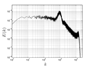
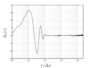
Figure 3: Long term solution, after $1.25\times 10^{6}$ time steps (a) $E(k)$ vs. $k$; (b) $S_{3}(r)$ vs. $r/\Delta x$, where $\Delta x=\pi/N$ is the smallest scale resolved in our simulations.

For completeness, the “extremely long term” steady state of $E(k,t)$ and $S_{3}(r,t)$, obtained after integrating for $1.25\times 10^{6}$ time steps is included in Fig. 3. Fig. 3(a) suggests that $E(k)$ reaches a constant value of $2\times 10^{-4}$ in the range $1\leq k\leq 150$. The structure function $S_{3}(r)$, plotted in Fig. 3(b), is practically zero in the range $200\Delta x\leq r\leq 2\pi$. The steady state value of $S_{3}(r)$ is nonzero for $r<200\Delta x$, due to the force acting primarily at small scales (corresponding to $k=1000$) and strong dissipation at the smallest scales.

The remainder of the paper is organized as follows: In Section II we discuss simulations suggesting an apparent dynamic self-similarity in the intermediate-time evolution of the spectrum. Section III briefly outlines equation free computational techniques, and demonstrates coarse projective integration of the unavailable equation for the expected spectrum evolution. Section IV then shows how to implement a dynamic renormalization fixed point algorithm that converges on the self-similar shape and pinpoints the temporal similarity exponent of its evolution. We conclude with a brief discussion.

II Apparent Dynamic Self-similarity

Here we argue that the transient evolution of $E(k)$ exhibits dynamic self-similarity. Fig. 4 clearly shows that the qualitative shape of the spectrum in the region $1\leq k\leq 500$ remains effectively unchanged, while gradually “travelling” to the left, slowly filling up the lower wavenumbers. We make this observation more precise as follows: We define a “fulcrum point” $k=k_{f}$ as the leftmost end of the apparently steady region of $E(k)$; here $k_{f}\approx 450$. As shown in Fig. 4(a), we draw straight line segments of various slopes $m_{j}$ (logarithmic in $E$ as well as in $k$) starting at the fulcrum and intersecting successive computed spectra. Let $d_{m_{j}}(t)$ be the distance of the point of intersection of each such line with the spectrum at time $t$. Our ansatz is that the distance $d_{m_{j}}(t)$ becomes uniformly stretched in (logarithmic) time. This is tested as follows: let the stretching factor along a line of slope $m_{j}$ be $r_{m_{j}}(t)=d_{m_{j}}(t)/d_{m_{j}}(t_{1})$, where $t_{1}$ is a reference time. Fig. 4(b) is a plot of $r_{m_{j}}$ versus $m_{j}$ at various times in the order listed in the figure caption; it strongly suggests that the spectrum gets stretched by the same amount along its entire profile (notice that no intersections arise with $m_{j}\lesssim-0.1$). Fig. 4(c) shows the time evolution of the stretching factor $r(t)$ (averaged over the lines of different slopes), clearly showing linearity in logarithmic time. Thus, the transient evolution of $E(k)$ appears dynamically self-similar: the spectrum in the wavenumber region $1\leq k\lesssim 450$ becomes uniformly stretched in logarithmic time, while maintaining its shape. We take advantage of this information in speeding up computations in the next section.

(a)                                         (b)                                         (c)

\psfrag{a}{$d_{m}(t_{1})$}\psfrag{b}{$d_{m}(t_{n})$}\psfrag{c}{fulcrum}\psfrag{d}{line of slope $m$}\psfrag{e}{$\log\,E(k)$}\psfrag{f}{(a)}\psfrag{g}{$k_{f}$}\psfrag{i}{{\small slope = 0.48}}\psfrag{k}{$\log\,k$}\psfrag{p}{{\small slope}, $m$}\psfrag{q}{ {\em\small t}}\psfrag{r}{{\small mean stretch}}\psfrag{t}{$\log t$}\psfrag{u}{{\small stretch}, $r_{m}$}\psfrag{y}{(b)}\psfrag{z}{(c)}\includegraphics[scale={0.35}]{epsfiles/cartoon1c.eps}

\psfrag{a}{$d_{m}(t_{1})$}\psfrag{b}{$d_{m}(t_{n})$}\psfrag{c}{fulcrum}\psfrag{d}{line of slope $m$}\psfrag{e}{$\log\,E(k)$}\psfrag{f}{(a)}\psfrag{g}{$k_{f}$}\psfrag{i}{{\small slope = 0.48}}\psfrag{k}{$\log\,k$}\psfrag{p}{{\small slope}, $m$}\psfrag{q}{ {\em\small t}}\psfrag{r}{{\small mean stretch}}\psfrag{t}{$\log t$}\psfrag{u}{{\small stretch}, $r_{m}$}\psfrag{y}{(b)}\psfrag{z}{(c)}\includegraphics[scale={0.35}]{epsfiles/strch1b.eps}

\psfrag{a}{$d_{m}(t_{1})$}\psfrag{b}{$d_{m}(t_{n})$}\psfrag{c}{fulcrum}\psfrag{d}{line of slope $m$}\psfrag{e}{$\log\,E(k)$}\psfrag{f}{(a)}\psfrag{g}{$k_{f}$}\psfrag{i}{{\small slope = 0.48}}\psfrag{k}{$\log\,k$}\psfrag{p}{{\small slope}, $m$}\psfrag{q}{ {\em\small t}}\psfrag{r}{{\small mean stretch}}\psfrag{t}{$\log t$}\psfrag{u}{{\small stretch}, $r_{m}$}\psfrag{y}{(b)}\psfrag{z}{(c)}\includegraphics[scale={0.35}]{epsfiles/meanstrch1b.eps}

Figure 4: (a) Schematic diagram showing calculation of the stretching factor. For a line of slope $m$, $r_{m}(t_{n})=d_{m}(t_{n})/d_{m}(t_{1})$. (b) Stretching factor $r_{m}(t_{i})$ vs. slope $m$ after $7,10,25,50,100,\mbox{ and }300\,(\times 1000)$ time steps; the direction of time is indicated by the arrow. Stretching is measured with respect to the spectrum at $t=2500\Delta t$. (c) Mean stretch $r(t)$ vs. $\log(t/\Delta t)$ (solid line) and a least squares fit (dotted line).

III Coarse Projective Integration

Based on our simulation observations above, we now hypothesize that an evolution equation exists and closes at the level of the energy spectrum $E(k,t)$ averaged over our ensemble of realizations. If this equation were explicitly available, a typical numerical integration scheme would start by discretizing it in $k$ (for example through finite differences, FD, or finite elements, FE) and then proceed to the derivation of ordinary differential equations (ODEs) in time for the vector of values ${\bf a}$ at the FD discretization points, or of the FE coefficients. These ODEs would be of the general form $d{\bf a}/dt={\bf F}({\bf a})$; the temporal evolution would be obtained using established numerical integration techniques, of which the simplest is arguably the explicit forward Euler method

$${\bf a}(t_{0}+\Delta t)={\bf a}(t_{0})+\Delta t\,{\bf F}({\bf a}(t_{0})).$$ (8)

Clearly, implementing this, as well as other initial value solvers, requires an evaluation of the time derivative (the right hand side of the ODE set) at prescribed system states. In projective integration gk1 ; gk2 this time derivative is not obtained through such a function evaluation of ${\bf F}({\bf a})$, since ${\bf F}({\bf a})$ is not available in closed form; instead, it is obtained from processing the results of short bursts of simulation: starting at time $t_{0}$, we integrate the original equation for a short time with a time step $\delta t\ll\Delta t$ to obtain a sequence ${\bf a}(t_{0}),{\bf a}(t_{0}+\delta t),{\bf a}(t_{0}+2\delta t),\,\ldots,\,{\bf a}(t_{0}+n\delta t)$, where $n\delta t<\Delta t$. We can then use, for example, the last two points of this sequence to estimate the time derivative, and predict ${\bf a}(t_{0}+\Delta t)$ as

$${\bf a}(t_{0}+\Delta t)\approx{\bf a}(t_{0}+(n-1)\delta t)+\frac{\Delta t-(n-1)\delta t}{\delta t}\big{(}{\bf a}(t_{0}+n\delta t)-{\bf a}(t_{0}+(n-1)\delta t)\big{)};$$ (9)

better estimators (least squares, maximum likelihood) of the time deerivative can clearly be used as well. The procedure provides an approximation of the “projected in time” state ${\bf a}(t_{0}+\Delta t)$, which can then be used to restart the computation, and the process repeats.

When the only available tool is a “black box” simulator of the system evolution equation, projective integration may significantly accelerate computations for systems with gaps in their eigenvalue spectra (separation of time scales). However, in our case, the equation we want to projectively integrate is an equation for energy spectrum evolution, while the available simulator is a simulator for velocity fields; we want to projectively integrate the coarse grained behavior (spectra) through observations of the fine scale behavior (velocities). This now becomes coarse projective integration. From our simulation we have available the full state (the velocity field ensembles) at time $t_{0}$; full direct simulation will then provide full states at each of the intermediate time steps. We restrict the full state to the coarse observables (the discretization of the spectrum); we use these observations to estimate the time derivative of these coarse observables; and we finally pass the time derivative estimates to our integrator of choice (here a simple forward Euler) in order to produce our approximation of the coarse observables at the next (projected) point in time $t_{0}+\Delta t$.

Here comes a vital step in our equation-free coarse graining approach: our “black box” simulator requires a fine scale initialization (detailed velocities); yet we only have coarse grained initial conditions (ensemble-averaged spectrum discretizations). For the procedure to continue, we need to somehow construct full fine-scale states consistent with the desired coarse initial conditions. This construction is the so-called lifting step pnas ; gkt02 ; manifesto ; manifesto_short . The missing degrees of freedom in our construction are the phases of the velocity fields. Our assumption that an equation exists and closes in terms of only ensemble averaged spectra implies that these remaining degrees of freedom either do not couple with the evolution of the coarse grained variables we retain, or, if they do (as we expect), they quickly get slaved to the coarse variables. “Quickly” here implies a comparison with the time scales of the evolution of the retained coarse variables themselves. Exploiting this “quick slaving” (which is implicit in the assumption that an equation for the retained coarse variables exists and closes) is the main point of equation-free computation: since the fine scale code is available, running it for a short time, even with wrongly initialized “additional variables”, should provide the required slaving on demand. This can be considered a subcase of optimal prediction chorin . Given an energy spectrum initial condition, we therefore initialize the velocity fields as follows: the amplitudes of the velocity Fourier modes are chosen consistently with the prescribed initial energy spectrum, while the phases are chosen randomly. We then let our direct simulator evolve for some initial “healing” interval (described below) before we start observing the solution energy spectrum, in order to estimate its time derivative; this initial period is allowed so that our “wrong” phase initialization becomes “healed”, that is, so that our phases or their statistics become slaved to the evolution of the spectra. We monitor this slaving through observations of the structure function $S_{3}(r,t)$ defined earlier.

Here is a concise description of our coarse (spectrum level) projective (forward Euler) integration. The procedure starts after we have already simulated (starting with zero initial conditions) for a period of approximately 3000 time steps; during this period the “high–$k$” end of the spectrum $E(k>k_{f})$ approaches stationarity.

1. Starting with a “current” velocity field initial condition, we evolve the randomly forced Burgers simulator for a short interval $T$, and restrict the velocity fields at successive instances within this interval to ensemble-averaged energy spectra. Fig. 5(a) shows the restricted spectra at times $t/\Delta t=$ 3500, 4500, 5500, and 7000.

2. Using the procedure described in section II, we compute the stretching factors $r_{m_{j}}(t)$ along various straight lines passing through the fulcrum and intersecting these spectra. Our discretization of the spectrum does not come in the form $E(k_{i})$ for a number of mesh points $k_{i}$ (or $\log k_{i}$), but rather in the form $(E(m_{j}),\,k(m_{j}))$ for a number of “discretization slopes” $m_{j}$; the ensemble-averaged spectrum evolution appears smooth enough, so that approximately 20 such discretization angles and simple interpolation is sufficient. We now compute the rate of change of the stretching factors in logarithmic time, and use the same to project the energy spectrum to a future time $\gg T$. Here, the stretching factors $r_{m_{j}}$ are computed along straight lines of slopes $-0.2<m_{j}<0.1$, and their rate of change in logarithmic time is computed using a least squares fit as

   $$r_{m_{j}}(t)\approx P_{1}^{m_{j}}+P_{2}^{m_{j}}\log t,$$ (10)

   where $P_{1}^{m_{j}}$ and $P_{2}^{m_{j}}$ are the coefficients of the least squares fit. We then use equation (10) to project the stretching factor to a time $t^{\ast}\gg T$, and compute the projected spectrum using

   $$\log[E(m_{j},\,t^{\ast})] =r_{m_{j}}(t^{\ast})\log[E(m_{j},\,t_{1})],$$

   $$\mbox{and}\quad\log[k(m_{j},\,t^{\ast})] =r_{m_{j}}(t^{\ast})\log[k(m_{j},\,t_{1})].$$ (11)

   An estimate of the spectrum at $t^{\ast}=30000\Delta t$ using those at times $t/\Delta t=$ 3500, 4500, 5500, and 7000 is shown in Fig. 5(a).

3. We now lift the projected spectrum to an ensemble of consistent velocity fields in order to repeat the process. This is done by randomizing the phases for all the wavenumbers, while retaining the amplitudes corresponding to the projected spectrum. More precisely, we generate 16 different initial velocity fields as $u(k,t)=\sqrt{E(k,t)}\exp(i\phi_{k})$, where $\phi_{k}$ is a random number between $0$ and $2\pi$ chosen from a uniform distribution.

4. We now repeat the process: we evolve the fine scale simulator (the randomly forced Burgers) with the initial conditions thus obtained; but before we start using the resulting spectra to estimate a new coarse time derivative and make a new forward Euler projection, we test the slaving of the injected degrees of freedom (the random phases) to our coarse observables (the spectrum). This slaving is monitored through the evolution of the newly initialized structure function $S_{3}(r)$. Fig. 5(b) shows the structure function from a simulation that has been running for some time; if we restrict to energy spectra, and then randomize the phases (that is, lift back to velocity fields) this phase information is lost. When we restart the simulation from the lifted velocity fields, however, we clearly observe that the phases “heal”, that is, $S_{3}$ acquires its original shape quickly compared to the evolution time scales of the spectrum (in less than 500 time steps, which is much smaller than the projection horizon of $>20000$ time steps). We continue now the “short burst” of fine scale simulation to collect data (restrictions to spectra) for the next projection step; the procedure (steps 1–3) then repeats.

(a)                                                                    (b)

\psfrag{z}{\small$t=30000$}\psfrag{r}{$r$}\psfrag{S3(r)}{$S_{3}(r)$}\psfrag{log(k)}{$\log k$}\psfrag{log[E(k)]}{$\log E(k)$}\psfrag{t=30400}{$t=30400$}\includegraphics[scale={0.5}]{epsfiles/proj_intc.eps}

\psfrag{z}{\small$t=30000$}\psfrag{r}{$r$}\psfrag{S3(r)}{$S_{3}(r)$}\psfrag{log(k)}{$\log k$}\psfrag{log[E(k)]}{$\log E(k)$}\psfrag{t=30400}{$t=30400$}\includegraphics[scale={0.5}]{epsfiles/s3enslavc.eps}

Figure 5: (a) Coarse projective integration and its comparison with the original direct simulation (spectra from the continuing original simulation are shown in blue). The phases of all the modes are randomized after projection. (b) Healing of $S_{3}(r)$ (black) in 400 time steps. After randomizing the phases at $t=30000\Delta t$ (flat line), their transient recovery is depicted after time steps 10, 20, 30, 40, 50, and 400. Also shown is a comparison with the original simulation at $t=30400$ (blue).

Fig. 5 shows an instantiation of such a coarse projective step. The restriction of an initial simulation used to estimate the coarse time derivative are obtained at $t/\Delta t=$ 3500, 4500, 5500, and 7000; the projection step (which here is performed in logarithmic time) brings us to $t=30000\Delta t$; the projected spectrum (black dashed line) is compared to the result of continuing the full simulation until time $t=30000\Delta t$ (blue). More importantly, the result of lifting from the projected spectrum and continuing the evolution till $t=70000\Delta t$ (black dashed line) is also seen to coincide with the result of a full simulation till $t=70000\Delta t$ (blue). Also, the computational savings in the first step of coarse projective integration can now be quantified. Using coarse projective integration, the randomly forced Burgers equation is simulated for 7000 time steps and then a projection step is used to obtain the spectrum at $t=30000\Delta t$, thus resulting in a saving of 23000 time steps, or a speedup factor of 4.3. The factor is actually a little lower because of the computational effort required for the projection step. Since the dynamics evolve in logarithmic time, this factor will increase for the later projective integration steps.

The choice of performing projective integration (in effect, Taylor series expansion of the coarse solution in the independent variable) in logarithmic rather than linear time is motivated by the observation that our transient is close to a dynamically self-similar solution. A detailed discussion of the usefulness of of (coarse) projective integration in problems with continuous symmetries, such as scale invariance, having (possible approximately) self-similar solutions can be found in mihalis .

IV Coarse Dynamic Renormalization

Direct simulations starting at $E(k)=0$ showed that the spectrum quickly evolves to a “steady state” for $k>k_{f}\approx 450$; after this initial period, its low wavenumber portion acquires a “constant shape” which is then observed, over time, to stretch gradually and rather smoothly towards $k=0$. This stretching becomes increasingly slower in linear time. In what follows we do not concern ourselves with the very fast initial transient (the establishment of a steady state for $k>k_{f}$); nor will we study the very long term dynamics that occur when the “corner” of the spectrum finally approaches $k=0$. We focus on the “intermediate time” regime during which the $k<k_{f}$ spectrum acquires its “constant shape” which then appears to travel (in logarithmic $k$ and logarithmic time) towards $k=0$. This latter observation suggests an even simpler caricature of the self-similar evolution; see Fig. 6(a): the spectrum to the left of $k_{f}$ acquires quickly the appropriate “corner like” shape, which we approximate by two straight lines meeting at a point with wavenumber $k_{0}(t)$. The energy of the wavenumbers to the right of $k_{0}$ remains more or less unchanged, anchored at the fulcrum point. The portion of the spectrum to the left of $k_{0}(t)$ subsequently simply moves towards lower $k$ with constant shape. A constant shift of this part of the spectrum in $\log k$ corresponds to a stretching by a constant factor in $k$, and clearly suggests that for our apparently self-similar solution

$$E(k,t)=E\Big{(}k\big{(}t+t_{0}\big{)}^{\beta}\Big{)},\qquad\mbox{for}\quad k<k_{0}(t),$$ (12)

and an appropriate choice of constants $\beta$ and $t_{0}$. For the data shown in Fig. 4, initialized with a zero spectrum at $t=0$ and taken at times $t\geq 125\Delta t$, the values of the exponent and the constant $t_{0}$ are computationally found to be $\beta\approx 0.633$ and $t_{0}\approx-98\Delta t$. These values can be extracted from Fig. 6(b), which shows plots of the wavenumbers $k_{0}(t)$ versus $t/\Delta t$ and $k_{0}(t)$ versus $(t+t_{0})/\Delta t$ on a logarithmic scale.

(a)                                                              (b)

\psfrag{d}{\small fulcrum}\psfrag{a}{$k_{f}$}\psfrag{n}{\small$k_{0}(t_{i})$}\psfrag{m}{\small$k_{0}(t_{0})$}\psfrag{k}{$\log k$}\psfrag{e}{$\log E(k)$}\psfrag{t}{$t/\Delta t,\,(t+t_{0})/\Delta t$}\psfrag{y}{$k_{0}$}\includegraphics[scale={0.37}]{epsfiles/selfsim_exp2.eps}

\psfrag{d}{\small fulcrum}\psfrag{a}{$k_{f}$}\psfrag{n}{\small$k_{0}(t_{i})$}\psfrag{m}{\small$k_{0}(t_{0})$}\psfrag{k}{$\log k$}\psfrag{e}{$\log E(k)$}\psfrag{t}{$t/\Delta t,\,(t+t_{0})/\Delta t$}\psfrag{y}{$k_{0}$}\includegraphics[scale={0.28}]{epsfiles/kfit3.eps}

Figure 6: (a) A cartoon illustrating the approximations to the spectra used to compute the self-similar solution. The plot shows spectra at a few select time instances. Their straight line approximations used to compute the exponents are shown in red. (b) Wavenumbers at the intersections of the spectra with the dotted green line are used to fit the constants $\beta$ and $t_{0}$ (see text). A plot of these wavenumbers $k_{0}$ vs. $t/\Delta t$ is shown (red, $\circ$), with a least squares fit of the form $k_{0}(t)=k_{\mbox{const}}(t+t_{0})^{\beta}$ (black, $\square$). Also shown are plots of $k_{0}$ vs. $(t+t_{0})/\Delta t$ (blue, $\triangledown$) and the corresponding least squares fit (black, +).

This appears consistent with the numerical simulations of Yakhot and She vyPRL88 as well as with dynamic renormalization group results suggesting a non-trivial dynamic scaling of the temporal frequency $\omega=O(k^{3/2})$ (or $kt^{2/3}\approx\mbox{const}$) as opposed to $\omega\propto\nu k^{2}$ or $k=O(\omega^{1/2})$. The same exponent is obtained using different spectrum “caricatures” based on the same low-wavenumber straight-line approximations (not shown here). We would like to stress that computation of dynamic scaling exponents is an extremely difficult and computationally expensive task. The fact that the non-trivial exponent (4) emerged from our relatively fast calculation seems remarkable. Moreover, it serves as an independent test of our coarse graining procedure.

Given these observations, it is clear that the intermediate time behavior can be recovered in an even more economical fashion than coarse projective integration: it is enough to find the “right shape” (the slope of the leftmost part of the spectrum) as well as the correct stretching rate (encoded in the exponent); this information suffices to approximate the spectra at all intermediate times. This is analogous to computing the shape and the (constant) speed of a traveling wave in a problem with translational invariance. Knowing the shape and speed we can construct the solution at any future time; scale invariance here takes the place of translational invariance for traveling, and the stretching rate (quantified by the similarity exponents) is analogous to the traveling speed. The problem therefore reduces to finding the “right” spectrum shape (for $k<k_{f}$): a spectrum $E(k,t_{1})$ which, when evolved for some time $T$ to $E(k,t_{1}+T)$ and rescaled in $k$–space, remains unchanged. This gives rise to the fixed point problem:

$$E(k,\,t_{1})-E\Big{(}k\Big{(}\frac{t_{1}+T+t_{0}}{t_{1}+t_{0}}\Big{)}^{\beta},\,t_{1}+T\Big{)}=0.$$ (13)

Solving such coarse fixed point problems using coarse time steppers has been discussed and illustrated in several contexts chenJNNFM ; zouPRE ; chenPRE ; kesslerPRE . The simplest fixed point algorithm is successive substitution: we start with an initial guess of the self-similar spectrum shape which we evolve for some time using the direct randomly forced Burgers simulator, including ensemble averaging. We then rescale the resulting spectrum by a constant factor, and repeat the process; for a discussion of a so-called template based approach to choosing the appropriate scaling factor at each iteration, see aronson01 ; rowley03 , and our choice for this problem will be discussed below. If the self-similar spectrum is stable (as is the case here), this iteration converges to its scale-invariant shape. We remark, before proceeding, that other fixed point algorithms (in particular, matrix-free Newton–Krylov–GMRES, kelley04 ) have been used for solving this type of problem; such Newton–based algorithms can converge to self-similar solutions even if they are not stable. In what follows, we demonstrate that successive substitution using a dynamically rescaled coarse time stepper does indeed converge to the right (invariant) spectrum shape.

Long direct simulation will also eventually converge to this invariant shape; yet, while approaching the right shape, the transient will also move towards lower wavenumbers (will “stretch”) and this makes the evolution increasingly slower. We therefore have the potential to realize a computational advantage by rescaling the spectrum after partial evolution to a constant reference scale, a scale in whose neighborhood the dynamics are as fast as possible in physical time; this allows us to observe the approach to the stable invariant shape without this shape stretching.

We now consider another caricature of the (ensemble averaged) spectra during our intermediate–time simulation, approximated by two straight lines in the region $k<k_{f}$ as shown in Fig. 7(a). These two straight lines intersect at a “corner”; we call this corner wavenumber $k=k_{c}$. As we discussed earlier in this section, we observe that the slope of the straight line approximating the region of the spectrum to the left of the corner remains (approximately) constant ($m=m_{\mbox{left}}$) during self-similar evolution; finding the right shape becomes then equivalent to finding this slope. In order to obtain the self-similar shape, we initialize our spectrum as follows: The portion of the spectrum to the right of the fulcrum $E(k>k_{f})$ is initialized at its (already) steady shape. For $k_{c}<k<k_{f}$, a straight line approximation is used, the slope of which is computed by a local fitting to the spectrum obtained from the initial direct simulation. Finally, for the region $k<k_{c}$, we initialize the spectrum with a straight line of a “guess” slope $m_{\mbox{left}}$. We now pin our reference scale by selecting a particular, fixed $k_{c}$; this means that our procedure will converge on the representative of the one-parameter family of self-similar shapes that has its corner fixed there.

Our coarse renormalized time stepper involves lifting from this guess spectrum to full Burgers velocity fields, (ensemble) evolution of these fields by the direct randomly forced Burgers simulator for a time $T$, restriction back to spectra, and ensemble averaging, after this time. A further restriction step is now available by our choice of caricature, in the form of approximating the spectrum by two piecewise linear segments. This gives us a new corner $k_{c}$ and a new slope $m_{\mbox{left}}$. We now rescale the resulting spectrum by shifting back to the old $k_{c}$ but keeping the new $m_{\mbox{left}}$; this allows us to persistently observe the system at a convenient scale. Iterations of this “lift-evolve-restrict-rescale” procedure is shown in Fig. 7(a); Fig. 7(b) shows a sequence of several successive renormalization substitutions converging to the invariant shape; here it takes approximately six iterations to convergence if the originally guessed slope is less steep than the true one; steeper initial slopes practically converge within one iteration.

(a)                                                              (b)

\psfrag{f}{$m_{\mbox{left}}$}\psfrag{e}{\small corners}\psfrag{d}{\small fulcrum}\psfrag{a}{$k_{f}$}\psfrag{b}{$k_{c,1}$}\psfrag{c}{$k_{c,0}$}\psfrag{k}{$\log k$}\psfrag{E}{$\log E(k)$}\psfrag{E(k)}{$\log E(k)$}\psfrag{x}{$k$}\psfrag{y}{$E(k)$}\includegraphics[scale={0.42}]{epsfiles/renorm2.eps}

\psfrag{f}{$m_{\mbox{left}}$}\psfrag{e}{\small corners}\psfrag{d}{\small fulcrum}\psfrag{a}{$k_{f}$}\psfrag{b}{$k_{c,1}$}\psfrag{c}{$k_{c,0}$}\psfrag{k}{$\log k$}\psfrag{E}{$\log E(k)$}\psfrag{E(k)}{$\log E(k)$}\psfrag{x}{$k$}\psfrag{y}{$E(k)$}\includegraphics[scale={0.52}]{epsfiles/initdiff2b.eps}

Figure 7: (a) First iteration for the “tilted-forward” initial condition (shown in red). (b) Sequence of iterations or corrections for the “tilted-forward” initial condition. Final comparison with a representative of the self-similar transients (shown in blue).

From the last iteration (upon convergence) we obtain the shape of the leftmost part of the spectrum $E(k,t)\propto k^{1.93\pm 0.05}$ (so $m_{\mbox{left}}\approx 2$; see forster77 ). We can also extract the scaling exponent by doing a similar least squares fit to a plot of $\log k_{0}$ versus $\log t$. The constants in the expression (12) are $\beta=0.635$ and $t_{0}\approx-6685\Delta t$ (here we started iterating at $t=10000\Delta t$ of the original simulation). The larger we can make the corner $k_{c}$ (the closer to $k_{f}$ we can practically choose it), the fastest the approach to the self-similar shape (the dynamics slow down significantly at progressively lower wavenumbers).

V Summary and Discussion

Using a particular type of randomly forced Burgers equation in one spatial dimension as our illustrative example, and based on direct simulations, we postulated that the system dynamics could, under certain conditions, be coarse grained to an effective evolution equation for the system energy spectrum. The direct simulations also strongly suggest an effectively self-similar evolution of this energy spectrum; it is important to reiterate that this ansatz is only made for a particular (intermediate) wavenumber regime, and only for initial conditions that contain no appreciable energy in the large scales. Based on these observations we demonstrated the implementation and use of the “equation-free” computational methodology: the design of short bursts of appropriately initialized computational experiments with the direct simulator that accelerate the study of the system behavior – as compared to full direct simulation only. In particular, we demonstrated coarse projective integration, as well as coarse dynamic renormalization.

Our computations are predicated upon advance knowledge of the right set of coarse observables; these are the quantities in terms of which the (unavailable) evolution equation can in principle be written. Our coarse observables here consisted of (a discretization of) the (ensemble averaged) energy spectrum; the phase variables were assumed (and observed, through the use of the third-order structure function $S_{3}$) to become relatively quickly slaved to the energy spectrum dynamics. Algorithms that attempt to detect such observables from data-mining simulation results, such as the diffusion map approach coifman ; nadler , may prove valuable in extending the applicability of the computational tools we presented here. The computational construction of synthetic turbulence fields consistent with such observables (see, for example, the recent paper meneveau06 ) can be considered as a type of “lifting” scheme in our framework. Beyond the design of (numerical) experiments to accelerate system modeling, it is also possible to use such experiments to answer questions about the nature of the unavailable equation (for example, whether it is a conservation law). Our approach made no assumption about the local or nonlocal nature of the (explicitly unavailable) evolution equation: it may be a partial differential equation or a nonlocal, integro-differential one. It would be particularly interesting to devise computational experiments with the direct simulation code to explore whether the right-hand-side of our unavailable evolution equation appears to be local or not in $k$–wavenumber space.

The method proposed here may prove useful for the efficient extraction of dynamic scaling exponents in models of various physical phenomena for which we do not know the governing equations in closed form.

Acknowledgements. This work was partially supported by DARPA and the US DOE(CMPD); the use of computer resources at the Boston University Scientific Computing and Visualization Group (SCV) is gratefully acknowledged.

References

- (1) D. G. Aronson, S. I. Betelu, and I. G. Kevrekidis, Going with the flow: a Lagrangian approach to self-similar dynamics and its consequences, http://arxiv.org/abs/nlin.AO/0111055, 2001.
- (2) J. Bec and U. Frisch, Probability distribution functions of derivatives and increments for decaying Burgers turbulence, Phys. Rev. E, 61(2), 1395-1402, 2000.
- (3) A. Chekhlov and V. Yakhot, Kolmogorov turbulence in a random-force-driven Burgers equation, Phys. Rev. E, 51(4), 2739-42, 1995.
- (4) A. Chekhlov and V. Yakhot, Kolmogorov turbulence in a random-force-driven Burgers equation: Anomalous scaling and probability density functions, Phys. Rev. E, 52(5), 5681-4, 1995.
- (5) L. Chen, P. G. Debenedetti, C. W. Gear, and I. G. Kevrekidis, From molecular dynamics to coarse self-similar solutions: a simple example using equation-free computation, J. Non Newt. Fluid Mech., 120, 215-223, 2004.
- (6) L. Chen, I. G. Kevrekidis, and P. G. Kevrekidis, Equation-free dynamic renormalization in a glassy compaction model, Phys. Rev. E, 74, 016702, 2006; cond-mat/0412773 at arXiv.org.
- (7) A. J. Chorin, O. H. Hald, and R. Kupferman, Optimal prediction and the Mori-Zwanzig representation of irreversible processes, Proc. Nat. Acad. Sci., 97(7), 2968-73, 2000.
- (8) R. R. Coifman, S. Lafon, A. B. Lee, M. Maggioni, B. Nadler, F. Warner and S. Zucker, Geometric diffusion as a tool for harmonic analysis and structure definition of data: diffusion maps, Proc. Nat. Acad. Sci., 102(21), 7426-31, 2005; Geometric diffusion as a tool for harmonic analysis and structure definition of data: multiscale methods, Proc. Nat. Acad. Sci., 102(21), 7426-31, 2005.
- (9) W. E, K. Khanin, A. Mazel, and Y. Sinai, Probability distribution functions for the random forced Burgers equation, Phys. Rev. Lett., 78(10), 1904-7, 1997.
- (10) W. E and E. Vanden Eijnden, Asymptotic theory for the probability density functions in Burgers turbulence, Phys. Rev. Lett., 83(13), 2572-5, 1999.
- (11) D. Forster, D. Nelson, and M. Stephen, Large-distance and long-time properties of a randomly stirred fluid, Phys. Rev. A, 16(2), 732-749, 1977.
- (12) U. Frisch, Turbulence, Cambridge University Press, January 1996.
- (13) C. W. Gear and I. G. Kevrekidis, Projective methods for stiff differential equations: problems with gaps in their eigenvalue spectrum, SIAM J. Sci. Comp., 24(4), 1091-1106, 2003.
- (14) C. W. Gear and I. G. Kevrekidis, Telescopic projective integrators for stiff differential equations, J. Comp. Phys., 187(1), 95-109, 2003.
- (15) C. W. Gear and I. G. Kevrekidis, Constraint-defined manifolds: a legacy code approach to low-dimensional computation, J. Sci. Comp., 25(1), 17-28, 2005.
- (16) C. W. Gear, I. G. Kevrekidis, and C. Theodoropoulos, “Coarse” integration/bifurcation analysis via microscopic simulators: micro-Galerkin methods, Comp. Chem. Eng., 26, 941-963, 2002.
- (17) M. Kardar, G. Parisi, and Y.-C. Zhang, Dynamic scaling of growing interfaces, Phys. Rev. Lett., 58(9), 882-892, 1986.
- (18) M. E. Kavousanakis, R. Erban, A. G. Boudouvis, C. W. Gear, and I. G. Kevrekidis, Projective and coarse projective integration for problems with continuous symmetries, in press, J. Comp. Phy., 2006; also available at http://arxiv.org/math.DS/0608122.
- (19) C.T. Kelley, I.G. Kevrekidis, and L. Qiao, Newton-Krylov solvers for timesteppers, available as math.DS/0404374 at arxiv.org, 2004.
- (20) D. A. Kessler, I. G. Kevrekidis, and L. Chen, Equation-free dynamic renormalization of a KPZ-type Equation, Phys. Rev. E., 73, 036703(6pp), 2006; available as cond-mat/0505758 at arxiv.org.
- (21) I. G. Kevrekidis, C. W. Gear, and G. Hummer, Equation-free: the computer-assisted analysis of complex, multiscale systems, A.I.Ch.E Journal, 50(7), 1346-1354, 2004.
- (22) I. G. Kevrekidis, C. W. Gear, J. M. Hyman, P. G. Kevrekidis, O. Runborg and K. Theodoropoulos, Equation-free coarse-grained multiscale computation: enabling microscopic simulators to perform system-level tasks, Comm. Math. Sciences, 1(4), 715-762, 2003; also at http://arXiv.org/physics/0209043.
- (23) D. Mitra, J. Bec, R. Pandit, and U. Frisch, Is multiscaling an artifact in the stochastically forced Burgers equation?, http://arxiv.org/abs/nlin.CD/0406049, 2005.
- (24) B. Nadler, S. Lafon, R. C. Coifman and I. G. Kevrekidis, Diffusion maps, spectral clustering and the reaction coordinates of dynamical systems, Appl. Comp. Harm. Anal., 21, 113-127, 2006; also at http://arxiv.org/math/0503445.
- (25) A. Polyakov, Turbulence without pressure, Phys. Rev. E, 52(6), 6183-88, 1995.
- (26) C. Rosales and C. Meneveau, A minimal multiscale Lagrangian map approach to synthesize non-Gaussian turbulent vector fields, Physics of Fluids, 18, 075104, 2006.
- (27) C. W. Rowley, I. G. Kevrekidis, J. E. Marsden, and K. Lust, Reduction and reconstruction for self-similar dynamical systems, Nonlinearity, 16, 1257-1275, 2003.
- (28) L. Smith and V. Yakhot, Bose condensation and small-scale structure generation in a random force driven 2D turbulence, Phy. Rev. Letters, 71, 352-355, 1993.
- (29) C. Theodoropoulos, Y-H. Qian, and I. G. Kevrekidis, “Coarse” stability and bifurcation analysis using timesteppers: A reaction-diffusion example, Proc. Nat. Acad. Sci., 97, 9840-9843, 2000.
- (30) H. W. Wyld, Formulation of the theory of turbulence in an incompressible fluid, Ann. Phys., 14, 143-165, 1961.
- (31) V. Yakhot, Mean-field approximation and a small parameter in turbulence theory, Phys. Rev. E, 63(2), 026307, 2001.
- (32) V. Yakhot and A. Chekhlov, Algebraic tails of probability density functions in the random-force-driven Burgers turbulence, Phys. Rev. Lett., 77(15), 3118 - 3121, 1996.
- (33) V. Yakhot and Z.-S. She, Long-time, large-scale properties of the random-force-driven Burgers equation, Phys. Rev. Lett., 60(18), 1840-43, 1988.
- (34) Y. Zou, I. G. Kevrekidis, and R. Ghanem, Equation-free dynamic renormalization: self-similarity in multidimensional particle system dynamics, Phys. Rev. E, 72, 046702 (7pp.), 2005; also at http://arxiv.org/math.DS/0505358.