Unstable Semiclassical Trajectories in Tunneling

Abstract

Some tunneling phenomena are described, in the semiclassical approximation, by unstable complex trajectories. We develop a systematic procedure to stabilize the trajectories and to calculate the tunneling probability, including both the suppression exponent and prefactor. We find that the instability of tunneling solutions modifies the power–law dependence of the prefactor on $\hbar$ as compared to the case of stable solutions.

Tunneling in systems with many degrees of freedom has been a subject of continuous theoretical research for the last decades bohigas . The interest is heated up by the recent experimental observations Dembowski ; Hensinger ; Steck of non–trivial dynamical properties of multidimensional tunneling. In the semiclassical framework tunneling is described as motion of the system along a complex trajectory – solution to the classical equations of motion analytically continued to the complex values of coordinates and/or time Miller ; recentreviews . Given the complex trajectory, one calculates the tunneling probability at small values of the Planck constant $\hbar$,

$${\cal P}=A{\rm e}^{-F/\hbar}\;,$$ (1)

where $F$ and $A$ are the suppression exponent and prefactor, respectively.

Recently a new, intrinsically multidimensional, mechanism of tunneling has been discovered Bezrukov:2003yf ; Takahashi:Ikeda . It differs qualitatively from the well-studied case of direct tunneling, where complex trajectories connect the in- and out- regions of the phase space. The new mechanism generically occurs in the situation when the total energy of the system exceeds the height of the potential barrier separating the in- and out- states but, still, the process remains exponentially suppressed (dynamical tunneling). The complex trajectories in the new mechanism end up on a real unstable periodic orbit lying on the boundary between the in- and out- regions. We call this orbit “sphaleron”; its instability implies that the tunneling trajectories are also unstable. The above behavior of complex trajectories leads to the physical picture of tunneling as a two-step process Bezrukov:2003yf ; Bezrukov:2003er : formation of the sphaleron and its decay into the out-region. The latter step is not described by the tunneling trajectory; on the other hand, it does not involve exponential suppression, as the decay of the sphaleron proceeds classically. This tunneling mechanism is generic and has been found in several quantum mechanical Levkov:2007ce ; Takahashi:Ikeda2 and field theoretical Bezrukov:2003er models. It is natural to call the new mechanism “sphaleron–driven” tunneling Wilkinson .

Tunneling via unstable semiclassical solutions raises a number of issues. First, search for unstable trajectories is problematic from the numerical point of view. Second, even if one finds the tunneling trajectory which tends to the sphaleron as $t\to+\infty$, a problem remains to describe semiclassically the subsequent decay of the sphaleron orbit. Yet another issue is the calculation of the prefactor $A$. In the case of direct tunneling this calculation involves the analysis of linear perturbations around the tunneling trajectory. This procedure is not applicable in the sphaleron–driven case, when the perturbations destroy the tunneling solution completely.

In this Letter we systematically develop a general method to solve the above problems. The idea is to introduce a constraint into the path integral for the tunneling amplitude. This modifies the equations of motion in such a way that tunneling trajectories are pushed away from the sphaleron. The modification is governed by a regularization parameter $\epsilon$. At $\epsilon>0$ the semiclassical solutions interpolate between the in– and out–regions and are stable. They describe the whole two-stage process of sphaleron-driven tunneling. Integration over the constraint corresponds to taking the limit $\epsilon\to+0$. The original unstable trajectory is recovered from the regularized solutions in this limit. We find expressions for the suppression exponent and prefactor of the sphaleron-driven tunneling probability in a closed form. Our method is based on the ideas of Bezrukov:2003yf .

Our analysis reveals, among other things, one universal feature: the prefactor $A$ in the probability of tunneling via unstable trajectories gets suppressed by an additional factor $\hbar^{1/2}$ as compared to the case of direct tunneling. This, in particular, implies non-trivial properties of the transition between the direct and sphaleron–driven tunneling regimes.

Remarkably, the method of $\epsilon$-regularization can be used to deform real solutions corresponding to purely classical motion into trajectories describing tunneling Bezrukov:2003yf ; Levkov:2007ce . This makes the method efficient for finding and classifying complex solutions in the case of chaotic tunneling Levkov:2007ce . We stress, however, that the phenomenon of sphaleron–driven tunneling is unrelated to chaos and was observed both in chaotic and regular systems.

While our approach is completely general, for concretness, we illustrate it using a two–dimensional model with the Hamiltonian

$$H=(p_{x}^{2}+p_{y}^{2}+\omega^{2}y^{2})/2+\exp[-(x+y)^{2}/2]\;.$$ (2)

The model describes the motion of a particle in a potential valley extended along the $x$-axis with quadratic confining potential in the $y$-direction. The valley is intersected at an angle by the potential barrier which introduces non-linear coupling between the degrees of freedom. The process we are interested in is a penetration through the barrier of the particle which comes from the left in a fixed initial quantum state $|E,E_{y}\rangle$. The latter is characterized by the total energy $E$ and the energy of oscillations in the $y$-direction, $E_{y}=\hbar\omega(n+1/2)$, where $n$ is the occupation number of $y$–oscillator. Note that we keep $E_{y}$ fixed in the semiclassical limit $\hbar\to 0$, so that $n$ grows to infinity. It is shown in Bezrukov:2003yf that, for given $E_{y}$, transmission through the barrier is a tunneling process for total energies $E<E_{b}(E_{y})$, while at $E>E_{b}(E_{y})$ the transmission proceeds classically. The values of $E_{b}$ are considerably higher than the height of the potential barrier, $E_{b}(E_{y})>V_{max}=1$. The mechanism of transmission changes from direct tunneling to sphaleron–driven tunneling when the total energy exceeds a certain critical value $E_{c}(E_{y})$, where $V_{max}<E_{c}(E_{y})<E_{b}(E_{y})$.

We start by reviewing the derivation of the formula (1) in the ordinary regime of direct tunneling. One considers the amplitude of transition from the state $|E,E_{y}\rangle$ at the initial time moment $t=t_{i}$ to the state $|{\bf x}_{f}\rangle$ with definite coordinates beyond the barrier at the final moment $t=t_{f}$. Using the propagator in the coordinate representation, one writes,

$${\cal A}=\int d{\bf x}_{i}\langle{\bf x}_{f}|{\rm e}^{-iH\Delta t/\hbar}|{\bf x}_{i}\rangle\langle{\bf x}_{i}|E,E_{y}\rangle\;,$$ (3)

where $\Delta t\equiv t_{f}-t_{i}$. The propagator is given by the semiclassical Van Vleck formula,

$$\langle{\bf x}_{f}|{\rm e}^{-iH\Delta t/\hbar}|{\bf x}_{i}\rangle=\frac{{\rm e}^{iS^{cl}({\bf x}_{i},{\bf x}_{f})/\hbar}}{2\pi i\hbar}\left[\det{\frac{\partial^{2}S^{cl}}{\partial{\bf x}_{i}\partial{\bf x}_{f}}}\right]^{1/2},$$ (4)

where $S^{cl}({\bf x}_{i},{\bf x}_{f})$ is the action evaluated on the classical solution going from ${\bf x}_{i}$ at $t=t_{i}$ to ${\bf x}_{f}$ at $t=t_{f}$. It will be important for us that (4) can be derived Levit:1977 from the path integral

$$\langle{\bf x}_{f}|\,{\rm e}^{-iH\Delta t/\hbar}|{\bf x}_{i}\rangle=\int^{{\bf x}(t_{f})={\bf x}_{f}}_{{\bf x}(t_{i})={\bf x}_{i}}\!\!\!\!\![d{\bf x}(t)]\;{\rm e}^{iS[{\bf x}(t)]/\hbar}\;.$$ (5)

We take the wave function of the initial state in the form $\langle{\bf x}_{i}|E,E_{y}\rangle=\psi(x_{i})\Psi(y_{i})$, where $\psi(x_{i})$ is the plane wave with the unit flux normalization, and $\Psi(y_{i})$ is the semiclassical expression for the oscillator eigenfunction. Evaluating the integral (3) in the saddle–point approximation one obtains,

$${\cal A}=\sqrt{\frac{\omega}{2\pi D_{1}}}{\rm e}^{i(S^{cl}+B)/\hbar+i\pi/4}\;,$$ (6)

where

$$B=\dot{x}_{i}x_{i}+\int^{y_{i}}_{\sqrt{2E_{y}}/\omega}dy^{\prime}\sqrt{2E_{y}-\omega^{2}y^{\prime 2}}\;,$$

$$D_{1}=\dot{x}_{i}\dot{y}_{i}\det{\frac{\partial^{2}(S^{cl}+B)}{\partial{\bf x}_{i}^{2}}}\left[\det{\frac{\partial^{2}S^{cl}}{\partial{\bf x}_{i}\partial{\bf x}_{f}}}\right]^{-1}\;.$$

All the quantities in (6) are evaluated on the saddle trajectory satisfying the initial conditions

$$\dot{x}_{i}^{2}=2(E-E_{y})~{},~{}~{}~{}\dot{y}_{i}^{2}+\omega^{2}y_{i}^{2}=2E_{y}\;,$$ (7)

where $\dot{\bf x}_{i}\equiv\dot{\bf x}(t_{i})$. In deriving (6) we assumed that the saddle configuration is unique; this is indeed the case for the model (2).

The amplitude (6) is to be inserted into the formula for the tunneling probability,

$${\cal P}=\lim_{\Delta t\to\infty}\frac{1}{\Delta t}\int_{x_{f}>0}d{\bf x}_{f}|{\cal A}|^{2}=\int dy_{f}\,\dot{x}_{f}\,|{\cal A}|^{2}\;,$$ (8)

where in the second equality we cancelled the divergence of the integral originating from the infinite region ${x_{f}\to+\infty}$ by writing $\frac{1}{\Delta t}\int dx_{f}=\dot{x}_{f}$. Note that this operation is legitimate only if the boundary condition

$$x_{f}\to+\infty\qquad\mbox{as}\qquad t_{f}\to+\infty\;.$$ (9)

is satisfied. One substitutes (6) into (8) and evaluates the saddle-point integral over $y_{f}$. One arrives at the expression (1) with

$$F=2\mathop{\rm Im}\nolimits(S^{cl}+B)~{},~{}~{}~{}A=\hbar^{1/2}\frac{\omega\dot{x}_{f}}{\sqrt{2\pi|D_{1}|^{2}D_{2}}}\;,$$ (10)

where $D_{2}=2\mathop{\rm Im}\nolimits\frac{\partial^{2}S^{cl}}{\partial y_{f}^{2}}$. The saddle–point equation determines the remaining boundary condition for the tunneling trajectory,

$$\mathop{\rm Im}\nolimits\dot{y}_{f}=\mathop{\rm Im}\nolimits y_{f}=0\;.$$ (11)

Note that reality of the total energy together with (9), (11) imply that $\dot{x}_{f}$ is also real.

One solves numerically the classical equations of motion with the boundary conditions (7), (9), (11) and discovers Bezrukov:2003yf that tunneling solutions  satisfying all the conditions exist only at $E<E_{c}(E_{y})$. Still, one can find solutions at $E_{c}<E<E_{b}$ by imposing, instead of (9), the reality condition $\mathop{\rm Im}\nolimits\dot{x}_{f}=\mathop{\rm Im}\nolimits x_{f}=0$. But the resulting trajectories never come out from the interaction region: they end up oscillating on top of the potential barrier. These solutions at $t\to+\infty$ become precisely the sphalerons we referred to above. The formula (10) for the prefactor is not applicable in this case: the quantities $D_{1}$, $D_{2}$ entering into it describe linear response of the tunneling solutions to small perturbations of the boundary conditions and are ill-defined due to the instability of the solutions.

To deal with this situation, we make the following steps. First, we introduce a functional $T_{int}[{\bf x}(t)]$ defined on classical paths. The choice for $T_{int}[{\bf x}(t)]$ is restricted by three requirements: (a) it must be real and positive–definite on real paths, (b) it must be finite on paths ending up in the out–region, (c) it must diverge on paths which stay forever in the interaction region. Overall, the functional $T_{int}[{\bf x}(t)]$ should roughly measure the time spent by the particle in the interaction region. For the model (2) the simplest choice is $T_{int}[{\bf x}(t)]=\int dt\,f({\bf x}(t))$, where the function $f({\bf x})>0$ vanishes at $x\to\pm\infty$.

Second, we restrict the path integral (5) to paths staying fixed time in the interaction region, $T_{int}[{\bf x}(t)]=\tau$. This eliminates unstable trajectories from the domain of integration. The full propagator is then recovered by integrating over $\tau$. This program is realized by inserting the unity

$$1\!=\!\int\!d\tau\,\delta(T_{int}[{\bf x}(t)]-\tau)\!=\!\int\!d\tau\!\int_{+i\infty}^{-i\infty}\!\!\frac{id\epsilon}{2\pi\hbar}\,{\rm e}^{\epsilon(\tau-T_{int}[{\bf x}])/\hbar}$$

into (5) and changing the order of integration. We obtain,

$$\begin{split}\langle{\bf x}_{f}|&{\rm e}^{-iH\Delta t/\hbar}|{\bf x}_{i}\rangle\\ =&\int d\tau\int_{+i\infty}^{-i\infty}\frac{id\epsilon}{2\pi\hbar}{\rm e}^{\epsilon\tau/\hbar}\int^{{\bf x}(t_{f})={\bf x}_{f}}_{{\bf x}(t_{i})={\bf x}_{i}}\!\!\!\!\!\!\![d{\bf x}]\,{\rm e}^{i(S[{\bf x}]+i\epsilon T_{int}[{\bf x}])/\hbar}\;.\end{split}$$ (12)

One observes that the integral over $[d{\bf x}]$ in (12) is the same as in (5) up to the substitution

$$S\mapsto S_{\epsilon}=S+i\epsilon T_{int}\;.$$ (13)

Therefore, one can follow the steps leading from (5) to (6) with the result

$${\cal A}=\int d\tau\int_{+i\infty}^{-i\infty}\frac{id\epsilon}{2\pi\hbar}{\rm e}^{\epsilon\tau/\hbar}\sqrt{\frac{\omega}{2\pi D_{1,\epsilon}}}{\rm e}^{i(S^{cl}_{\epsilon}+B_{\epsilon})/\hbar+i\pi/4}\;.$$

Importantly, the semiclassical trajectory ${\bf x}_{\epsilon}(t)$ here is a solution to the equations of motion obtained from the modified action $S_{\epsilon}$. By construction, it spends a finite time interval in the interaction region, and thus is stable. The integral over $\epsilon$ is saturated by the saddle–point $\epsilon(\tau)$ which is implicitly defined by the condition $T_{int}[{\bf x}_{\epsilon}]=\tau$. The latter follows from the relation $d(S^{cl}_{\epsilon}+B_{\epsilon})/d\epsilon=iT_{int}[{\bf x}_{\epsilon}]$. Note that the saddle-point value $\epsilon(\tau)$ is not necessarily purely imaginary; one should be careful to pick the one with $\mathop{\rm Re}\nolimits\epsilon(\tau)\geq 0$ in order to ensure the convergence of the path integral in (12).

One proceeds by substituting the expressions for the amplitude and its complex conjugate into the tunneling probability and performing integration over the final coordinates. This leaves the integral over two interaction times, $\tau$ and $\tau^{\prime}$, coming from the amplitude and the complex conjugate amplitude. It is convenient to change the integration variables to $\tau_{+}=(\tau+\tau^{\prime})/2$, ${\tau_{-}=\tau-\tau^{\prime}}$. The integral over $\tau_{-}$ is, again, saturated by the saddle point; one uses the formula $d(S^{cl}_{\epsilon}+B_{\epsilon}-i\epsilon\tau)/d\tau=-i\epsilon$ in deriving the saddle-point condition. One obtains

$${\cal P}=\int d\tau_{+}\frac{\omega\dot{x}_{\epsilon,f}\sqrt{-d\epsilon/d\tau_{+}}}{\pi\sqrt{2|D_{1,\epsilon}|^{2}D_{2,\epsilon}}}{\rm e}^{-2(\mathop{\rm Im}\nolimits(S^{cl}_{\epsilon}+B_{\epsilon})-\epsilon\tau_{+})/\hbar},$$ (14)

where the integral is performed over the real axis, and the function $\epsilon(\tau_{+})$ is defined by the folowing implicit relation

$$T_{int}[{\bf x}_{\epsilon}]+T_{int}[{\bf x}_{-\epsilon}]=2\tau_{+}\;.$$ (15)

Note that the solution to (15) is generically real for real $\tau_{+}$: the equations of motion following from $S_{\epsilon}$ lead to ${\bf x}_{-\epsilon^{*}}={\bf x}^{*}_{\epsilon}$, which for real $\epsilon$ implies that the l.h.s of (15) is, indeed, real.

So far, we did not refer to the particularities of the sphaleron–driven tunneling. The step where they become important is integration over $\tau_{+}$. For both direct and sphaleron-driven tunneling, the integral (14) is dominated by the point $\epsilon(\tau_{+})=0$ which corresponds to the original unregularized trajectory. In the standard case of direct tunneling the unregularized trajectory spends a finite time interval $\tau_{+}$ in the interaction region; one obtains the expressions (10) for the suppression exponent and prefactor by the saddle–point integration over $\tau_{+}$. In the sphaleron–driven case the interaction time corresponding to $\epsilon=0$ is infinite. Thus, the integral is saturated by the end–point of the integration interval, $\tau_{+}\to+\infty$. The tunneling probability in this case is determined by the behavior of the integrand in (14) at $\tau_{+}\to+\infty$, that is, $\epsilon\to+0$. Performing the integration, one obtains the formula (1) with

$$F=\!\lim_{\epsilon\to+0}F_{\epsilon}\;,~{}~{}~{}A=\!\hbar^{1/2}\lim_{\epsilon\to+0}\frac{A_{\epsilon}}{\epsilon\sqrt{-4\pi\frac{d\mathop{\rm Re}\nolimits T_{int}[{\bf x}_{\epsilon}]}{d\epsilon}}}\;,$$ (16)

where $F_{\epsilon}$ and $A_{\epsilon}$ are given by (10) evaluated on the $\epsilon$-regularized solution ${\bf x}_{\epsilon}$. [A subtle point is that $F_{\epsilon}=2(\mathop{\rm Im}\nolimits(S^{cl}_{\epsilon}+B_{\epsilon})-\epsilon\tau_{+})=2\mathop{\rm Im}\nolimits(S[{\bf x}_{\epsilon}]+B_{\epsilon})$ is to be computed using the original action evaluated on the regularized solution.] Note an additional factor $\hbar^{1/2}$ in the prefactor compared to the case of direct tunneling.

Let us summarize our results. We have derived the following prescription for the calculation of the tunneling probability in the sphaleron–driven case. First, one replaces the action of the system with the modified action $S_{\epsilon}$, (13), where $\epsilon>0$. Second, one finds the tunneling solution ${\bf x}_{\epsilon}$ of the modified equations of motion. This solution interpolates between the in– and out–regions and is stable. One evaluates its suppression exponent $F_{\epsilon}$ and prefactor $A_{\epsilon}$ using the ordinary “direct tunneling” formulae. Third, one determines the suppression exponent and prefactor by taking the limit $\epsilon\to+0$ according to (16). Note that our prescription does not make use of any particular properties of the illustrative model (2); it is applicable in a large class of models exhibiting the phenomenon of sphaleron–driven tunneling.

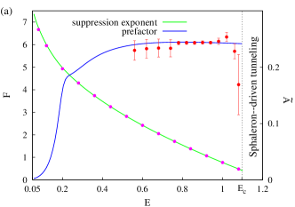
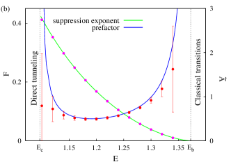
Figure 1: Comparison between the semiclassical (lines) and exact (points) results for the suppression exponent and prefactor in the cases of (a) direct and (b) sphaleron–driven tunneling. The comparison is performed in the model (2) with $\omega=0.5$, $E_{y}=0.05$. The error bars represent the uncertainty of the fit (17).

We checked the method of $\epsilon$–regularization by applying it to the model (2) and comparing the semiclassical results with the exact suppression exponent and prefactor extracted from the numerical solution to the Schrödinger equation. The latter quantities were obtained by fitting the dependence of the exact tunneling probability on $\hbar$ with the formula

$$\hbar\log{\cal P}(\hbar)\approx-F+\frac{\gamma}{2}\hbar\log\hbar+\hbar\log\tilde{A}\;,$$ (17)

where $\tilde{A}$ is independent of $\hbar$. For completeness, we also performed the comparison in the regime of direct tunneling. We set $\gamma=1$ for the direct tunneling and $\gamma=2$ in the sphaleron–driven case. Figure 1 shows the dependences $F(E)$ and $\tilde{A}(E)$ at fixed $E_{y}=0.05$. The semiclassical and exact quantum–mechanical calculations are in good agreement.

Note that the quality of the fit (17) becomes worse as one approaches the transition point $E_{c}$ between the two tunneling regimes. This is a manifestation of the breakdown of the semiclassical approximation in the vicinity of this point. It is caused by the change in the dependence of the prefactor on $\hbar$. Indeed, $\tilde{A}(E)$ diverges as $E\to E_{c}+0$, see Fig. 1b, which contradicts the continuity of the exact tunneling probability. However, the size of the vicinity where the semiclassical approximation breaks down vanishes in the limit $\hbar\to 0$.

Acknowledgements. We thank to F.L. Bezrukov, D.S. Gorbunov and V.A. Rubakov for discussions. This work was supported in part by the RFBR grant 05-02-17363, the Grants of the Russian Science Support Foundation (D.L. and S.S.), the Fellowship of the “Dynasty” Foundation (A.P.), and the EU 6th Framework Marie Curie Research and Training network ”UniverseNet” (MRTN-CT-2006-035863). The numerical calculations were performed on the Computational cluster of the Theoretical division of INR RAS.

References

- (1) O. Bohigas, S. Tomsovic and D. Ullmo, Phys. Rep. 223, 43 (1993); S. Takada, P.N. Walker and M. Wilkinson, Phys. Rev. A 52, 3546 (1995); A. Shudo, K.S. Ikeda, Phys. Rev. Lett. 74, 682 (1995); T. Van Voorhis, E.J. Heller, Phys. Rev. A 66, 050501(R) (2002); A.D. Ribeiro, M.A.M. de Aguiar, M. Baranger, Phys. Rev. E 69, 066204 (2004); S.C. Creagh, Nonlinearity 18, 2089 (2005); Phys. Rev. Lett. 98, 153901 (2007).
- (2) C. Dembowski et al, Phys. Rev. Lett. 84, 867 (2000).
- (3) W.K. Hensinger et al, Nature (London) 412, 52 (2001).
- (4) D.A. Steck, W.H. Oskay and M.G. Raizen, Science 293, 274 (2001).
- (5) W.H. Miller, Adv. Chem. Phys. 25, 69 (1974).
- (6) Tunneling in complex systems, edited by S. Tomsovic (World Scientific, Singapore, 1998).
- (7) F. Bezrukov and D. Levkov, arXiv:quant-ph/0301022; J. Exp. Theor. Phys. 98, 820 (2004) [Zh. Eksp. Teor. Fiz. 125, 938 (2004)].
- (8) K. Takahashi and K.S. Ikeda, J. Phys. A 36, 7953 (2003); Europhys. Lett. 71, 193 (2005).
- (9) F. Bezrukov, D. Levkov, C. Rebbi, V.A. Rubakov and P. Tinyakov, Phys. Rev. D 68, 036005 (2003); D.G. Levkov and S.M. Sibiryakov, Phys. Rev. D 71, 025001 (2005).
- (10) D.G. Levkov, A.G. Panin and S.M. Sibiryakov, arXiv:nlin.cd/0701063; arXiv:0704.0409 [quant-ph].
- (11) K. Takahashi and K.S. Ikeda, Phys. Rev. Lett. 97, 240403 (2006).
- (12) Unstable semiclassical solutions in a different context were studied in P.B. Wilkinson et al., Nature (London) 380, 608 (1996); S.C. Creagh and N.D. Whelan, Phys. Rev. Lett. 77, 4975 (1996); 82, 5237 (1998).
- (13) S. Levit and U. Smilansky, Ann. Phys. 103, 198 (1977).