AdS/CFT for Four-Point Amplitudes involving Gravitino Exchange

Abstract:

In this paper we compute the tree-level four-point scattering amplitude of two dilatini and two axion-dilaton fields in type IIB supergravity in $AdS_{5}\times S^{5}$. A special feature of this process is that there is an “exotic” channel in which there are no single-particle poles. Another novelty is that this process involves the exchange of a bulk gravitino. The amplitude is interpreted in terms of ${\cal N}=4$ supersymmetric Yang–Mills theory at large ’t Hooft coupling. Properties of the Operator Product Expansion are used to analyze the various contributions from single- and double-trace operators in the weak and strongly coupled regimes, and to determine the anomalous dimensions of semi-short operators. The analysis is particularly clear in the exotic channel, given the absence of BPS states.

1 Introduction

According to the AdS/CFT correspondence [1, 2, 3], the supergravity approximation to type II string theory in a $AdS_{5}\times S^{5}$ background corresponds to the strong ’tHooft coupling limit of $SU(N)$ $\mathcal{N}=4$ supersymmetric Yang–Mills theory, in the large $N$ limit.

The correspondence is easily checked for special protected processes that are independent of the ’t Hooft coupling, such as the two-point and three-point correlation functions of BPS states, which are completely determined by superconformal symmetry. The first non-trivial dependence on the coupling is observed in the correlation function of four BPS operators, which provides non-trivial information about the dynamics of the theory on the strongly coupled regime, via the correspondence (see [4] for references). Several examples have been worked out explicitly [5, 6, 7, 8, 9, 10, 11]. These have given rise to various exact and partial non-renormalization theorems for correlators in Yang-Mills theory (see [12] for reviews), and have shown that indeed there is a closed operator algebra in $\mathcal{N}=4$ SYM theory, and the amplitudes can be given an operator product expansion (OPE) interpretation [13, 14].

In [10] the correlation function of four superconformal primaries (CPO’s) in type IIB supergravity in $AdS_{5}\times S^{5}$ was evaluated in the tree approximation and used to determine the strongly coupled OPE of two operators in $\mathcal{N}=4$ SYM theory in the large $N$ limit. This expression was then compared with that obtained in free field theory, and the results were used to gain evidence for how the OPE expansion of two CPO’s changes as the coupling varies. More explicitly, the main idea in [10] was to consider the limit of the SYM correlator

$$\langle{\cal{O}}_{1}(\vec{x}_{1}){\cal{O}}_{2}(\vec{x}_{2}){\cal{O}}_{3}(\vec{x}_{3}){\cal{O}}_{4}(\vec{x}_{4})\rangle$$ (1)

in which $\vec{x}_{1}\rightarrow\vec{x}_{2}$ and $\vec{x}_{3}\rightarrow\vec{x}_{4}$ simultaneously. This amounts to doing a double OPE expansion of the form

$$\langle{\cal{O}}_{1}(\vec{x}_{1}){\cal{O}}_{2}(\vec{x}_{2}){\cal{O}}_{3}(\vec{x}_{3}){\cal{O}}_{4}(\vec{x}_{4})\rangle\sim\sum_{m,n}\frac{C_{12m}C_{34n}\langle{\cal{O}}_{m}(\vec{x}_{2}){\cal{O}}_{n}(\vec{x}_{4})\rangle}{|\vec{x}_{1}-\vec{x}_{2}|^{\Delta_{1}+\Delta_{2}-\Delta_{m}}|\vec{x}_{3}-\vec{x}_{4}|^{\Delta_{3}+\Delta_{4}-\Delta_{n}}}\cdots$$ (2)

where we have only shown the leading singular terms explicitly and $\Delta_{i}$ is the conformal dimension of ${\cal{O}}_{i}$. In this way, from the computation of the four-point function in the supergravity approximation, one can obtain the OPE of any two of the operators in strongly coupled Yang-Mills at large $N$. Comparison with the free field theory expression made it possible to deduce some interesting features concerning the coupling constant dependence of the anomalous dimensions of the intermediate single–trace and double–trace operators that contribute in the $(\vec{x}_{1}-\vec{x}_{2})$ channel.

It follows that the OPE at strong coupling is very different from the structure at weak coupling. On the free field theory there are huge degeneracies of states with finite conformal dimensions, but most of these are long (unprotected) states that develop anomalous dimensions of $O((g_{YM}^{2}N)^{1/4})$ at strong coupling and completely decouple from the OPE. These are known to correspond, on the gravity side of the correspondence, to excited string states that disappear upon taking the supergravity limit. There are also a number of states that pick up anomalous dimensions but do not diverge in the supergravity limit $g_{YM}^{2}N\to\infty$. Apart from the well-known short operators, states of this type include semi-short (double-trace) operators with dimensions that get corrections of order $1/N^{2}$.

Similar OPE interpretations have been obtained for the case of four superconformal scalar descendents (operators dual to the type II dilaton-axion with $\Delta=4$) in [13, 14], but up to now there has been no study of four-point correlation functions involving fermionic operators in the superconformal multiplet (although the exchange of a generic $1/2$-spin field exchange was considered in [15]). Such correlators will generically involve AdS diagrams with an exchange of a massless gravitino in the bulk, and this type of process has not been considered before, mainly because of the absence of a viable expression for the massless propagator [17].

Various techniques for computing four-point exchange diagrams were developed by Freedman and D’Hoker in a series of papers [18, 19]. Initially, evaluation of these diagrams involved the integration over one AdS vertex of the bulk-to-bulk propagator which was carried out by means of a tedious expansion and resumation procedure. Later on, the same group developed a new method [20] which circumvented the explicit evaluation of the integral, and did not required the knowledge of the relevant bulk-to-bulk propagator, making the evaluation a much simpler affair. The key point in this procedure is the fact that the propagator couples to conserved currents and satisfies an appropiate wave equation away from the source. In this paper, we will extend this procedure to the case of a massless gravitino exchange by studying the process

$$\langle{\mathcal{O}}_{\tau}(\vec{x}_{1})\Lambda_{i}(\vec{x}_{2}){\bar{\mathcal{O}}}_{\tau}(\vec{x}_{3})\bar{\Lambda}^{i}(\vec{x}_{4})\rangle$$ (3)

where ${\mathcal{O}}_{\tau}$ and $\Lambda_{i}$ are the operators transforming under $\mathbf{1}$ and $\mathbf{\bar{4}}$ of $SU(4)$, with conformal weights $\Delta=4$ and $\Delta=7/2$ respectively. These operators belong to the $1/2$-BPS current multiplet, and are related to $\mathcal{O}_{2}$, the superconformal primary, by supersymmetry transformations $\delta^{4}\mathcal{O}_{2}\sim\mathcal{O}_{\tau}$, $\delta^{3}\mathcal{O}_{2}\sim\Lambda$ (with $\delta$ denoting a $Q$-transformation).

Although this process is related by supersymmetry to the four-point function of CPO’s, it has several novel features. In the supergravity approximation it receives contributions from two exchange diagrams -a graviton exchange in the $(\vec{x}_{1}-\vec{x}_{3})$ channel and a gravitino exchange in the $(\vec{x}_{1}-\vec{x}_{4})$ channel-, together with a contact interaction. There is no single–particle exchange in the $(\vec{x}_{1}-\vec{x}_{2})$ channel, which follows from the $U(1)$ R-symmetry of supergravity . We will refer to the $(\vec{x}_{1}-\vec{x}_{2})$ channel as the “exotic” channel, in line with the older terminology for meson scattering. Computation of this process will also allow us to study the OPE of fermionic operators, and their behaviour under variation of the coupling. In particular, we will focus on the OPE ${\mathcal{O}}_{\tau}(\vec{x}_{1})\Lambda(\vec{x}_{2})$, which is known to contain a semi-short operator which is dual to a bound state in the gravity theory. This semi-short operator may be of relevance for understanding the truncation performed in [22].

This paper is organized as follows. In Section 2 we summarize our results. In Section 3 we derive the effective action of type IIB supergravity, compactified on $AdS_{5}\times S^{5}$, which is required for the computation and compute the corresponding supergravity four-point amplitude. We separately describe the contributions coming from the graviton and gravitino exchanges, and the contact graph, focusing on the generalization of the method [20] for the massless spin $3/2$ case. This result is in agreement with the one obtained in [23] using superconformal techniques . In Section 4 we will use free $\mathcal{N}=4$ SYM field theory to derive OPE’s of relevance to the correlation function (3) in various short-distance limits. This will be compared with the analogous limits of the supergravity result, which corresponds to the strongly coupled gauge theory. From this we will determine the fate of certain non-BPS states when the theory becomes strongly coupled. The discussion and conclusions are presented in Section 5. We also include two appendices that provide technical details concerning $D$-functions, that enter the expression for the amplitude.

2 Summary of the supergravity amplitude

The detailed evaluation of the three diagrams that contribute to the amplitude will be given in section 3. For clarity we will now summarize the results. The complete contribution to the four-point function in the supergravity approximation, is given by

$$\langle{\mathcal{O}}_{\tau}(\vec{x}_{1})\Lambda(\vec{x}_{2}){\bar{\mathcal{O}}}_{\tau}(\vec{x}_{3})\bar{\Lambda}(\vec{x}_{4})\rangle = \frac{\not{\vec{x}}_{24}}{|\vec{x}_{13}|^{8}|\vec{x}_{24}|^{8}}$$ (4)

$$+ \frac{1}{3N^{2}}\frac{1}{|\vec{x}_{13}|^{8}|\vec{x}_{24}|^{8}}\left[I_{graviton}+I_{gravitino}+I_{quartic}\right]$$

where the first term is the disconnected contribution, and the term of order $1/N^{2}$ gives the connected contribution. Here

$$I_{graviton} = \Big{[}(u+v)\left(6\bar{D}_{2525}+8\bar{D}_{3535}+5\bar{D}_{4545}\right)-2\bar{D}_{1414}-8\bar{D}_{2424}-8\bar{D}_{3434}$$

$$+ \left.11\bar{D}_{4444}-\frac{5}{2}\bar{D}_{5454}-\frac{3}{2}(\bar{D}_{3526}-\bar{D}_{2536})-\frac{5}{2}(\bar{D}_{4536}-\bar{D}_{3546})\right]\not{\vec{x}_{24}}$$

$$+ \left[3(\bar{D}_{2536}-\bar{D}_{3526})+5(\bar{D}_{3546}-\bar{D}_{4536})\right]\frac{\not{\vec{x}_{23}}\not{\tilde{x}_{31}}\not{\vec{x}_{14}}}{|\vec{x}_{13}|^{2}}$$

$$I_{gravitino} = \left[4\bar{D}_{2442}+6\bar{D}_{3443}-16\bar{D}_{4444}-6\bar{D}_{3452}-8\bar{D}_{4453}+10\bar{D}_{5454}\right]\not{\vec{x}_{24}}$$

$$+ \left[-6\bar{D}_{2552}-12\bar{D}_{3553}-10\bar{D}_{4554}+2\bar{D}_{2451}+6\bar{D}_{3452}+6\bar{D}_{4453}\right]\frac{\not{\vec{x}_{23}}\not{\tilde{x}_{31}}\not{\vec{x}_{14}}}{|\vec{x}_{13}|^{2}}$$

$$I_{quartic} = [15\bar{D}_{5445}-30\bar{D}_{4444}]\not{\vec{x}_{24}}-15\bar{D}_{5454}\frac{\not{\vec{x}_{23}}\not{\vec{x}_{31}}\not{\vec{x}_{14}}}{|\vec{x}_{13}|^{2}}$$ (5)

The $\bar{D}$-functions, $\bar{D}_{\Delta_{1}\Delta_{2}\Delta_{3}\Delta_{4}}(u,v)$, are standard four-point contact diagrams in AdS, involving the contact interaction of four scalars of conformal dimensions $\Delta_{i}$ which depend on the conformal ratios

$$u=\frac{|\vec{x}_{12}|^{2}|\vec{x}_{34}|^{2}}{|\vec{x}_{13}|^{2}|\vec{x}_{24}|^{2}}\quad v=\frac{|\vec{x}_{14}|^{2}|\vec{x}_{23}|^{2}}{|\vec{x}_{13}|^{2}|\vec{x}_{24}|^{2}}$$ (6)

In section 4 we will analyze this amplitude in various short distance limits, in order to determine properties of its intermediate states.

3 Supergravity Four-Point Function

The precise statement of the AdS/CFT correspondence that allows us to compute correlation functions of Yang-Mills operators from the supergravity AdS theory, was given by Witten in [3]. In a schematic form, one has

$$\mathrm{exp}\left\{-S_{IIB}[\phi]\right\}=\left\langle\mathrm{exp}\left(\int_{\partial(AdS)}\mathcal{O}\phi_{0}\right)\right\rangle_{YM}$$ (7)

where $\phi$ denotes the solution of the supergravity equations of motion, and the value of $\phi$ at the boundary of AdS, is identified with the source $\phi_{0}$ that couples to a conformal field $\mathcal{O}$.

We will focus on operators that belong to the well-known $1/2$ BPS current multiplet [24], which are dual to fields on the gravity supermultiplet of type IIB sugra on $AdS_{5}\times S^{5}$. Some four-point function of these operators have been computed before, namely, those involving the top operators of the multiplet, or chiral primaries [6], and the bottom operators of the multiplet, which transform as singlets of $SU(4)$ [19]. In the present case, we will explore the correlation function $\langle{\mathcal{O}}_{\tau}(\vec{x}_{1})\Lambda_{i}(\vec{x}_{2}){\bar{\mathcal{O}}}_{\tau}(\vec{x}_{3})\bar{\Lambda}^{i}(\vec{x}_{4})\rangle$, where ${\mathcal{O}}_{\tau}$ and $\Lambda_{i}$ are the operators transforming under $\mathbf{1}$ and $\mathbf{\bar{4}}$ of $SU(4)$, and conformal weights $\Delta=4$ and $\Delta=7/2$ respectively. Before proceeding with the calculation, let us first analyze the supergravity fields to which they are dual.

The operators ${\mathcal{O}}_{\tau}$ and ${\bar{\mathcal{O}}}_{\tau}$ enter the Yang-Mills action as

$$S=\frac{i}{4\tau_{2}}\int d^{4}x\Big{[}\tau{\mathcal{O}}_{\tau}-\bar{\tau}{\bar{\mathcal{O}}}_{\tau}\Big{]}$$ (8)

where $\tau=\frac{\theta_{YM}}{4\pi}+i\frac{4\pi}{g_{YM}^{2}}=\tau_{1}+i\tau_{2}$ is the complex coupling constant. Hence one could naively think ${\mathcal{O}}_{\tau}$ is sourced by $\tau/\tau_{2}$ in supergravity, where $\tau$ is the axion-dilaton complex scalar $\tau=C_{0}+ie^{\phi}$, but this is not true as it does not transform as a modular form under the the $SL(2,Z)$ symmetry. The source is in fact $i(\delta\tau)/{\sqrt{2}}\tau_{2}$ which is a modular form of weight $(-1,1)$. So at the linearized level, ${\mathcal{O}}_{\tau}$ is sourced by $i(\delta\tau)/{\sqrt{2}}\tau_{2}^{0}$ where $\tau_{2}^{0}$ stands for the background value of $\tau_{2}$. In this way, the relevant field for our computations is identified to be

$$P_{\mu}=\frac{i}{2}\frac{\partial_{\mu}\tau}{\tau_{2}}$$ (9)

The spin $1/2$ operators, $\Lambda_{i}$ and $\bar{\Lambda}^{i}$, are easier to identify, and from the quantum numbers, one can see they are sourced by the massless dilatino of the supergravity theory. Having identified the bulk fields, one can start by finding the relevant couplings from the IIB supergravity equations of motion [21, 25], and its Kaluza-Klein reduction to $d=5$ [26].

3.1 Results of the Reduction

We first write down the relevant terms in the $d=10$ type IIB supergravity action, and then obtain the $d=5$ action. In the absence of a simple action of this chiral supergravity that implements the self–duality of the five–form field strength at the level of the action, we consider the covariant equations of motion which give us the relevant terms in the action. We focus on the fermionic terms as the bosonic terms have been written down before [27], and use a hat to denote ten dimensional fields. Considering the linearized equations of motion for the dilatino $\hat{\Lambda}$ and the gravitino $\psi_{M}$ given by (see (4.6) and (4.12) of [21]).

$$\Gamma^{M}D_{M}\hat{\Lambda}-i\frac{\kappa_{10}g_{s}}{240}\Gamma^{M_{1}\ldots M_{5}}\hat{\Lambda}F_{M_{1}\ldots M_{5}}=0$$

$$\Gamma^{MNP}D_{N}\psi_{P}-\frac{1}{4\tau_{2}}(\partial_{N}\tau)\Gamma^{N}\Gamma^{M}\hat{\Lambda}^{*}+i\frac{\kappa_{10}g_{s}}{480}\Gamma^{MNP}\Gamma^{PQRST}\Gamma_{N}\psi_{P}F_{PQRST}=0$$ (10)

we get the action

$$S=\int d^{10}x{\sqrt{-g^{\prime}}} \Big{[} 2\hat{P}^{M}\hat{P}^{*}_{M}+\bar{\hat{\Lambda}}\Gamma^{M}D_{M}\hat{\Lambda}+{\bar{\psi}}_{M}\Gamma^{MNP}D_{N}\psi_{P}$$ (11)

$$- i\frac{\kappa_{10}g_{s}}{240}\bar{\hat{\Lambda}}\Gamma^{M_{1}\ldots M_{5}}\hat{\Lambda}F_{M_{1}\ldots M_{5}}+\frac{i}{2}\hat{P}_{N}{\bar{\psi}}_{M}\Gamma^{N}\Gamma^{M}\hat{\Lambda}^{*}$$

$$+ \frac{i}{2}\hat{P}^{*}_{N}\bar{\hat{\Lambda}}^{*}\Gamma^{M}\Gamma^{N}\psi_{M}+i\frac{\kappa_{10}g_{s}}{480}{\bar{\psi}}_{M}\Gamma^{MNP}\Gamma^{PQRST}\Gamma_{N}\psi_{P}F_{PQRST}\Big{]}.$$

We consider the fields in the $SL(2,R)/U(1)$ formulation, in which the axion-dilaton complex scalar $\hat{\tau}$ is contained in the $SL(2,R)$ singlet, $\hat{P}_{M}$, so in the $\varphi=0$ gauge [28] takes the form

$$\hat{P}_{M}=\frac{i}{2}\frac{\partial_{M}\hat{\tau}}{\hat{\tau_{2}}}$$ (12)

The covariant derivative $D_{M}$ appearing in the action contains not only the spin-connection, but also the $U(1)$ connection $Q_{M}$, so again in the $\varphi=0$ gauge, the term appearing in the derivative has the form $-q\frac{\partial_{M}\hat{\tau}}{2\hat{\tau}}$, where $q$ is the $U(1)$ charge.

One can then obtain the relevant couplings from the Kaluza-Klein reduction of (11) on $AdS_{5}\times S^{5}$. The quadratic terms have been computed in [27], and are given by

$$S_{\rm{quad}}=\frac{1}{2\kappa_{5}^{2}}\int_{AdS_{5}}d^{5}x{\sqrt{-g}} \left[R-\frac{|\partial_{\mu}\tau|^{2}}{2\tau_{2}^{2}}+\bar{\Lambda}_{i}\left(\Gamma^{\mu}D_{\mu}+\frac{3}{2}\right)\Lambda^{i}\right.$$ (13)

$$+ \left.{\bar{\psi}}_{\mu}^{i}\left(\Gamma^{\mu\nu\rho}D_{\nu}\psi_{\rho i}+\frac{3}{2}\Gamma^{\mu\nu}\psi_{\nu i}\right)\right]$$

which yields a dilatino and a gravitino of mass $-3/2$ . Note that both masses satisfy the relation

$$|m|=\Delta-2$$ (14)

since $\Delta=7/2$ for both dual operators in the gauge theory. We have also rescaled the fermion fields so that the full action has an overall factor of $1/2\kappa_{5}^{2}$.

The cubic terms can also be obtained from reduction of the ten-dimensional action. These are given by

$$S_{\rm{cubic}}=-\frac{1}{2\kappa_{5}^{2}}\int_{AdS_{5}}d^{5}x\sqrt{-g} \Big{[} \frac{1}{4\tau_{2}}(\partial_{\mu}\tau){\bar{\psi}}_{\nu}^{i}\Gamma^{\mu}\Gamma^{\nu}\Lambda^{*}_{i}-\frac{1}{4\tau_{2}}(\partial_{\nu}\bar{\tau})\bar{\Lambda}^{*i}\Gamma^{\mu}\Gamma^{\nu}\psi_{\mu i}$$ (15)

$$+ \frac{3}{8}i\bar{\Lambda}^{i}\Gamma^{\mu}\Lambda_{i}\frac{(\partial_{\mu}\tau)}{\tau_{2}}+\frac{3}{8}i\bar{\Lambda}^{i}\Gamma^{\mu}\Lambda_{i}\frac{(\partial_{\mu}\bar{\tau})}{\tau_{2}}\Big{]}$$

Here the terms in the second line are obtained from the $Q_{M}$ term in the ten-dimensional covariant derivative, when acting on the dilatino. The free theory fermionic actions in (13) need to be supplemented with certain boundary terms, as they vanish on-shell. These terms are defined on closed four dimensional submanifolds in $AdS_{5}$ in the limit when the submanifold approaches the boundary. The role of these boundary terms for spin 1/2 fermions has been studied in [29, 30, 31, 32], while for Rarita–Schwinger fields it has been analyzed in [33, 34, 35]. Although these terms will not affect our calculation in any way, they are included for completeness. These are

$$S_{\rm{bound}}=\frac{1}{2\kappa_{5}^{2}}\int_{\partial AdS_{5}}d^{4}\zeta\sqrt{-\bar{g}}\frac{1}{2}\left(\bar{\Lambda}_{i}\Lambda^{i}-{\bar{\psi}}^{i}_{m^{\prime}}{\bar{g}}^{m^{\prime}n^{\prime}}\psi_{in^{\prime}}\right)$$ (16)

where ${\bar{g}}_{m^{\prime}n^{\prime}}$ is the induced metric on the boundary.

We are now ready to compute the four-point function. As usual, we will work with the Euclidean version of $AdS_{5}$, so that the action is given by

$$S = \frac{1}{2\kappa_{5}^{2}}\int_{EAdS_{5}}d^{5}x{\sqrt{g}}\Big{[}-R+\frac{|\partial_{\mu}\tau|^{2}}{2\tau_{2}^{2}}+\bar{\Lambda}_{i}\left(\Gamma^{\mu}D_{\mu}+\frac{3}{2}\right)\Lambda^{i}$$ (17)

$$+ {\bar{\psi}}_{\mu}^{i}\left(\Gamma^{\mu\nu\rho}D_{\nu}\psi_{\rho i}+\frac{3}{2}\Gamma^{\mu\nu}\psi_{\nu i}\right)-\frac{1}{4\tau_{2}}\Big{(}(\partial_{\mu}\tau){\bar{\psi}}_{\nu}^{i}\Gamma^{\mu}\Gamma^{\nu}\Lambda^{*}_{i}-(\partial_{\nu}\bar{\tau})\bar{\Lambda}^{*i}\Gamma^{\mu}\Gamma^{\nu}\psi_{\mu i}\Big{)}\Big{.}$$

$$- \Big{.}\frac{3i}{8\tau_{2}}\left(\bar{\Lambda}_{i}\Gamma^{\mu}(\partial_{\mu}\tau)\Lambda^{i}+\bar{\Lambda}_{i}\Gamma^{\mu}(\partial_{\mu}\bar{\tau})\Lambda^{i}\right)\Big{]}$$

$$- \frac{1}{2}\int_{\partial EAdS_{5}}d^{4}\zeta\sqrt{\bar{g}}\left(\bar{\Lambda}_{i}\Lambda^{i}-{\bar{\psi}}^{i}_{m^{\prime}}{\bar{g}}^{m^{\prime}n^{\prime}}\psi_{in^{\prime}}\right).$$

The five dimensional axion and the dilaton are obtained in the obvious way from those in ten dimensions, while the graviton is obtained from the ten dimensional one using the relation $h_{\mu\nu}=h^{\prime}_{\mu\nu}+\frac{1}{3}(g_{0})_{\mu\nu}h^{\prime\alpha}_{\alpha}$, where $g_{0}$ is the $AdS_{5}$ metric and $h^{\prime\alpha}_{\alpha}$ is the trace of the graviton on $S^{5}$. Here

$$\frac{1}{2\kappa_{5}^{2}}=\frac{{\rm Vol}(S^{5})}{2g_{s}^{2}\kappa_{10}^{2}}=\frac{\pi^{3}R^{5}}{g_{s}^{2}(2\pi)^{7}\alpha^{\prime 4}}=\frac{N^{2}}{8\pi^{2}R^{3}}$$ (18)

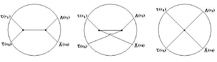
Figure 1: Witten diagrams contribuing to the process.

We can now see directly that the correlator will have one graviton exchange and one gravitino exchange in the bulk from the $t$ and $u$ channels respectively. There is also a contact diagram, coming from the quartic coupling that is contined in the $-\frac{3}{4}\bar{\hat{\Lambda}}_{i}\Gamma^{M}Q_{M}\hat{\Lambda}^{i}$ term in the Dirac action for $\hat{\Lambda}^{i}$. Figure 1 depicts the relevant diagrams contributing to the process. One should notice that this is all in agreement with the $U(1)$ symmetry of supergravity. The computation of these diagrams will be carried out in the following sections.

3.2 Graviton Exchange

As in most previous work, we work on Euclidean $AdS_{5}$ defined as the upper half space in $z^{\mu}\in\mathbf{R}^{5}$, with $z^{0}>0$, with the metric given by

$$ds^{2}=\sum_{\mu,\nu=0}^{d}g_{\mu\nu}dz^{\mu}dz^{\nu}=\frac{1}{z_{0}^{2}}(dz_{0}^{2}+\sum^{d}_{i=1}dz_{i}^{2})$$ (19)

The coordinates $z_{\mu}$ will be raised and lowered with the flat space metric unless otherwise mentioned. We shall choose the vielbein to be given by

$$e_{\mu}^{a}=\frac{1}{z_{0}}\delta_{\mu}^{a}$$ (20)

so that the spin and Levi-Civita connections are given by

$$w_{\mu}^{ab} = \frac{1}{z_{0}}(\delta^{a}_{0}\delta^{b}_{\mu}-\delta^{b}_{0}\delta^{a}_{\mu})$$

$$\Gamma^{\rho}_{\mu\nu} = \frac{1}{z_{0}}(\delta^{\rho}_{0}\delta_{\mu\nu}-\delta_{\mu 0}\delta^{\rho}_{\nu}-\delta_{\nu 0}\delta^{\rho}_{\mu})$$ (21)

where $a,b$ are tangent indices. The Dirac matrices in curved space will be related to those in the tangent space by $\Gamma^{\mu}=e^{\mu}_{a}\gamma^{a}$, so that $\{\gamma^{a},\gamma^{b}\}=2\delta^{ab}$. We now proceed to work out the amplitudes explicitly.

The supergravity calculation that we wish to address in this section, is the process involving an exchange of a massless graviton between two scalars and two spin $1/2$ fermions. In the setting of type IIB compactified on $AdS_{5}\times S^{5}$, one can identify the scalar as the axion-dilaton field and the fermion with the dilatino.

Now any supergravity operator $\hat{\cal{O}}(z)$ in the bulk can be expressed in terms of its boundary value $J_{{\cal{O}}}(\vec{x})$ which acts as the source for the composite operator ${\cal{O}}(\vec{x})$ in YM, as was indicated in [3]. The explicit relation is given by

$$\hat{\cal{O}}(z)=\int d^{d}\vec{x}K_{\Delta}(z,\vec{x})J_{{\cal{O}}}(\vec{x}),$$ (22)

where $K_{\Delta}(z,\vec{x})$ is the expression for the bulk–to–boundary propagator. For calculating the amplitude, the various expressions that are relevant are

$$i\frac{\delta\tau}{\sqrt{2}\tau_{2}}(z) = \int d^{4}\vec{x}~{}K_{4}(z,\vec{x})J_{\mathcal{O}_{\tau}}(\vec{x})$$

$$\Lambda_{i}(z) = \int d^{4}\vec{x}~{}K_{7/2}(z,\vec{x})\frac{(1+\gamma_{0})}{2}J_{i\Lambda}(\vec{x})$$

$$\bar{\Lambda}^{i}(z) = \int d^{4}\vec{x}~{}{\bar{J}}^{i}_{\Lambda}(\vec{x})\frac{(1-\gamma_{0})}{2}K_{7/2}(z,\vec{x})$$ (23)

Here $K_{4}(z,\vec{x})$ is the normalized bulk-to-boundary scalar propagator, which is given in general by

$$K_{\Delta}(z,\vec{x})=C_{\Delta}{\widetilde{K}}_{\Delta}(z,\vec{x})=\frac{\Gamma(\Delta)}{\pi^{d/2}\Gamma(\Delta-\frac{d}{2})}\frac{z_{0}^{\Delta}}{(z-\vec{x})^{2\Delta}},$$ (24)

and $K_{7/2}(z,\vec{x})$ is the spin 1/2 fermion propagator

$$K_{7/2}(z,\vec{x})=K_{4}(z,\vec{x})U(z-\vec{x})=K_{4}(z,\vec{x})\frac{(\not{z}-\not{\vec{x}})}{\sqrt{z}_{0}}$$ (25)

The starting point is the effective action (17). One needs to represent the solution to the equations of motion as $\phi=\phi^{0}+\delta\phi$ for a generic field, where $\phi^{0}$ is the solution of the linearized equation of motion with fixed boundary conditions, and $\delta\phi$ represents the physical field on the bulk. In order to proceed, it is useful to introduce the following conserved currents

$$T^{\mu\nu}=\frac{1}{2\tau_{2}^{2}}\left(D^{(\mu}\tau D^{\nu)}\bar{\tau}-\frac{1}{2}g^{\mu\nu}D^{\rho}\tau D_{\rho}\bar{\tau}\right)\qquad\tilde{T}^{\mu\nu}=\bar{\Lambda}\Gamma^{(\mu}\overleftrightarrow{D}^{\nu)}\bar{\Lambda}$$ (26)

One can write the graviton in terms of its Green function as

$$\delta g_{\mu\nu}(w)=\int[dz]G_{\mu\nu\mu^{\prime}\nu^{\prime}}(w,z)T^{\mu\nu}(z)$$ (27)

so using this expression, we find the on-shell value of the action that is relevant for this diagram

$$I_{graviton}=\frac{1}{4}\int[dz][dw]\tilde{T}^{\mu\nu}(w)G_{\mu\nu\mu^{\prime}\nu^{\prime}}(w,z)T^{\mu^{\prime}\nu^{\prime}}(z)$$ (28)

The next step is to express the fields in terms of their boundary values (Eq. (23)). In this way the contribution to the amplitude is given by

$$I_{graviton}=\frac{1}{4}\int[dw]\tilde{T}^{\mu\nu}(w,\vec{x}_{2},\vec{x}_{4})A_{\mu\nu}(w,\vec{x}_{1},\vec{x}_{3})$$ (29)

$$A_{\mu\nu}(w,\vec{x}_{1},\vec{x}_{3})=\int[dz]G_{\mu\nu\mu^{\prime}\nu^{\prime}}(w,z)T^{\mu^{\prime}\nu^{\prime}}(w,\vec{x}_{1},\vec{x}_{3})$$ (30)

where the vertex factors, are given by

$$T^{\mu\nu}(z,\vec{x}_{1},\vec{x}_{3}) = D^{\mu}K_{4}(w,\vec{x}_{1})D^{\nu}K_{4}(w,\vec{x}_{3})-\frac{1}{2}g^{\mu\nu}\partial_{\rho}K_{4}(w,\vec{x}_{1})D^{\rho}K_{4}(z,\vec{x}_{3})$$

$$\tilde{T}^{\mu\nu}(w,\vec{x}_{2},\vec{x}_{4}) = \frac{1}{2}\mathcal{P}_{+}K_{7/2}(w,\vec{x}_{2})(\Gamma^{\mu}\overleftrightarrow{D}^{\nu}+\Gamma^{\nu}\overleftrightarrow{D}^{\mu})K_{7/2}(w,\vec{x}_{4})\mathcal{P}_{-}$$ (31)

We will use the methods developed in [20] to compute this diagram, which take advantage of the fact that the vertices are covariantly conserved. By inversion, one can see that the $z$-integral can be expressed as

$$A_{\mu\nu}(w,\vec{x}_{1},\vec{x}_{3})=C_{4}^{2}|\vec{x}_{31}|^{-8}\frac{J_{\mu\lambda}(w)}{w^{2}}\frac{J_{\nu\rho}(w)}{w^{2}}I_{\lambda\rho}(w^{\prime}-\vec{x}_{31}^{\prime})$$ (32)

where $J_{\mu\nu}(w)=\delta_{\mu\nu}-2\frac{w_{\mu}w_{\nu}}{w^{2}}$ is the conformal jacobian and the primes denote inverted coordinates, $z_{\mu}^{\prime}=\frac{z_{\mu}}{z^{2}}$. The key idea for performing this integral, is to make an ansatz for $I_{\mu\nu}(w)$ that respects conformal invariance, and use the Green’s function for the graviton propagator. This was carried out in [20], and we reproduce the result here

$$I_{\mu\nu}(w)=-\frac{2}{3}(t+t^{2}+t^{3})\left(\frac{\delta_{0\mu}\delta_{0\nu}}{w_{0}^{2}}-\frac{1}{3}g_{\mu\nu}\right)$$ (33)

where $t=(w_{0}/w)^{2}$. Substituting this expression back into (29), and inverting the other vertex, $\tilde{T}^{\mu\nu}(w,\vec{x}_{21},\vec{x}_{41})$, we see that there are two contributions to the amplitude, one proportional to $\tilde{T}_{00}$ and one proportional to ${\tilde{T}^{\mu}}_{\mu}$. The first contribution reads

$$I^{(1)}_{graviton}=-\frac{1}{6}\frac{C_{4}^{2}}{|\vec{x}_{21}||^{6}\vec{x}_{31}|^{8}|\vec{x}_{41}|^{6}} \int[dw]w_{0}(t+t^{2}+t^{3})\left\{\mathcal{P}_{+}K_{4}(w,\vec{x}_{21}^{\prime})\not{\vec{x}_{21}^{\prime}}U(w-\vec{x}_{21}^{\prime})\right.$$ (34)

$$\times \left.\left(\gamma_{0}\overleftrightarrow{\partial_{0}}+\overleftrightarrow{\partial_{0}}\gamma_{0}\right)U(w-\vec{x}_{41}^{\prime})\not{\vec{x}_{41}^{\prime}}K_{4}(w,\vec{x}_{41}^{\prime})\mathcal{P}_{-}\right\}$$

We can simplify this expression by using the following identities

$$\partial_{0}{U(w-\vec{x}^{\prime})K_{4}(w,\vec{x}^{\prime})} = \frac{7}{2w_{0}}U(w-\vec{x}^{\prime})K_{4}(w,\vec{x}^{\prime})-4U(w-\vec{x}^{\prime})K_{5}(w,\vec{x}^{\prime})+\frac{\gamma_{0}}{\sqrt{w_{0}}}K_{4}(w,\vec{x}^{\prime})$$

$$w_{0}\partial_{0}\tilde{K}_{4}(w,\vec{x}^{\prime}) = 4\tilde{K}_{4}(w,\vec{x}^{\prime})-8w_{0}\tilde{K}_{5}(w,\vec{x}^{\prime})$$ (35)

Hence we get

$$I^{(1)}_{graviton} = -\frac{1}{6}\frac{C_{4}^{4}}{|\vec{x}_{21}|^{6}\vec{x}_{31}|^{8}|\vec{x}_{41}|^{6}}\not{\vec{x}_{21}^{\prime}}\int[dw](t+t^{2}+t^{3})\left\{-\tilde{K}_{4}(w,\vec{x}_{21}^{\prime})\tilde{K}_{4}(w,\vec{x}_{41}^{\prime})\not{\vec{x}_{24}^{\prime}}\right.$$ (36)

$$+ \left[\tilde{K}_{4}(w,\vec{x}_{21}^{\prime})w_{0}\partial_{0}\tilde{K}_{4}(w,\vec{x}_{41}^{\prime})-\vec{x}_{21}^{\prime}\leftrightarrow\vec{x}_{41}^{\prime}\right]\times$$

$$\left.\left[(\not{\vec{w}}-\not{\vec{x}_{21}^{\prime}})+(\not{\vec{w}}-\not{\vec{x}_{41}^{\prime}})\right]\right\}\not{\vec{x}_{41}^{\prime}}\mathcal{P}_{-}$$

The second contribution reads

$$I^{(2)}_{graviton}=\frac{1}{18}\frac{C_{4}^{2}}{|\vec{x}_{21}|^{6}|\vec{x}_{31}|^{8}|\vec{x}_{41}|^{6}} \int[dw]w_{0}(t+t^{2}+t^{3})\left\{\mathcal{P}_{+}K_{4}(w,\vec{x}_{21}^{\prime})\not{\vec{x}_{21}^{\prime}}U(w-\vec{x}_{21}^{\prime})\right.$$ (37)

$$\times \left.\Gamma^{\mu}\overleftrightarrow{D}_{\mu}U(w-\vec{x}_{41}^{\prime})\not{\vec{x}_{41}^{\prime}}K_{4}(w,\vec{x}_{41}^{\prime})\mathcal{P}_{-}\right\}$$

which can be simplified using

$$\Gamma^{\mu}D_{\mu}(K_{4}(w,\vec{x}^{\prime})U(w-\vec{x}^{\prime}))=-\frac{3}{2}K_{4}(w,\vec{x}^{\prime})U(w-\vec{x}^{\prime})$$ (38)

resulting in

$$I^{(2)}_{graviton}=\frac{1}{6}\frac{C_{4}^{4}}{|\vec{x}_{21}|^{6}|\vec{x}_{31}|^{8}|\vec{x}_{41}|^{6}}\not{\vec{x}_{21}^{\prime}}\int[dw](t+t^{2}+t^{3})\tilde{K}_{4}(w,\vec{x}_{21}^{\prime})\tilde{K}_{4}(w,\vec{x}_{41}^{\prime})\not{\vec{x}_{24}^{\prime}}\not{\vec{x}_{41}^{\prime}}\mathcal{P}_{-}$$ (39)

By shifting $\vec{w}$ by $\vec{x}_{31}^{\prime}$, all integrals involved in (36) and (39) can be expressed in terms of $W$-functions [19], which are defined as

$${W_{k}}^{\Delta^{\prime}}(a,b)\equiv\int[dw]\frac{w^{2\Delta^{\prime}+2a+2k}_{0}}{w^{2k}}\frac{1}{(w-x)^{2\Delta^{\prime}}}\frac{1}{(w-y)^{2\Delta^{\prime}+2b}}$$ (40)

and in this case, $x\equiv\vec{x}_{23}^{\prime}$ and $y=\vec{x}_{43}^{\prime}$. These are essentially four-point contact diagrams in the inverted frame. In order to express the amplitude by means of $W$-functions, notice that one can replace $(\not{\vec{w}}-\not{\vec{x}^{\prime}})K_{\Delta}(w,\vec{x}^{\prime})$ by derivatives on $\vec{x}^{\prime}$, using the relation

$$\frac{(\not{\vec{w}}-\not{\vec{x}^{\prime}})}{w_{0}}\tilde{K}_{\Delta+1}(w,\vec{x}^{\prime})=\frac{1}{2\Delta}\tilde{K}_{\Delta}(w,\vec{x}^{\prime})$$ (41)

and then use the identity

$$\partial_{x_{i}}{W_{k}}^{\Delta^{\prime}}(a,b) = -2x_{i}\frac{k\Delta^{\prime}}{(k+\Delta^{\prime}+a-2)}{W_{k+1}}^{\Delta^{\prime}+1}(a-1,b-1)$$ (42)

$$- 2(x-y)_{i}\frac{\Delta^{\prime}(\Delta^{\prime}+b)}{(k+\Delta^{\prime}+a-2)}{W_{k}}^{\Delta^{\prime}+1}(a,b)$$

There are essentially four types of $W$-functions entering the graviton exchange. These are $W^{4}_{k}(0,0)$, $W^{4}_{k}(1,0)$, $W_{k}^{3}(2,2)$ and $\tilde{W}_{k}^{3}(2,2)$, with the tilde indicating $x\leftrightarrow y$. Performing the derivatives and inverting the coordinates, so that

$$\not{\vec{x}^{\prime}}_{21}\not{\vec{x}^{\prime}}_{43}\not{\vec{x}^{\prime}}_{41} = \frac{\not{\vec{x}}_{24}}{|\vec{x}_{21}|^{2}|\vec{x}_{41}|^{2}}+\frac{\not{\vec{x}}_{23}\not{\vec{x}}_{31}\not{\vec{x}}_{14}}{|\vec{x}_{21}|^{2}|\vec{x}_{31}|^{2}|\vec{x}_{41}|^{2}}$$

$$\not{\vec{x}^{\prime}}_{21}\not{\vec{x}^{\prime}}_{24}\not{\vec{x}^{\prime}}_{41} = -\frac{\not{\vec{x}}_{24}}{|\vec{x}_{21}|^{2}|\vec{x}_{41}|^{2}}\qquad\not{\vec{x}^{\prime}}_{21}\not{\vec{x}^{\prime}}_{23}\not{\vec{x}^{\prime}}_{41}=\frac{\not{\vec{x}}_{23}\not{\vec{x}}_{31}\not{\vec{x}}_{14}}{|\vec{x}_{21}|^{2}|\vec{x}_{31}|^{2}|\vec{x}_{41}|^{2}}$$ (43)

and writing $\not{\tilde{x}}\equiv x_{i}\gamma^{i}\mathcal{P}_{+}=x_{i}(\bar{\sigma}^{i})^{\dot{\alpha}\alpha}$ one can express the amplitude as

$$I_{graviton} = -\frac{1}{6}\frac{C_{4}^{4}}{|\vec{x}_{21}|^{8}|\vec{x}_{31}|^{8}|\vec{x}_{41}|^{8}}\sum_{k=1}^{3}\left\{\not{\vec{x}}_{24}\left[2W_{k}^{4}(0,0)+\frac{64}{(k+3)}W_{k}^{5}(1,0)\right.\right.$$ (44)

$$- \left.\frac{40}{(k+3)}(\tilde{W}^{4}_{k}(2,2)+W_{k}^{4}(2,2))+\frac{8k}{(k+3)}(W_{k+1}^{4}(1,1)-\tilde{W}_{k+1}^{4}(1,1))\right]$$

$$+ \left.\frac{\not{\vec{x}}_{23}\not{\tilde{x}}_{31}\not{\vec{x}}_{14}}{|\vec{x}_{31}|^{2}}\left[\frac{16k}{(k+3)}(W_{k+1}^{4}(1,1)-\tilde{W}_{k+1}^{4}(1,1))\right]\right\}$$

It is possible to translate between the $W$-functions and the more familiar $D$-functions, $D_{\Delta_{1}\Delta_{2}\Delta_{3}\Delta_{4}}$ [19], which are identified with quartic scalar interactions, and are related to the $W$-functions by inversion of coordinates. The explicit relation in this case, is given by

$${W_{k}}^{\Delta^{\prime}}(a,b)=|\vec{x}_{21}|^{2\Delta^{\prime}}|\vec{x}_{31}|^{2k}|\vec{x}_{41}|^{2(\Delta^{\prime}+b)}D_{2a-b+k,\Delta^{\prime},k,\Delta^{\prime}+b}$$ (45)

One can further, rewrite these in terms of conformal ratios, $u$ and $v$, by introducing $\bar{D}$-functions [8], whose properties are listed in appendix A. Using these, the expression for the graviton exchange contribution to the supergravity amplitude is given by

$$I_{graviton} = -\frac{\pi^{2}}{6}\frac{C_{4}^{4}}{|\vec{x}_{13}|^{8}|\vec{x}_{24}|^{8}}\left\{\left[\frac{1}{18}\bar{D}_{1414}+\frac{1}{6}\bar{D}_{2424}+\frac{1}{6}\bar{D}_{3434}+\frac{1}{12}\bar{D}_{3425}-\frac{1}{12}\bar{D}_{4253}+\frac{1}{9}\bar{D}_{4435}\right.\right.$$

$$- \left.\left.\frac{1}{9}\bar{D}_{4354}+\frac{5}{72}\bar{D}_{5445}-\frac{5}{72}\bar{D}_{4455}-\frac{1}{12}\bar{D}_{3416}-\frac{1}{12}\bar{D}_{4163}-\frac{1}{9}\bar{D}_{4426}-\frac{1}{9}\bar{D}_{4264}\right.\right.$$

$$- \left.\left.\frac{5}{72}\bar{D}_{5436}-\frac{5}{72}\bar{D}_{4365}+\frac{1}{6}\bar{D}_{2426}+\frac{2}{9}\bar{D}_{5254}+\frac{5}{36}\bar{D}_{5355}\right]\not{\vec{x}_{24}}\right.$$

$$+ \left.\left[\frac{1}{6}\bar{D}_{3425}-\frac{1}{6}\bar{D}_{4253}+\frac{2}{9}\bar{D}_{4435}-\frac{2}{9}\bar{D}_{4354}+\frac{5}{36}\bar{D}_{5445}+\frac{5}{36}\bar{D}_{4455}\right]\frac{\not{\vec{x}_{23}}\not{\tilde{x}_{31}}\not{\vec{x}_{14}}}{|\vec{x}_{13}|^{2}}\right\}$$

which can be further simplified using the identities (134,135) (some of the manipulations are included in appendix B).

$$I_{graviton} = \frac{\pi^{2}}{6}\frac{C_{4}^{4}}{|\vec{x}_{13}|^{8}|\vec{x}_{24}|^{8}}\left\{\left[(u+v)\left(\frac{1}{6}\bar{D}_{2525}+\frac{2}{9}\bar{D}_{3535}+\frac{5}{36}\bar{D}_{4545}\right)\right.\right.$$

$$- \frac{1}{18}\bar{D}_{1414}-\frac{2}{9}\bar{D}_{2424}-\frac{2}{9}\bar{D}_{3434}+\frac{11}{36}\bar{D}_{4444}-\frac{5}{72}\bar{D}_{5454}$$

$$- \left.\frac{1}{24}(\bar{D}_{3526}-\bar{D}_{2536})-\frac{5}{72}(\bar{D}_{4536}-\bar{D}_{3546})\right]\not{\vec{x}_{24}}$$

$$+ \left.\left[\frac{1}{12}(\bar{D}_{2536}-\bar{D}_{3526})+\frac{5}{36}(\bar{D}_{3546}-\bar{D}_{4536})\right]\frac{\not{\vec{x}_{23}}\not{\tilde{x}_{31}}\not{\vec{x}_{14}}}{|\vec{x}_{13}|^{2}}\right\}$$

This last expression explicitly shows that the amplitude is symmetric under exchange of $\vec{x}_{1}$ and $\vec{x}_{3}$, as one should expect since

$$\frac{\not{\vec{x}}_{23}\not{\tilde{x}}_{31}\not{\vec{x}}_{14}}{|\vec{x}_{13}|^{2}}=-\frac{\not{\vec{x}}_{21}\not{\tilde{x}}_{13}\not{\vec{x}}_{34}}{|\vec{x}_{13}|^{2}}-\not{\vec{x}}_{24}$$ (48)

It also transforms consistently under inversion, and respects the structure of the spinor indices, given that

3.3 Gravitino Exchange

We will now turn to the calculation of the gravitino exchange contribution, which is the novel part of the calculation. We will first generalize the procedure for computing $z$-integrals, and then we will express the result in a way that is consistent with superconformal symmetry. We will suppress spinor indices throughout this section, for simplicity.

Compactification of type IIB supergravity raises an interaction term between the massless gravitino and a current of the form

$$\mathcal{J}^{i\mu}=\frac{1}{\tau_{2}}(\partial_{\nu}\tau)\Gamma^{\nu}\Gamma^{\mu}\Lambda^{i*}$$ (49)

which satisfies a conservation equation of the form [36, 37]

$$\Big{(}D_{\mu}-\frac{\Gamma_{\mu}}{2}\Big{)}\mathcal{J}^{i\mu}=0,$$ (50)

with $D_{\mu}$ containing the spin connection and the Levi-Civita connection.

One can proceed as before, by writing the solution to the equation of motion as $\psi_{\mu}=\psi_{\mu}^{0}+\delta\psi_{\mu}$. The perturbation can then be expressed as

$$\delta\psi_{\mu}(w)=\int[dz]\Theta_{\mu\nu^{\prime}}(w,z)\mathcal{J}^{\nu^{\prime}}(z)$$ (51)

where $\Theta_{\mu\nu^{\prime}}(w,z)$ is the bulk-to-boundary propagator for the massless gravitino in $AdS$. Now we evaluate the action on-shell, to obtain the integral describing the gravitino exchange. Here one needs to be careful in taking into account the factors of $1/2\sqrt{2}$ that precedes the current, that determine the overall normalization. We then arrive at the expression

$$I_{gravitino}=\frac{1}{4}\int[dw]\bar{\mathcal{J}}^{\mu}(w,\vec{x}_{2},\vec{x}_{3})\psi_{\mu}(w,\vec{x}_{1},\vec{x}_{4})$$

$$\psi_{\mu}(w,\vec{x}_{1},\vec{x}_{4})=\int[dz]\Theta_{\mu\nu^{\prime}}(w,z)\mathcal{J}^{\nu^{\prime}}(z,\vec{x}_{1},\vec{x}_{4})$$ (52)

In principle, one could try to evaluate this expression using the explicit form for the $\Theta_{\mu\nu^{\prime}}(w,z)$, the bulk–to–bulk propagator for the massless gravitino [17]. However, it is simpler to generalize the method used for the graviton, to evaluate the $z$-integral. Using translation and conformal inversion, one can show that $\psi_{\mu}$ can be reexpressed as

$$\psi_{\mu}(w,\vec{x}_{1},\vec{x}_{4})=-\frac{\not{w}}{|w|}\frac{J_{\lambda\mu}(w)}{w^{2}}I_{\lambda}(w^{\prime}-\vec{x}_{41}^{\prime})\frac{\not{\vec{x}^{\prime}}_{41}}{|\vec{x}_{41}|^{6}}$$ (53)

where $J_{\mu\nu}(w)$ is the inversion jacobian defined before and

$$I_{\lambda}(z)=\int[dz]\Theta_{\lambda\lambda^{\prime}}(w,z)\Gamma^{\kappa^{\prime}}\Gamma^{\lambda^{\prime}}\partial_{\kappa^{\prime}}(z_{0}^{4})\frac{\not{z}}{\sqrt{z_{0}}}\left(\frac{z_{0}^{4}}{z^{8}}\right)\mathcal{P}_{+}$$ (54)

Once again, we must write down an ansatz for $I_{\lambda}(w)$. Scale symmetry, $d$-dimensional Poincairé symmetry and gauge invariance suggests

$$I_{\mu}(w)=\frac{1}{\sqrt{z_{0}}}\Big{(}\delta_{\mu 0}f_{1}(t)+\gamma_{\mu}f_{2}(t)+\frac{(w.\Gamma)}{w^{2}}\delta_{\mu 0}f_{3}(t)+\gamma_{\mu}\frac{(w.\Gamma)}{w^{2}}f_{4}(t)\Big{)}P_{+}$$ (55)

where $t=w_{0}^{2}/w^{2}$. The next step is to use the Rarita-Schwinger Green’s function equation for $\Theta_{\lambda\lambda^{\prime}}(w,z)$ to find an equation for $I_{\lambda}(w)$, namely

$${W_{\mu}}^{\rho}I_{\rho}(w)=\left(\Gamma_{\mu}\Gamma^{\nu}\Gamma^{\rho}D_{\nu}-\Gamma^{\rho}D_{\nu}-\Gamma_{\mu}D^{\rho}+\Gamma^{\nu}D_{\nu}\delta_{\mu}^{\rho}+\frac{3}{2}\Gamma_{\mu}\Gamma^{\rho}-\frac{3}{2}\delta_{\mu}^{\rho}\right)I_{\rho}(w)=\mathcal{\tilde{J}}_{\mu}(w)$$ (56)

with

$$\mathcal{\tilde{J}}_{\mu}(w) = \int[dz]\delta(z-w)g_{\mu\rho^{\prime}}\Gamma^{\nu}\Gamma^{\rho^{\prime}}\partial_{\nu}(z_{0}^{4})\frac{\not{z}}{\sqrt{z_{0}}}\left(\frac{z_{0}}{z^{2}}\right)^{4}\mathcal{P}_{+}$$ (57)

$$= \frac{4t^{3}}{\sqrt{w_{0}}}\left\{2\delta_{\mu 0}\frac{(w\cdot\Gamma)}{w^{2}}-2\gamma_{\mu}t+\gamma_{\mu}\frac{(w\cdot\Gamma)}{w^{2}}\right\}\mathcal{P}_{+}$$

Needless to say that the application of the wave operator is quite tedious. We simply give the results of these calculations. The left hand side of (56) reads

$${W_{\mu}}^{\rho}\left[\frac{\delta_{\rho 0}}{\sqrt{w_{0}}}f_{1}(t)\right]\mathcal{P}_{+} = \frac{1}{\sqrt{w_{0}}}\left[2tf_{1}^{\prime}(t)\left(w_{0}\frac{w_{\mu}}{w^{2}}-\delta_{\mu 0}\frac{(w\cdot\Gamma)}{w^{2}}-\gamma_{\mu}\frac{(w\cdot\Gamma)}{w^{2}}\right)\right.$$

$$+ \left.(2t^{2}f_{1}^{\prime}(t)+3f_{1}(t))\gamma_{\mu}-3f_{1}(t)\delta_{\mu 0}\right]\mathcal{P}_{+}$$

$${W_{\mu}}^{\rho}\left[\frac{\gamma_{\rho}}{\sqrt{w_{0}}}f_{2}(t)\right]\mathcal{P}_{+} = \frac{1}{\sqrt{w_{0}}}\left[(6tf_{2}^{\prime}(t)+3f_{2}(t))\left(\gamma_{\mu}-\delta_{\mu 0}\right)\right.$$

$$+ \left.6tf_{2}^{\prime}(t)\left(w_{0}\frac{w_{\mu}}{w^{2}}-\gamma_{\mu}\right)\frac{(w\cdot\Gamma)}{w^{2}}\right]\mathcal{P}_{+}$$

$${W_{\mu}}^{\rho}\left[\frac{\delta_{\rho 0}}{\sqrt{w_{0}}}\frac{(w\cdot\Gamma)}{w^{2}}f_{3}(t)\right]\mathcal{P}_{+} = \frac{1}{\sqrt{w_{0}}}\left[(2t^{2}f_{3}^{\prime}(t)+2tf_{3}(t))\left(\gamma_{\mu}-\delta_{\mu 0}-\gamma_{\mu}\frac{(w\cdot\Gamma)}{w^{2}}+2w_{0}\frac{w_{\mu}}{w^{2}}\right)\right.$$

$$- \left.(2tf_{3}^{\prime}(t)+2f_{3}(t))w_{0}w_{\mu}\frac{(w\cdot\Gamma)}{w^{4}}\right]\mathcal{P}_{+}$$

$${W_{\mu}}^{\rho}\left[\frac{\gamma_{\rho}}{\sqrt{w_{0}}}\frac{(w\cdot\Gamma)}{w^{2}}f_{4}(t)\right]\mathcal{P}_{+} = \frac{1}{\sqrt{w_{0}}}\left[(6tf_{4}^{\prime}(t)+6f_{4}(t))\left(t\gamma_{\mu}-\delta_{\mu 0}\frac{(w\cdot\Gamma)}{w^{2}}+w_{0}w_{\mu}\frac{(w\cdot\Gamma)}{w^{4}}\right)\right.$$ (58)

$$- \left.(6tf_{4}^{\prime}(t)-6f_{4}(t))\gamma_{\mu}\frac{(w\cdot\Gamma)}{w^{2}}\right]\mathcal{P}_{+}$$

So substitution of the ansatz (55) gives a set of equations for the undetermined coefficients $f_{i}(t)$. The system, however, is overdetermined, as it has 6 equations and 4 unknowns:

$$-3f_{1}(t)-6tf_{2}^{\prime}(t)-3f_{2}(t)-2t^{2}f_{3}^{\prime}(t)-2tf_{3}(t) = 0$$

$$2t^{2}f_{1}^{\prime}(t)+3f_{1}(t)+6tf_{2}^{\prime}(t)+3f_{2}(t)+2t^{2}f_{3}^{\prime}(t)+2tf_{3}(t)+6t^{2}f_{4}^{\prime}(t)+6tf_{4}(t) = -8t^{4}$$

$$-2f_{1}^{\prime}(t)-6tf_{2}^{\prime}(t)-2t^{2}f_{3}^{\prime}(t)-2tf_{3}(t)-6tf_{4}^{\prime}(t)+6f_{4}(t) = 4t^{3}$$

$$2tf_{1}^{\prime}(t)+6tf_{2}^{\prime}(t)+4t^{2}f_{3}^{\prime}(t)+4tf_{3}(t) = 0$$

$$-2tf_{1}^{\prime}(t)-6tf_{4}^{\prime}(t)-6f_{4}(t) = 8t^{3}$$

$$-2tf_{3}^{\prime}(t)-2f_{3}(t)+6tf_{4}^{\prime}(t)+6f_{4}(t) = 0$$ (59)

One must then look for a consistent solution. In this case it is given by

$$f_{1}(t) = -\frac{1}{3}(2t+3t^{2}+4t^{3})\qquad f_{2}(t)=\frac{1}{9}(2t+t^{2})$$

$$f_{3}(t) = \frac{1}{3}(t+2t^{2})\hskip 65.44133ptf_{4}(t)=\frac{1}{9}(t+2t^{2})$$ (60)

The functions above are regular on $t=1$, as expected, and vanish when $t$ approaches zero. Using these results on (53), one may compute $I_{gravitino}$. Upon inversion of the current $\bar{\mathcal{J}}^{\mu}$, the amplitude takes the form

$$I_{gravitino}=\frac{1}{4}\frac{C_{4}^{4}\not{\vec{x}^{\prime}}_{21}}{|\vec{x}_{21}|^{6}|\vec{x}_{31}|^{8}|\vec{x}_{41}|^{6}}\int[dw]\mathcal{P}_{-}\tilde{K}_{7/2}(w,\vec{x}_{21}^{\prime})\Gamma^{\lambda}\Gamma^{\nu}\partial_{\nu}(\tilde{K}_{4}(w,\vec{x}_{31}^{\prime}))I_{\lambda}(w-\vec{x}_{41}^{\prime})\not{\vec{x}^{\prime}}_{41}$$ (61)

Substituting (55) with (60), the resulting expression can be split into two contributions. To see this, we can rewrite the quantity between the chiral projectors, as

$$\mathcal{P}_{-}\tilde{K}_{7/2}(w,\vec{x}_{21}^{\prime})\Gamma^{\mu}\Gamma^{\nu}\partial_{\nu}\tilde{K}_{4}(w,\vec{x}_{31}^{\prime})I_{\mu}(w-\vec{x}_{41}^{\prime})=\mathcal{P}_{-}\tilde{K}_{4}(w,\vec{x}_{21}^{\prime})(\not{w}-\not{\vec{x}}_{21}^{\prime})\Big{[}\left(f_{1}(t)\gamma_{0}\right.$$

$$\left.\left.-3f_{2}(t)\right)\Gamma^{\nu}\partial_{\nu}\tilde{K}_{4}(w,\vec{x}_{31}^{\prime})-6tf_{4}(t)\mathcal{P}_{-}\Gamma^{\nu}\partial_{\nu}\tilde{K}_{4}(w,\vec{x}_{31}^{\prime})(\not{w}-\not{\vec{x}}_{41}^{\prime})\right]$$ (62)

The first contribution involves $f_{1}(t)$ and $f_{2}(t)$, whereas the second contribution is proportional to $f_{4}(t)$. We can simplify further by using the identity

$$\Gamma^{\mu}D_{\mu}\tilde{K}_{4}(w,\vec{x}^{\prime})=4\gamma_{0}\tilde{K}_{4}(w,\vec{x}^{\prime})-8(\not{w}-\not{\vec{x}^{\prime}})\tilde{K}_{5}(w,\vec{x}^{\prime})$$ (63)

so doing some algebra and simplifying, one gets

$$I_{gravitino}^{(1)}=-\frac{1}{3}\frac{C_{4}^{4}\not{\vec{x}_{21}^{\prime}}}{|\vec{x}_{21}|^{6}|\vec{x}_{31}|^{8}|\vec{x}_{41}|^{6}}\int[dw]\tilde{K}_{4}(w,\vec{x}_{21}^{\prime})w_{0}\partial_{0}\tilde{K}_{4}(w,\vec{x}_{31}^{\prime})(t+t^{2}+t^{3})(\not{\vec{w}}-\not{\vec{x}_{21}^{\prime}})\not{\vec{x}_{41}^{\prime}}\mathcal{P}_{-}$$ (64)

$$I_{gravitino}^{(2)}=-\frac{1}{6}\frac{C_{4}^{4}\not{\vec{x}_{21}^{\prime}}}{|\vec{x}_{21}|^{6}|\vec{x}_{31}|^{8}|\vec{x}_{41}|^{6}}\int[dw]\tilde{K}_{4}(w,\vec{x}_{21}^{\prime})w_{0}\partial_{0}\tilde{K}_{4}(w,\vec{x}_{31}^{\prime})(t^{2}+2t^{3})(\not{\vec{w}}-\not{\vec{x}_{41}^{\prime}})\not{\vec{x}_{41}^{\prime}}\mathcal{P}_{-}$$ (65)

The resulting integrals have the same form as those that occurred in the graviton case. Hence, we can make use of the same tricks. First we turn all terms of the form $(\not{\vec{w}}-\not{\vec{x}^{\prime}})$ into derivatives using (41), and then group in terms of $W$-functions, which were defined in (40), but taking $x\equiv\vec{x}_{24}^{\prime}$ and $y\equiv\vec{x}_{34}^{\prime}$. Then $I_{gravitino}^{(1)}$ can be rewritten in terms of $W_{k}^{3}(1,1)$ and $W_{k}^{3}(2,2)$, for $k=1,2,3$, and $I_{gravitino}^{(2)}$ in terms of $W_{k}^{4}(1,0)$ and $W_{k}^{4}(2,1)$, for $k=1,2$. Finally, one simplifies by doing the derivatives using (42) and inverting the coordinates as before, so $I_{gravitino}$ is given by

$$I_{gravitino} = -\frac{1}{3}\frac{C_{4}^{4}}{|\vec{x}_{21}|^{8}|\vec{x}_{31}|^{8}|\vec{x}_{41}|^{8}}\left[\sum_{k=1}^{3}\left\{\not{\vec{x}}_{24}\left[\frac{4k}{(k+2)}W_{k+1}^{4}(0,0)-\frac{8k}{(k+3)}W_{k+1}^{4}(1,1)\right]\right.\right.$$ (66)

$$+ \left.\frac{\not{\vec{x}}_{23}\not{\tilde{x}}_{31}\not{\vec{x}}_{14}}{|\vec{x}_{31}|^{2}}\left[-\frac{16}{(k+2)}W_{k}^{4}(1,1)+\frac{40}{(k+3)}W_{k}^{4}(2,2)\right]\right\}+\sum_{k=1}^{2}\left\{\not{\vec{x}}_{24}\left[-\frac{8k}{(k+3)}\times\right.\right.$$

$$+ \left.\left.(\tilde{W}_{k+1}^{4}(1,1)+W_{k+1}^{4}(1,1))+\frac{2k}{(k+3)}(8W_{k+1}^{5}(1,0)+10W_{k+1}^{4}(2,2))\right]\right.$$

$$+ \left.\left.\frac{\not{\vec{x}}_{23}\not{\tilde{x}}_{31}\not{\vec{x}}_{14}}{|\vec{x}_{31}|^{2}}\left[-\frac{8k}{(k+3)}W_{k+1}^{4}(1,1)+\frac{20k}{(k+4)}W_{k+1}^{4}(2,2)\right]\right\}\right]$$

Again, it is possible to translate between $W$-functions and $D$-functions. In this case, the relation is

$$W_{k}^{\Delta^{\prime}}(a,b)=|\vec{x}_{21}|^{2\Delta^{\prime}}|\vec{x}_{31}|^{2(\Delta^{\prime}+b)}|\vec{x}_{41}|^{2k}D_{2a-b+k,\Delta^{\prime},\Delta^{\prime}+b,k}$$ (67)

From here it is straightforward to rewrite the gravitino exchange diagram in terms of conformal invariant rations, by introducing the $\bar{D}$-functions. The amplitude then reads

$$I_{gravitino} = -\frac{\pi^{2}}{3}\frac{C^{4}_{4}}{|\vec{x}_{13}|^{8}|\vec{x}_{24}|^{8}}\left\{\left[\frac{1}{9}\bar{D}_{2442}+\frac{1}{6}\bar{D}_{3443}+\frac{1}{9}\bar{D}_{4444}-\frac{1}{6}\bar{D}_{3452}-\frac{2}{9}\bar{D}_{4453}\right.\right.$$ (68)

$$- \frac{5}{72}\bar{D}_{5454}+\frac{1}{18}\bar{D}_{4462}+\frac{5}{72}\bar{D}_{5463}-\frac{1}{12}\bar{D}_{2453}-\frac{1}{9}\bar{D}_{3452}+\frac{1}{18}\bar{D}_{3463}$$

$$+ \left.\frac{5}{72}\bar{D}_{4464}\right]\not{\vec{x}_{24}}+\left[-\frac{1}{9}\bar{D}_{2451}-\frac{1}{4}\bar{D}_{3452}-\frac{2}{9}\bar{D}_{4453}+\frac{1}{12}\bar{D}_{3461}\right.$$

$$+ \left.\left.\frac{1}{6}\bar{D}_{4462}+\frac{5}{36}\bar{D}_{5463}\right]\frac{\not{\vec{x}_{23}}\not{\tilde{x}_{31}}\not{\vec{x}_{14}}}{|\vec{x}_{13}|^{2}}\right\}$$

This expression can be shortened by using the identities of appendix A, as described in appendix B. The final expression one is left with is then

$$I_{gravitino} = \frac{\pi^{2}}{3}\frac{C^{4}_{4}}{|\vec{x}_{13}|^{8}|\vec{x}_{24}|^{8}}\left\{\left[\frac{1}{18}\bar{D}_{2442}+\frac{1}{12}\bar{D}_{3443}-\frac{2}{9}\bar{D}_{4444}-\frac{1}{12}\bar{D}_{3452}-\frac{1}{9}\bar{D}_{4453}\right.\right.$$ (69)

$$+ \left.\frac{5}{36}\bar{D}_{5454}\right]\not{\vec{x}}_{24}+\left[\frac{1}{36}\bar{D}_{2451}+\frac{1}{12}\bar{D}_{3452}+\frac{1}{12}\bar{D}_{4453}-\frac{1}{12}\bar{D}_{2552}-\frac{1}{6}\bar{D}_{3553}\right.$$

$$- \left.\left.\frac{5}{36}\bar{D}_{4554}\right]\frac{\not{\vec{x}_{23}}\not{\tilde{x}_{31}}\not{\vec{x}_{14}}}{|\vec{x}_{13}|^{2}}\right\}$$

3.4 Quartic Diagram

The last diagram that one needs to compute is the quartic interaction. The necessary couplings are obtained from the cubic vertices involving two dilatinos and $P_{\mu}$, by considering variations of the dilaton factor $\tau_{2}^{-1}$. The relevant terms in the action become

$$I_{quartic}=\int[dz]\left[\frac{3}{8}\bar{\hat{\Lambda}}\Gamma^{\mu}\partial_{\mu}\left(\frac{i\delta\tau}{\sqrt{2}\tau_{2}}\right)\left(-\frac{i\delta\bar{\tau}}{\sqrt{2}\tau_{2}}\right)\hat{\Lambda}-\frac{3}{8}\bar{\hat{\Lambda}}\Gamma^{\mu}\partial_{\mu}\left(-\frac{i\delta\bar{\tau}}{\sqrt{2}\tau_{2}}\right)\left(\frac{i\delta\tau}{\sqrt{2}\tau_{2}}\right)\hat{\Lambda}\right]$$ (70)

We now proceed as before. One replaces the bulk fields in terms of their boundary values. There will be two contributions to the diagram, coming from interchange of the fields in $x_{1}$ and $x_{3}$. We compute explicitly one of the contributions, and obtain the second by interchange of $\vec{x}_{1}$ and $\vec{x}_{3}$, and some simple manipulations involving the $\bar{D}$-functions and $\Gamma$-matrices.

The integral arising from the action has the structure

$$\int[dw]\mathcal{P}_{+}U(w-\vec{x}_{2})K_{4}(w,\vec{x}_{2})\Gamma^{\mu}\partial_{\mu}K_{4}(w,\vec{x}_{3})K_{4}(w,\vec{x}_{1})K_{4}(w,\vec{x}_{4})U(w-\vec{x}_{4})\mathcal{P}_{-}$$ (71)

Using translation invariance we can set $\vec{x}_{4}\to 0$. Furthermore, one can invert the expression to make the integrand simpler

$$\frac{-\not{\vec{x}_{24}^{\prime}}C_{4}^{4}}{|\vec{x}_{24}^{\prime}|^{-6}|\vec{x}_{34}^{\prime}|^{-8}|\vec{x}_{14}^{\prime}|^{-8}}\int[dw]\mathcal{P}_{-}\tilde{K}_{4}(w,\vec{x}_{24}^{\prime})\tilde{K}_{4}(w,\vec{x}_{14}^{\prime})U(w-\vec{x}_{24}^{\prime})\Gamma^{\mu}\partial_{\mu}\tilde{K}_{4}(w,\vec{x}_{34}^{\prime})\frac{w_{0}^{4}}{\sqrt{w_{0}}}\mathcal{P}_{-}$$ (72)

The integrand can be simplified by working out the gamma-matrix algebra, by using similar manipulations as the ones performed in previous sections. It is then simple to rewrite this integral as a sum of a single gamma-matrix term, and a triple-gamma matrix term

$$\frac{\not{\vec{x}_{24}^{\prime}}C_{4}^{4}}{|\vec{x}_{24}^{\prime}|^{-6}|\vec{x}_{34}^{\prime}|^{-8}|\vec{x}_{14}^{\prime}|^{-8}}\int[dw]\tilde{K}_{4}(w,\vec{x}_{24}^{\prime})\tilde{K}_{4}(w,\vec{x}_{14}^{\prime})w_{0}^{4}\left\{4+\not{\vec{x}_{32}^{\prime}}\not{\partial}_{34^{\prime}}\right\}\tilde{K}_{4}(w,\vec{x}_{34}^{\prime})\mathcal{P}_{-}$$ (73)

The integrals here can be again turn into $W$-functions by translating $\vec{w}$ by $\vec{x}_{14}^{\prime}$, and using $x=\vec{x}_{21}^{\prime}$, $y=\vec{x}_{31}^{\prime}$, in the definition. Both terms are given by $W_{4}^{4}(0,0)$, but the action of the derivative in the second term, yields additional terms of the form

$$\not{\partial}_{34^{\prime}}W_{4}^{4}(0,0)=-\frac{16}{3}\left(W_{4}^{5}(0,0)\not{\vec{x}^{\prime}}_{32}+W_{5}^{4}(0,1)\not{\vec{x}^{\prime}}_{31}\right)$$ (74)

The next step is to invert back to the original set of coordinates. The $W$-integrals in this case are given in terms of $D$-integrals with $x$-dependence of the form

$$W_{k}^{\Delta^{\prime}}(a,b)=|\vec{x}_{14}|^{2k}|\vec{x}_{24}|^{2\Delta^{\prime}}|\vec{x}_{34}|^{2(\Delta^{\prime}+b)}D_{k,\Delta^{\prime},\Delta^{\prime}+b,2a-b+k}$$ (75)

so (71) is then given by

$$4C_{4}^{4}\left[\not{\vec{x}^{\prime}}_{24}\left(D_{4444}-\frac{4}{3}\right)|\vec{x}_{23}|^{2}D_{4554}+\not{\vec{x}}_{23}\not{\vec{x}}_{31}\not{\vec{x}}_{14}D_{5454}\right]$$ (76)

$$= \frac{5}{54}\frac{\pi^{2}C_{4}^{4}}{|\vec{x}_{13}|^{8}|\vec{x}_{24}|^{8}}\left[\not{\vec{x}^{\prime}}_{24}(2\bar{D}_{4444}-\bar{D}_{5445})+\frac{\not{\vec{x}}_{23}\not{\vec{x}}_{31}\not{\vec{x}}_{14}}{|\vec{x}_{13}|^{2}}\bar{D}_{5454}\right]$$

where in the last line we introduced the previously defined $\bar{D}$-functions.

The second contribution to the diagram is given by interchange of $\vec{x}_{1}$ and $\vec{x}_{3}$. In terms of $\bar{D}$-functions, one has

$$\frac{5}{54}\frac{\pi^{2}C_{4}^{4}}{|\vec{x}_{13}|^{8}|\vec{x}_{24}|^{8}}\left[\not{\vec{x}^{\prime}}_{24}(2\bar{D}_{4444}-\bar{D}_{4455}-\bar{D}_{5454})-\frac{\not{\vec{x}}_{23}\not{\vec{x}}_{31}\not{\vec{x}}_{14}}{|\vec{x}_{13}|^{2}}\bar{D}_{5454}\right]$$ (77)

Finally, the total contribution to the contact diagram is then given by

$$I_{quartic}=\frac{5}{72}\frac{\pi^{2}C_{4}^{4}}{|\vec{x}_{13}|^{8}|\vec{x}_{24}|^{8}}\left[\not{\vec{x}^{\prime}}_{24}(\bar{D}_{5445}-2\bar{D}_{4444})-\frac{\not{\vec{x}}_{23}\not{\tilde{x}}_{31}\not{\vec{x}}_{14}}{|\vec{x}_{13}|^{2}}\bar{D}_{5454}\right]$$ (78)

where the identity $4\bar{D}_{4444}=\bar{D}_{5445}+\bar{D}_{4455}+\bar{D}_{5454}$ has been used.

3.5 The sum of the three contributions

The final result is then given by adding the contributions from (LABEL:amp1), (69) and (78). However, we still need to take into account the normalization of the quadratic action. Two–point functions are given by [38, 30]

$$\langle{\mathcal{O}}_{\tau}(\vec{x}_{1}){\bar{\mathcal{O}}}_{\tau}(\vec{x}_{2})\rangle = \frac{4C_{4}}{2\kappa_{5}^{2}}\frac{1}{|\vec{x}_{12}|^{8}}=\frac{3N^{2}}{\pi^{4}}\frac{1}{|\vec{x}_{12}|^{8}}$$

$$\langle\Lambda(\vec{x}_{1})\bar{\Lambda}(\vec{x}_{2})\rangle = \frac{C_{4}}{2\kappa_{5}^{2}}\frac{\not{\vec{x}}_{12}}{|\vec{x}_{12}|^{8}}=\frac{3N^{2}}{4\pi^{4}}\frac{\not{x}_{12}}{|\vec{x}_{12}|^{8}}$$ (79)

having used $2\kappa_{5}^{2}=\frac{8\pi^{2}}{N^{2}}$. We define normalized operators as $\mathcal{\tilde{O}}_{\tau}=\xi_{1}{\mathcal{O}}_{\tau}$ and $\tilde{\Lambda}=\xi_{2}\Lambda$, such that the two–point functions give

$$\langle\mathcal{\tilde{O}}_{\tau}(\vec{x}_{1})\tilde{\bar{\mathcal{O}}}_{\tau}(\vec{x}_{2})\rangle=\frac{1}{|\vec{x}_{12}|^{8}}\qquad\langle\tilde{\Lambda}(\vec{x}_{1})\bar{\tilde{\Lambda}}(\vec{x}_{2})\rangle=\frac{\not{\vec{x}}_{12}}{|\vec{x}_{12}|^{8}}$$ (80)

so the normalization constants are then

$$\xi_{1}=\frac{\pi^{2}}{\sqrt{3}N}\qquad\xi_{2}=\frac{2}{\sqrt{3}}\frac{\pi^{2}}{N}$$ (81)

Finally, the overall normalization constant for the connected contribution to the four-point function, is given by $(2\kappa_{5}^{2})^{-1}\xi_{1}^{2}\xi_{2}^{2}=\frac{\pi^{6}}{18N^{2}}$. We can then recast the full contribution to the connected part of the four-point function as follows

$$\langle\mathcal{\tilde{O}}_{\tau}(\vec{x}_{1})\tilde{\Lambda}(\vec{x}_{2})\mathcal{\tilde{O}}_{\bar{\tau}}(\vec{x}_{3})\bar{\tilde{\Lambda}}(\vec{x}_{4})\rangle_{conn}=\frac{1}{3N^{2}}\frac{1}{|\vec{x}_{13}|^{8}|\vec{x}_{24}|^{8}}\left\{\left[(u+v)\left(6\bar{D}_{2525}+8\bar{D}_{3535}\right.\right.\right.$$

$$+\left.5\bar{D}_{4545}\right)-2\bar{D}_{1414}-8\bar{D}_{2424}-8\bar{D}_{3434}-35\bar{D}_{4444}+\frac{15}{2}\bar{D}_{5454}+4\bar{D}_{2442}+6\bar{D}_{3443}$$

$$+\left.15\bar{D}_{5445}-6\bar{D}_{3452}-8\bar{D}_{4453}+\frac{3}{2}(\bar{D}_{2536}-\bar{D}_{3526})+\frac{5}{2}(\bar{D}_{3546}-\bar{D}_{4536})\right]\not{\vec{x}_{24}}$$

$$+\left[3(\bar{D}_{2536}-\bar{D}_{3526})+5(\bar{D}_{3546}-\bar{D}_{4536})+2\bar{D}_{2451}+6\bar{D}_{3452}+6\bar{D}_{4453}-6\bar{D}_{2552}\right.$$

$$\left.\left.-12\bar{D}_{3553}-10\bar{D}_{4554}-15\bar{D}_{5454}\right]\frac{\not{\vec{x}_{23}}\not{\tilde{x}_{31}}\not{\vec{x}_{14}}}{|\vec{x}_{13}|^{2}}\right\}$$ (82)

4 The OPE Interpretation

In this section we analyze the results of the 4-point function by using the Operator Product Expansion (OPE) interpretation. As mentioned in the introduction, the key idea is to assume that the amplitude can be expressed as a double OPE expansion of the form

$$\langle\mathcal{O}(\vec{x}_{1})\mathcal{O}(\vec{x}_{2})\mathcal{O}(\vec{x}_{3})\mathcal{O}(\vec{x}_{4})\rangle=\sum_{m,n}\frac{{C^{m}}_{13}(\vec{x}_{13},\partial_{1}){C^{n}}_{24}(\vec{x}_{24},\partial_{2})\langle\mathcal{O}_{m}(\vec{x}_{1})\mathcal{O}_{n}(\vec{x}_{2})\rangle}{|\vec{x}_{13}|^{\Delta_{1}+\Delta_{3}-\Delta_{m}}|\vec{x}_{24}|^{\Delta_{2}+\Delta_{4}-\Delta_{n}}}$$ (83)

in the limit in which $\vec{x}_{13}\rightarrow 0$ and $\vec{x}_{24}\rightarrow 0$. The operator algebra structure constants $C_{ij}^{m}(x,\partial)$ can be expanded in a power series, and for primary operators $\mathcal{O}_{n}$, these are fixed by their conformal dimensions and by their ratios of three-point function and the two-point function normalization constants, $C_{ijk}/C_{k}$, with $C_{ijk}=C^{k}_{ij}(0,0)$ and $C_{k}\sim\langle\mathcal{O}_{i}\mathcal{O}_{k}\rangle$.

The above OPE’s receives contributions from the set of primary operators and their conformal descendents, some of which are not protected under quantum corrections. By the AdS/CFT correspondence, one can identify such operators as belonging to two separate classes: long operators, which are dual to string states, and multi-trace operators, which can be obtained by normal ordering products of single trace operators, and which are dual to multi-particle states.

Examples studied in the literature have shown that in the OPE interpretation of supergravity amplitudes, all contributions from long operators decouple, as they acquire large anomalous dimensions as $\lambda\rightarrow\infty$, so string states decouple consistently [13]. On the other hand, the asymptotic expansion of the amplitude will contain singularities, which exactly match the contributions of the conformal blocks to the OPE. This is, there is a correspondence between exchange supergravity diagrams and the contribution to the OPE from the dual operator (short and protected) and its descendents [13]. We verify explicitly that the same behaviour holds for our particular calculation.

Supergravity amplitudes also have shown to contain logarithmic terms in their asymptotic expansions, which are to be interpreted as renormalization effects coming from double-trace operators produced in the OPE of two short operators, as pointed out by Witten. It is easy to see that double-trace operators will receive anomalous dimensions of order $O(\frac{1}{N^{2}})$, and careful consideration of the terms, allows for the computation of the anomalous dimensions of these operators [39]. We will also explicitly compute the leading order log terms for the different channels. This analysis is particularly clear for the $s$-channel, $\vec{x}_{12}\rightarrow 0$, $\vec{x}_{34}\to 0$, given that the log terms are precisely the leading order singularities.

To analyze the supergravity amplitude, we start by obtaining the asymptotic expansions of the four-point function on the different channels. The result should be then compared to the contributions coming from the primary operators to the OPE (the conformal partial waves). We restrict to the contributions coming from the stress-energy tensor on the $t$-channel, and the supercurrent on the $u$-channel. Since there are no available short-distance expansions of conformal partial wave amplitudes of half-integer operators in the literature, we will compute such contributions using free-field theory. However this task can be generalized to include the contributions from higher spin operators and descendents, and a useful reference to start is the work on the OPE of two spin 1/2 particles by Dobrev, et. al. [40].

4.1 Free Field Theory OPE’s

In the free field limit, Yang-Mills theory reduces to the abelian theory (apart from the irrelevan dependence on $N$). In the abelian theory, the operators belonging to the current multiplet which are dual to the 5d massless dilaton-axion and dilatino, of Type IIB supergravity compactified in $AdS_{5}\times S^{5}$, are given by [24]

$$\mathcal{O}_{\tau}=\frac{1}{g_{YM}^{2}}(F_{\mu\nu}^{-})^{2}\hskip 28.45274pt\Lambda_{\alpha}=-\frac{1}{g_{YM}^{2}}{\sigma^{\mu\nu}}_{\alpha}^{\beta}F_{\mu\nu}^{-}\lambda_{\beta}$$ (84)

where $F^{\pm}=\frac{1}{2}(F\pm\tilde{F})$ are the (anti)self-dual components of the field strength and $\tilde{F}_{\mu\nu}=\frac{i}{2}\epsilon_{\mu\nu\rho\sigma}F^{\rho\sigma}$, so $\bar{\sigma}^{\mu\nu}$ is self-dual and $\sigma^{\mu\nu}$ is anti-self dual. One can compute the OPE’s of two current multiplet operators by using Wick’s theorem and the following propagators

$$\langle F^{+}_{\mu\nu}(\vec{x}_{1})F^{-}_{\rho\sigma}(\vec{x}_{2})\rangle = \frac{g_{YM}^{2}}{8\pi^{2}}(\eta_{\nu\sigma}\partial^{1}_{\mu}\partial^{2}_{\rho}-\eta_{\nu\rho}\partial^{1}_{\mu}\partial^{2}_{\sigma}-\eta_{\mu\sigma}\partial^{1}_{\nu}\partial^{2}_{\rho}+\eta_{\mu\rho}\partial^{1}_{\nu}\partial^{2}_{\sigma})\frac{1}{|\vec{x}_{12}|^{2}}$$

$$\langle\lambda_{\alpha}(\vec{x}_{1})\bar{\lambda}_{\dot{\alpha}}(\vec{x}_{2})\rangle = -\frac{g_{YM}^{2}}{4\pi^{2}}(\sigma^{\mu})_{\alpha\dot{\alpha}}\partial_{\mu}\frac{1}{|\vec{x}_{12}|^{2}}$$ (85)

The quantities $\langle F^{-}_{\mu\nu}(\vec{x}_{1})F^{-}_{\rho\sigma}(\vec{x}_{2})\rangle$ and $\langle F^{+}_{\mu\nu}(\vec{x}_{1})F^{+}_{\rho\sigma}(\vec{x}_{2})\rangle$ vanish for separate points, as they only give raise to contact terms. We will also require the (on-shell) free-field theory expressions for the energy-momentum tensor $T_{\mu\nu}$ , and the supercurrent $\Sigma_{\nu\alpha}$

$$T_{\mu\nu}^{V} = \frac{1}{2g_{YM}^{2}}[\eta_{\mu\nu}(F^{-}_{\rho\sigma})^{2}-4{F^{-\mu}}_{\rho}F^{-\nu\rho}+h.c.]$$ (86)

$${\Sigma^{\mu}}_{\alpha} = -\frac{1}{g_{YM}^{2}}(\sigma^{\kappa\nu}F_{\kappa\nu}^{-}\sigma^{\mu})_{\alpha\dot{\alpha}}\bar{\lambda}^{\dot{\alpha}}$$ (87)

Using these expressions we can determine the overall form of the OPE

$$\mathcal{O}_{\tau}(\vec{x}_{1}){\bar{\mathcal{O}}}_{\tau}(\vec{x}_{2}) \sim \frac{4}{\pi^{2}}\frac{{x_{12}}^{\mu}{x_{12}}^{\nu}}{{|\vec{x}_{12}|}^{6}}T_{\mu\nu}$$ (88)

$$\Lambda_{\alpha}(\vec{x}_{1})\bar{\Lambda}_{\dot{\alpha}}(\vec{x}_{2}) \sim \frac{1}{\pi^{2}}\frac{{x_{12}}^{\mu}(\sigma^{\nu})_{\alpha\dot{\alpha}}}{{|\vec{x}_{12}|}^{4}}T_{\mu\nu}$$ (89)

$$\mathcal{O}_{\tau}(\vec{x}_{1})\bar{\Lambda}_{\dot{\alpha}}(\vec{x}_{2}) \sim \frac{2}{\pi^{2}}\frac{{x_{12}}^{\mu}{x_{12}}^{\nu}}{{|\vec{x}_{12}|}^{6}}{(\bar{\epsilon}\bar{\sigma}_{\mu})_{\dot{\alpha}}}^{\alpha}\Sigma_{\nu\alpha}$$ (90)

Now one can use these OPEs to compute the contribution from these operators to the four-point function. Therefore, we will also need to determine their two-point functions. A straightforward computation shows that

$$\langle T_{\mu\nu}(\vec{x}_{1})T_{\rho\sigma}(\vec{x}_{2})\rangle = \frac{4}{\pi^{4}}\left\{J_{\mu\rho}(\vec{x}_{12})J_{\nu\sigma}(\vec{x}_{12})+J_{\mu\sigma}(\vec{x}_{12})J_{\nu\rho}(\vec{x}_{12})-\frac{1}{2}\eta_{\mu\nu}\eta_{\rho\sigma}\right\}\frac{1}{{|\vec{x}_{12}|}^{8}}$$

$$\langle{\Sigma^{\mu}}_{\alpha}(\vec{x}_{1}){\bar{\Sigma}^{\nu}}_{\dot{\alpha}}(\vec{x}_{2})\rangle = \frac{2}{\pi^{4}}\left\{\not{\vec{x}_{12}}J^{\mu\nu}(\vec{x}_{12})+\frac{1}{2}\sigma^{\mu}{x_{12}}^{\nu}-\frac{1}{4}\sigma^{\mu}\bar{\sigma}^{\nu}\not{\vec{x}_{12}}\right\}_{\alpha\dot{\alpha}}\frac{1}{{|\vec{x}_{12}|}^{8}}$$ (91)

where $J_{\mu\nu}$ is the conformal jacobian, which was previously defined. Using these results, we can now compute the contributions to the four-point function, coming from the previous conformal blocks. For the $t$-channel, $\vec{x}_{13}\rightarrow 0$ and $\vec{x}_{24}\rightarrow 0$, so the short–distance expansion has the form

$$\langle\mathcal{O}_{\tau}(\vec{x}_{1})\Lambda_{\alpha}(\vec{x}_{2}){\bar{\mathcal{O}}}_{\tau}(\vec{x}_{3})\bar{\Lambda}_{\dot{\alpha}}(\vec{x}_{4})\rangle\sim\frac{4}{\pi^{4}}\frac{{x_{13}}^{\mu}{x_{13}}^{\nu}}{{|\vec{x}_{13}|}^{8}}\frac{{x_{24}}^{\rho}\sigma^{\sigma}_{\alpha\dot{\alpha}}}{{|\vec{x}_{24}|}^{4}}\langle T_{\mu\nu}(\vec{x}_{1})T_{\rho\sigma}(\vec{x}_{2})\rangle$$

$$=-\frac{16}{\pi^{8}}\frac{1}{{|\vec{x}_{13}|}^{4}{|\vec{x}_{24}|}^{4}{|\vec{x}_{12}|}^{8}}\left\{\frac{1}{2}\not{\vec{x}_{24}}+\frac{2(\vec{x}_{13}\cdot J(\vec{x}_{12})\cdot\vec{x}_{24})}{{|\vec{x}_{12}|}^{2}}\frac{\not{\vec{x}_{23}}\not{\tilde{x}_{31}}\not{\vec{x}_{14}}}{{|\vec{x}_{13}|}^{2}}\right\}_{\alpha\dot{\alpha}}$$ (92)

For the $u$-channel we use the $\mathcal{O}_{\tau}\bar{\Lambda}$ OPE and its hermitian conjugate, and consider the limit in which $\vec{x}_{14}\rightarrow 0$ and $\vec{x}_{23}\rightarrow 0$. The short-distance expansion yields

$$\langle\mathcal{O}_{\tau}(\vec{x}_{1})\Lambda_{\alpha}(\vec{x}_{2})\mathcal{O}_{\bar{\tau}}(\vec{x}_{3})\bar{\Lambda}_{\dot{\alpha}}(\vec{x}_{4})\rangle\sim\frac{4}{\pi^{4}}\frac{{x_{14}}^{\mu}{x_{23}}^{\nu}}{{|\vec{x}_{14}|}^{6}{|\vec{x}_{23}|}^{6}}\bar{\epsilon}\not{\tilde{x}_{14}}\langle\Sigma_{\mu}(\vec{x}_{1})\bar{\Sigma}_{\nu}(\vec{x}_{2})\rangle\not{\vec{x}_{23}}$$

$$=-\frac{4}{\pi^{8}}\frac{1}{{|\vec{x}_{14}|}^{4}{|\vec{x}_{23}|}^{4}{|\vec{x}_{12}|}^{8}}\left\{\frac{1}{2}\not{\vec{x}_{24}}+\frac{2(\vec{x}_{14}\cdot J(\vec{x}_{12})\cdot\vec{x}_{23})}{{|\vec{x}_{14}|}^{2}{|\vec{x}_{23}|}^{2}}\not{\vec{x}_{23}}\not{\tilde{x}_{31}}\not{\vec{x}_{14}}\right\}_{\alpha\dot{\alpha}}$$ (93)

So we can compare with the strongly coupled result, the operators in the gauge theory side need to be properly normalized. Let us introduce the convenient normalization

$$\tilde{\mathcal{O}}_{\tau}(\vec{x})=\frac{\pi^{2}}{\sqrt{12}}\mathcal{O}_{\tau}(\vec{x})\qquad\tilde{\Lambda}(\vec{x})=\sqrt{\frac{2}{3}}\pi^{2}\Lambda(\vec{x})$$ (94)

so the respective two-point functions have unitary coefficient.

$$\langle\tilde{\mathcal{O}}_{\tau}(\vec{x}_{1})\tilde{\bar{\mathcal{O}}}_{\tau}(\vec{x}_{2})\rangle=\frac{1}{|\vec{x}_{12}|^{8}}\qquad\qquad\langle\tilde{\Lambda}(\vec{x}_{1})\tilde{\bar{\Lambda}}(\vec{x}_{2})\rangle=\frac{\not{\vec{x}}_{12}}{|\vec{x}_{12}|^{8}}$$ (95)

This gives an overall factor of $\frac{\pi^{8}}{18}$ to the short-distance expansions (92) and (93).

4.2 Short–distance Expansion of the Supergravity Amplitude

In this section we will determine the short–distance expansions for the supergravity amplitude in terms of conformally invariant variables. Using these we will be able to analyze the four-point function using the double OPE structure that we uncovered in the previous section. Furthermore, we will also compute the leading logarithmic singularities, which signal the presence of semi-short operators contributing to the OPE, and we will identify their anomalous dimension. This is done explicitly in the $s$-channel, given that the analysis is simpler and the identification is straightforward.

In general, a scalar quartic diagram can be decomposed in a regular part and a singular part [43]

$$\bar{D}_{\Delta_{1}\Delta_{2}\Delta_{3}\Delta_{4}}(u,v)=\bar{D}_{\Delta_{1}\Delta_{2}\Delta_{3}\Delta_{4}}(u,v)_{reg}+\bar{D}_{\Delta_{1}\Delta_{2}\Delta_{3}\Delta_{4}}(u,v)_{sing}$$ (96)

where each term is given by series expansions in powers of $u$ and $1-v$. The regular part will account for terms of the form $\ln u$ that lead to contributions to anomalous dimensions of order $1/N^{2}$. Defining

$$s=\frac{1}{2}(\Delta_{1}+\Delta_{2}-\Delta_{3}-\Delta_{4})$$ (97)

the explicit expressions for $\bar{D}_{\Delta_{1}\Delta_{2}\Delta_{3}\Delta_{4}}(u,v)_{reg}$ and $\bar{D}_{\Delta_{1}\Delta_{2}\Delta_{3}\Delta_{4}}(u,v)_{sing}$ are

$$\bar{D}_{\Delta_{1}\Delta_{2}\Delta_{3}\Delta_{4}}(u,v)_{reg} = \frac{(-1)^{s}}{s!}\frac{\Gamma(\Delta_{1})\Gamma(\Delta_{2})\Gamma(\Delta_{3}+s)\Gamma(\Delta_{4}+s)}{\Gamma(\Delta_{1}+\Delta_{2})}$$ (98)

$$\times \left(\sum_{m,n=0}^{\infty}\frac{(\Delta_{1})_{m}(\Delta_{4}+s)_{m}}{m!(s+1)_{m}}\frac{(\Delta_{2})_{m+n}(\Delta_{3}+s)_{m+n}}{n!(\Delta_{1}+\Delta_{2})_{2m+n}}g_{mn}u^{m}(1-v)^{n}\right.$$

$$- \Big{.}\ln{u}G(\Delta_{2},\Delta_{3}+s,1+s,\Delta_{1}+\Delta_{2};u,1-v)\Big{)}$$

where

$$g_{mn} = \psi(m+1)+\psi(s+m+1)+2\psi(\Delta_{1}+\Delta_{2}+2m+n)-\psi(\Delta_{1}+m)$$ (99)

$$- \psi(\Delta_{4}+s+m)-\psi(\Delta_{2}+m+n)-\psi(\Delta_{3}+s+m+n)$$

$$G(a,b,c,d,x,y) = \sum_{m,n=0}^{\infty}\frac{(d-a)_{m}(d-b)_{m}}{m!(c)_{m}}\frac{(a)_{m+n}(b)_{m+n}}{n!(d)_{2m+n}}x^{m}y^{n}$$ (100)

Here $\psi(x)$ is the digamma function. The singular part is given by

$$\bar{D}_{\Delta_{1}\Delta_{2}\Delta_{3}\Delta_{4}}(u,v)_{sing} = u^{-s}\frac{\Gamma(\Delta_{1}-s)\Gamma(\Delta_{2}-s)\Gamma(\Delta_{3})\Gamma(\Delta_{4})}{\Gamma(\Delta_{3}+\Delta_{4})}$$ (101)

$$\times \sum_{m=0}^{s-1}(-1)^{m}(s-m-1)!\frac{(\Delta_{1}-s)_{m}(\Delta_{2}-s)_{m}(\Delta_{3})_{m}(\Delta_{4})_{m}}{m!(\Delta_{3}+\Delta_{4})_{2m}}$$

$$\times u^{m}F(\Delta_{2}-s+m,\Delta_{3}+m,\Delta_{3}+\Delta_{4}+2m;1-v)$$

The cases in which $s<0$ can be taken into account by means of the identity

$$\bar{D}_{\Delta_{1}\Delta_{2}\Delta_{3}\Delta_{4}}(u,v)=u^{\Delta_{3}+\Delta_{4}-\Sigma}\bar{D}_{\Delta_{4}\Delta_{3}\Delta_{2}\Delta_{1}}(u,v)$$ (102)

Convergence of the series is ensured given $u,1-v\sim 0$. Therefore when analyzing a particular channel, one must ensure the conformal ratios are defined so that (98) and (101) behave appropriately, and this can be achieved by using the different identities relating $\bar{D}$-functions, listed in the appendix.

We now are ready to compute the asymptotic expansions for the amplitude, in the different channels. We adopt the following coordinate choices

1. Graviton Channel (t-channel): $|\vec{x}_{13}|^{2}\to 0$ and $|\vec{x}_{24}|^{2}\to 0$, which corresponds to $1/u\to 0$ and $v/u\to 1$.

2. Gravitino Channel (u-channel): $|\vec{x}_{14}|^{2}\to 0$ and $|\vec{x}_{23}|^{2}\to 0$, which corresponds to $v\to 0$ and $u\to 1$.

3. Exotic Channel (s-channel): $|\vec{x}_{12}|^{2}\to 0$ and $|\vec{x}_{34}|^{2}\to 0$, which corresponds to $u\to 0$ and $v\to 1$.

We will now discuss each limit and their contributions to the singular and regular parts.

4.2.1 Graviton Channel

To analyze this channel one needs first to rewrite the amplitude (82) in terms of the conformal coordinates

$$u^{\prime}=\frac{1}{u}=\frac{|\vec{x}_{13}|^{2}|\vec{x}_{24}|^{2}}{|\vec{x}_{12}|^{2}|\vec{x}_{34}|^{2}}\qquad v^{\prime}=\frac{v}{u}=\frac{|\vec{x}_{14}|^{2}|\vec{x}_{23}|^{2}}{|\vec{x}_{12}|^{2}|\vec{x}_{34}|^{2}}$$ (103)

To this effect, the identity that is required is

$$\bar{D}_{\Delta_{1}\Delta_{2}\Delta_{3}\Delta_{4}}(u,v)=u^{-\Delta_{2}}\bar{D}_{\Delta_{4}\Delta_{2}\Delta_{3}\Delta_{1}}(1/u,v/u)$$ (104)

Using the formula (101), one finds that the most singular terms for the expansion are given by

$$\langle\mathcal{O}_{\tau}(\vec{x}_{1})\Lambda(\vec{x}_{2})\mathcal{O}_{\bar{\tau}}(\vec{x}_{3})\bar{\Lambda}(\vec{x}_{4})\rangle_{t}|_{sing}$$

$$\sim-\frac{4}{5N^{2}}\frac{1}{|\vec{x}_{13}|^{8}|\vec{x}_{24}|^{8}}\left\{\left[\frac{u^{\prime}}{9}{Y^{\prime}}^{2}-\frac{7{u^{\prime}}^{2}}{36}+\cdots\right]\not{\vec{x}}_{24}+\left[-\frac{1}{6}{u^{\prime}}^{2}Y^{\prime}+\cdots\right]\frac{\not{\vec{x}}_{23}\not{\tilde{x}}_{31}\not{\vec{x}}_{14}}{|\vec{x}_{13}|^{2}}\right\}$$

$$=-\frac{4}{5N^{2}}\frac{1}{|\vec{x}_{13}|^{4}|\vec{x}_{24}|^{4}|\vec{x}_{12}|^{8}}\left\{\left[\frac{1}{9}{u^{\prime}}^{-1}{Y^{\prime}}^{2}+\cdots\right]\not{\vec{x}}_{24}+\left[-\frac{1}{6}Y^{\prime}+\cdots\right]\frac{\not{\vec{x}}_{23}\not{\tilde{x}}_{31}\not{\vec{x}}_{14}}{|\vec{x}_{13}|^{2}}\right\}$$ (105)

where we introduced the variable $Y^{\prime}\equiv 1-v^{\prime}$. One can see here, that the expected leading singularity coming from the stress-energy tensor, is present given the dependence of the leading term on ${Y^{\prime}}^{2}$. Now we can compare the singular terms in (105) with what is expected from the OPE (92). It is convenient to define the following variable

$$t=\frac{|\vec{x}_{12}|^{2}|\vec{x}_{34}|^{2}-|\vec{x}_{14}|^{2}|\vec{x}_{23}|^{2}}{|\vec{x}_{12}|^{2}|\vec{x}_{34}|^{2}+|\vec{x}_{14}|^{2}|\vec{x}_{23}|^{2}}=\frac{1-v^{\prime}}{1+v^{\prime}}$$ (106)

Taking the $t$-channel limit, one can see that the leading term of $t$ is

$$t\sim-\frac{\vec{x}_{13}\cdot J(\vec{x}_{12})\cdot\vec{x}_{24}}{|\vec{x}_{12}|^{2}}=\frac{1}{2}Y^{\prime}+\cdots$$ (107)

So now one can compare (92) and (105). Rewriting the free field theory result in terms of the variables $u^{\prime}$ and $Y^{\prime}$ and re-introducing the dependence on $N$, one gets

$$\langle\mathcal{O}_{\tau}(\vec{x}_{1})\Lambda(\vec{x}_{2}){\bar{\mathcal{O}}}_{\tau}(\vec{x}_{3})\bar{\Lambda}(\vec{x}_{4})\rangle$$

$$=-\frac{4}{N^{2}}\frac{1}{|\vec{x}_{13}|^{4}|\vec{x}_{24}|^{4}|\vec{x}_{12}|^{8}}\left\{\left[\frac{1}{9}+\cdots\right]\not{\vec{x}}_{24}+\left[-\frac{2}{9}Y^{\prime}+\cdots\right]\frac{\not{\vec{x}}_{23}\not{\tilde{x}}_{31}\not{\vec{x}}_{14}}{|\vec{x}_{13}|^{2}}\right\}$$ (108)

One can see that the tensorial structure is very similar, and that in the supergravity approximation, $T_{\mu\nu}^{free}=\frac{1}{5}T_{\mu\nu}$ [10, 44]. This is expected given that in the strongly couple regime, one only expects single trace operators to give the leading order poles, whereas in the free field theory result, long operators are also present ($\mathcal{K}_{\mu\nu}$, which belongs to the Konishi multiplet, and $\Xi_{\mu\nu}$ which is orthogonal to both $T_{\mu\nu}$ and $\mathcal{K}_{\mu\nu}$. Both operators are dual to string modes and decouple in the strong coupling limit). This is easily seen from the fact that the free field result does not have a ${Y^{\prime}}^{2}$ term.

Now we turn to the logarithmic terms. It is well-known that supergravity tree-diagrams receive logarithmic corrections [38, 45], which signal the presence of composite operators arising from the approach of two chiral primary operators. Moreover, one can read out the anomalous dimensions from the coefficient of the logarithmic term. Schematically one has terms in the asymptotic expansion of the form

$$u^{\frac{\Delta-l}{2}}Y^{l}\sim\frac{1}{2}\Delta^{(1)}u^{\frac{\Delta^{(0)}-l}{2}}Y^{l}\log{u}$$ (109)

as $u\rightarrow 0$, where $\Delta^{(0)}$ is the classical conformal dimension and $\Delta^{(1)}$ is the quantum (anomalous) correction to the conformal dimension. Using (98) to obtain the regular part of the amplitude, one determines the logarithmic part of the short–distance expansion

$$\langle\mathcal{O}_{\tau}(\vec{x}_{1})\Lambda(\vec{x}_{2}){\bar{\mathcal{O}}}_{\tau}(\vec{x}_{3})\bar{\Lambda}(\vec{x}_{4})\rangle_{t}|_{\log}\sim-\frac{1}{N^{2}}\left\{\frac{10}{21}\not{\vec{x}}_{24}+\frac{64u^{\prime}}{21}\frac{\not{\vec{x}}_{23}\not{\tilde{x}}_{31}\not{\vec{x}}_{14}}{|\vec{x}_{13}|^{2}}\right\}|\vec{x}_{12}|^{4}\log u^{\prime}+\cdots$$ (110)

Given the absence of an appropriate conformal partial wave expansion involving half-spin operators, is difficult to be precise on the relation of these coefficients with the normalization constants to the two- and three-point functions, and the anomalous dimensions of the composite operators. However, it is possible to be more precise in the case of the exotic channel that will be analyzed below.

4.2.2 Gravitino Channel

In this case, the amplitude (82) has to be reexpressed in terms of the ratios

$$u^{\prime\prime}=v=\frac{|\vec{x}_{14}|^{2}|\vec{x}_{23}|^{2}}{|\vec{x}_{13}|^{2}|\vec{x}_{24}|^{2}}\qquad v^{\prime\prime}=u=\frac{|\vec{x}_{12}|^{2}|\vec{x}_{34}|^{2}}{|\vec{x}_{13}|^{2}|\vec{x}_{24}|^{2}}$$ (111)

One needs then the identity

$$\bar{D}_{\Delta_{1}\Delta_{2}\Delta_{3}\Delta_{4}}(u,v)=\bar{D}_{\Delta_{3}\Delta_{2}\Delta_{1}\Delta_{4}}(v,u)$$ (112)

The most singular terms are then

$$\langle\mathcal{O}_{\tau}(\vec{x}_{1})\Lambda(\vec{x}_{2}){\bar{\mathcal{O}}}_{\tau}(\vec{x}_{3})\bar{\Lambda}(\vec{x}_{4})\rangle_{u}|_{sing}$$

$$\sim\frac{1}{N^{2}}\frac{1}{|\vec{x}_{13}|^{8}|\vec{x}_{24}|^{8}}\left\{\left[-\frac{1}{9}\frac{1}{{u^{\prime\prime}}^{2}}+\cdots\right]\not{\vec{x}}_{24}+\left[-\frac{2}{9}\frac{Y^{\prime\prime}}{{u^{\prime\prime}}^{3}}+\cdots\right]\frac{\not{\vec{x}}_{23}\not{\tilde{x}}_{31}\not{\vec{x}}_{14}}{|\vec{x}_{13}|^{2}}\right\}$$

$$=\frac{2}{9N^{2}}\frac{1}{|\vec{x}_{14}|^{4}|\vec{x}_{23}|^{4}|\vec{x}_{12}|^{8}}\left\{\left[-\frac{1}{2}+\cdots\right]\not{\vec{x}}_{24}+\left[-\frac{Y^{\prime\prime}}{u^{\prime\prime}}+\cdots\right]\frac{\not{\vec{x}}_{23}\not{\tilde{x}}_{31}\not{\vec{x}}_{14}}{|\vec{x}_{13}|^{2}}\right\}$$ (113)

The leading order pole comes from the supercurrent. We analyze this expression in the same way we did for the $t$-channel. Again it is useful to use the analogous $t$ variable (106) for this channel, in which $\vec{x}_{3}\leftrightarrow\vec{x}_{4}$,

$$t^{\prime}=\frac{|\vec{x}_{12}|^{2}|\vec{x}_{34}|^{2}-|\vec{x}_{13}|^{2}|\vec{x}_{24}|^{2}}{|\vec{x}_{12}|^{2}|\vec{x}_{34}|^{2}+|\vec{x}_{13}|^{2}|\vec{x}_{24}|^{2}}=\frac{-Y^{\prime\prime}}{1+v^{\prime\prime}}$$ (114)

so that when taking the $u$-channel limit, one gets

$$t^{\prime}\sim-\frac{\vec{x}_{14}\cdot J(\vec{x}_{12})\cdot\vec{x}_{23}}{|\vec{x}_{12}|^{2}}=-\frac{1}{2}Y^{\prime\prime}+\cdots$$ (115)

Rewriting what one gets from the free field theory OPE’s, in terms of $Y^{\prime\prime}$, one gets

$$\langle\mathcal{O}_{\tau}(\vec{x}_{1})\Lambda(\vec{x}_{2}){\bar{\mathcal{O}}}_{\tau}(\vec{x}_{3})\bar{\Lambda}(\vec{x}_{4})\rangle$$

$$=\frac{2}{9N^{2}}\frac{1}{{|\vec{x}_{14}|}^{4}{|\vec{x}_{23}|}^{4}{|\vec{x}_{12}|}^{8}}\left\{\left[-\frac{1}{2}+\cdots\right]\not{\vec{x}_{24}}+\left[-\frac{Y^{\prime\prime}}{u^{\prime\prime}}+\cdots\right]\frac{\not{\vec{x}_{23}}\not{\tilde{x}_{31}}\not{\vec{x}_{14}}}{|\vec{x}_{13}|^{2}}\right\}$$ (116)

Comparing this expression to (113) one sees that the amplitude reproduces these terms.

The leading order logarithmic asymptotics are given below. This term is to be interpreted as the $1/N^{2}$ renormalization effect to the contribution from the composite operator $:\mathcal{O}_{\tau}\bar{\Lambda}:$

$$\langle\mathcal{O}_{\tau}(\vec{x}_{1})\Lambda(\vec{x}_{2}){\bar{\mathcal{O}}}_{\tau}(\vec{x}_{3})\bar{\Lambda}(\vec{x}_{4})\rangle_{u}|_{\log}\sim-\frac{1}{N^{2}}\left\{\frac{10}{7}\not{\vec{x}}_{24}+\frac{20}{21}\frac{\not{\vec{x}}_{23}\not{\tilde{x}}_{31}\not{\vec{x}}_{14}}{|\vec{x}_{13}|^{2}}\right\}\frac{1}{|\vec{x}_{12}|^{16}}\log u^{\prime\prime}+\cdots$$ (117)

It would be interesting to give a precise interpretation to the semi-short contributions to the $t$ and $u$-channel. We leave these matters for future research.

4.2.3 Exotic Channel

The expansion is simplest to analyze in the exotic channel $\vec{x}_{12}\to 0$, $\vec{x}_{34}\to 0$, since there are no poles, so the leading order contribution to the short–distance expansion is given by the logarithmic terms. The logarithmic terms are given by

$$\langle\mathcal{O}_{\tau}(\vec{x}_{1})\Lambda(\vec{x}_{2}){\bar{\mathcal{O}}}_{\tau}(\vec{x}_{3})\bar{\Lambda}(\vec{x}_{4})\rangle_{s}|_{\log}\sim\frac{1}{|\vec{x}_{24}|^{16}}\not{\vec{x}}_{24}\left\{-\frac{8}{N^{2}}\log u+\cdots\right\}$$ (118)

All terms are proportional to $\not{\vec{x}}_{24}$ in this limit. The structure of this term is precisely that of a double-trace operator of dimension $15/2$. The structure of the term is such that it is clearly expressed as a direct product of spin $1/2$ part and a scalar operator (as in the bulk-to-boundary propagator for a spin $1/2$ operator, which is given by a spin $1/2$ term times a scalar propagator). The scalar part has conformal dimension 8, and one can read off its anomalous dimension immediately, given $\frac{1}{2}\Delta^{(1)}=-\frac{8}{N^{2}}$, so that

$$\Delta^{(1)}=-\frac{16}{N^{2}}$$ (119)

The scalar operator in this multiplet, which has $\Delta^{(0)}=4$, is relevant and as noted in [10], can be used to study deformations of the $\mathcal{N}=4$ SYM.

As pointed out in [13], the space of operators of approximate dimension 8 contains several semi-shorts distinguished only by their $U(1)$ charge. In this case, there is mixing between operators and we are only able to observe those that receive corrections. However it is well-known that there is a particular operator, which is known to be protected, and is a descendant of that occurring in the tensor product of two chiral primaries in the 20 of $SU(4)$ with $\Delta=4$ [10]. Shortening of semi-short operators is discussed in [46], but as indicated there, there is no reason why this operator has vanishing anomalous dimension.

5 Discussion

In this paper we derived the tree level four-point function of two dilatini and two dilaton-axion fields in type IIB supergravity compactified in $AdS_{5}\times S^{5}$, and we explicitly showed that its structure is compatible with the double OPE expansion of $\mathcal{N}=4$ SYM using AdS/CFT duality. Comparison of the asymptotic expansions of the supergravity amplitude and the free-field theory results obtained from computing the different OPE’s, gave further evidence that long operators decouple in the strong coupling limit, in a pattern reminiscent to the one discussed in the cases of other four-point functions. Namely, we were able to see that in the graviton channel, the free field theory stress-energy tensor splits into orthogonal operators belonging to different supersymmetry multiplets (hence the difference in the normalization constant, and the apparent mismatch in the coefficients of the expansion). In the gravitino channel the results in the weakly coupled regime and the strongly coupled one, suggest that there is no splitting in the supercurrent. In general, one would expect the free field theory supercurrent to split as

$${\Sigma^{\mu}_{\alpha}}^{free}=c_{1}\Sigma^{\mu}_{\alpha}+c_{2}\Xi^{\mu}_{\alpha}$$ (120)

where $\Xi^{\mu}_{\alpha}$ is orthogonal to $\Sigma^{\mu}_{\alpha}$ and $c_{1}+c_{2}=1$. This operator is dual to a string state so it decouples from the theory in the supergravity approximation, and does not appear in the strongly coupled YM OPE. However the normalization constants of the free field operator and the full YM supercurrent are the same, which is not consistent with the fact that the split fields transform in different representations of supersymmetry [10]. This implies that either $c_{2}=O(1/N)$ or indeed that ${\Sigma^{\mu}_{\alpha}}^{free}=\Sigma^{\mu}_{\alpha}$. It would be very interesting to investigate this issue in more detail.

The analysis of the anomalous dimensions (and structure constants) of the semi-short operators in cases involving fermionic operators is not straigthforward, given that no conformal partial wave expansion has been computed explicitly for half-spin operators. The coefficients of the logarithmic terms arising in the graviton and gravitino channels are then generically interpreted as leading order $1/N^{2}$ corrections to the anomalous dimensions and normalization constants of the two- and three-point functions of double-trace operators. Precise determination of these quantities is left as future work. However the fact that the exotic channel contains no single-trace operators, and that the single and triple gamma terms of the amplitude combine in this limit, makes the analysis clearer, and in this case it was possible to determine the anomalous dimension of the semi-short operator. This operator is identified as a descendent of $\mathcal{O}_{1}$ in [10]. It is left as future work, to see if this operator can be included in the discussion of the integrated OPE truncation in [22], given that in the large $N$ limit, this operator is present and should be included in the OPE.

Finally it is known from [47] that superconformal symmetry should be enough to determine the precise form of the amplitude from the knowledge of any other four-point function of $1/2$-BPS operators in the current multiplet (either the four-point function of CPO’s or the four-point function of operators dual to the dilaton-axion field). In a forthcoming paper [23], Osborn derives the result presented in this paper from the knowledge of the correlator $\langle\mathcal{O}_{\tau}\mathcal{O}_{\bar{\tau}}\mathcal{O}_{\tau}\mathcal{O}_{\bar{\tau}}\rangle$ computed in [19].

Appendix A Properties of D-Functions

In order to make this paper self-contained, we collect the general properties and identities involving the $D$-functions. These are defined as integrals over $AdS_{5}$, by the formula

$$D_{\Delta_{1}\Delta_{2}\Delta_{3}\Delta_{4}}(\vec{x}_{1},\vec{x}_{2},\vec{x}_{3},\vec{x}_{4})=\int\frac{d^{5}z}{z_{0}^{5}}\tilde{K}_{\Delta_{1}}(z,\vec{x}_{1})\tilde{K}_{\Delta_{2}}(z,\vec{x}_{2})\tilde{K}_{\Delta_{3}}(z,\vec{x}_{3})\tilde{K}_{\Delta_{4}}(z,\vec{x}_{4})$$ (121)

with

$$\tilde{K}_{\Delta}(z,\vec{x})=\left(\frac{z_{0}}{z_{0}^{2}+(\vec{z}-\vec{x})^{2}}\right)^{\Delta}$$ (122)

D-integrals have also a representation in terms of integrals over Feynman parameters

$$D_{\Delta_{1}\Delta_{2}\Delta_{3}\Delta_{4}}(\vec{x}_{1},\vec{x}_{2},\vec{x}_{3},\vec{x}_{4})=\frac{\pi^{2}\Gamma(\Sigma-2)\Gamma(\Sigma)}{2\prod_{i}\Gamma(\Delta_{i})}\int\prod_{j}d\alpha_{j}\alpha_{j}^{\Delta_{j}-1}\frac{\delta(\sum_{j}\alpha_{j}-1)}{(\sum_{k<l}\alpha_{k}\alpha_{l}x_{kl}^{2})^{\Sigma}}$$ (123)

where $2\Sigma=\sum_{i}\Delta_{i}$. Immediately one can see that any $D$-function can be obtained by differentiation of the box-integral:

$$B(x_{ij})=\int\prod_{j}d\alpha_{j}\frac{\delta(\sum_{j}\alpha_{j}-1)}{(\sum_{k<l}\alpha_{k}\alpha_{l}x_{kl}^{2})^{\Sigma}}$$ (124)

Using (123), one can derive the following identity

$$\frac{\partial}{\partial x_{12}^{2}}D_{\Delta_{1}\Delta_{2}\Delta_{3}\Delta_{4}}=-\frac{\Delta_{1}\Delta_{2}}{(\Sigma-2)}D_{\Delta_{1}+1\Delta_{2}+1\Delta_{3}\Delta_{4}}$$ (125)

D-functions can be expressed in an inverted frame $\vec{x}\to\vec{x}^{\prime}=\vec{x}/|\vec{x}|^{2}$, in terms of $W$-functions. These are defined as

$${W_{k}}^{\Delta^{\prime}}(a,b)\equiv\int[dw]\frac{w^{2\Delta^{\prime}+2a+2k}_{0}}{w^{2k}}\frac{1}{(w-x)^{2\Delta^{\prime}}}\frac{1}{(w-y)^{2\Delta^{\prime}+2b}}$$ (126)

A useful relation which was used in the text, was that of its derivatives

$$\partial_{x_{i}}{W_{k}}^{\Delta^{\prime}}(a,b) = -2x_{i}\frac{k\Delta^{\prime}}{(k+\Delta^{\prime}+a-2)}{W_{k+1}}^{\Delta^{\prime}+1}(a-1,b-1)$$ (127)

$$- 2(x-y)_{i}\frac{\Delta^{\prime}(\Delta^{\prime}+b)}{(k+\Delta^{\prime}+a-2)}{W_{k}}^{\Delta^{\prime}+1}(a,b)$$

$$\partial_{y_{i}}{W_{k}}^{\Delta^{\prime}}(a,b) = -2y_{i}\frac{k(\Delta^{\prime}+b)}{(k+\Delta^{\prime}+a-2)}{W_{k+1}}^{\Delta^{\prime}+1}(a,b+1)$$ (128)

$$- 2(y-x)_{i}\frac{\Delta^{\prime}(\Delta^{\prime}+b)}{(k+\Delta^{\prime}+a-2)}{W_{k}}^{\Delta^{\prime}+1}(a,b)$$

We define now the $\bar{D}$-functions, which are functions of conformal invariant ratios, $u$ and $v$, by

$$\bar{D}_{\Delta_{1}\Delta_{2}\Delta_{3}\Delta_{4}}(u,v)=\kappa\frac{|\vec{x}_{31}|^{2\Sigma-2\Delta_{4}}|\vec{x}_{24}|^{2\Delta_{2}}}{|\vec{x}_{41}|^{2\Sigma-2\Delta_{1}-2\Delta_{4}}|\vec{x}_{34}|^{2\Sigma-2\Delta_{3}-2\Delta_{4}}}D_{\Delta_{1}\Delta_{2}\Delta_{3}\Delta_{4}}$$ (129)

where

$$\kappa=\frac{2}{\pi^{2}}\frac{\Gamma(\Delta_{1})\Gamma(\Delta_{2})\Gamma(\Delta_{3})\Gamma(\Delta_{4})}{\Gamma(\Sigma-2)}$$ (130)

One can obtain identities relating different $\bar{D}$-functions by using the differentiation relation (125). These are

$$\bar{D}_{\Delta_{1}+1\Delta_{2}+1\Delta_{3}\Delta_{4}} = -\partial_{u}\bar{D}_{\Delta_{1}\Delta_{2}\Delta_{3}\Delta_{4}}$$

$$\bar{D}_{\Delta_{1}\Delta_{2}+1\Delta_{3}+1\Delta_{4}} = -\partial_{v}\bar{D}_{\Delta_{1}\Delta_{2}\Delta_{3}\Delta_{4}}$$

$$\bar{D}_{\Delta_{1}\Delta_{2}\Delta_{3}+1\Delta_{4}+1} = (\Delta_{3}+\Delta_{4}-\Sigma-u\partial_{u})\bar{D}_{\Delta_{1}\Delta_{2}\Delta_{3}\Delta_{4}}$$

$$\bar{D}_{\Delta_{1}+1\Delta_{2}\Delta_{3}\Delta_{4}+1} = (\Delta_{1}+\Delta_{4}-\Sigma-v\partial_{v})\bar{D}_{\Delta_{1}\Delta_{2}\Delta_{3}\Delta_{4}}$$

$$\bar{D}_{\Delta_{1}\Delta_{2}+1\Delta_{3}\Delta_{4}+1} = (\Delta_{2}+u\partial_{u}+v\partial_{v})\bar{D}_{\Delta_{1}\Delta_{2}\Delta_{3}\Delta_{4}}$$

$$\bar{D}_{\Delta_{1}+1\Delta_{2}\Delta_{3}+1\Delta_{4}} = (\Sigma-\Delta_{4}+u\partial_{u}+v\partial_{v})\bar{D}_{\Delta_{1}\Delta_{2}\Delta_{3}\Delta_{4}}$$ (131)

There are additional identities which relate $\bar{D}$-functions with different values of $\Sigma$, and can be derived by repeated use of $(\ref{Dids1})$. These are

$$(\Delta_{2}+\Delta_{4}-\Sigma)\bar{D}_{\Delta_{1}\Delta_{2}\Delta_{3}\Delta_{4}} = \bar{D}_{\Delta_{1}\Delta_{2}+1\Delta_{3}\Delta_{4}+1}-\bar{D}_{\Delta_{1}+1\Delta_{2}\Delta_{3}+1\Delta_{4}}$$

$$(\Delta_{1}+\Delta_{4}-\Sigma)\bar{D}_{\Delta_{1}\Delta_{2}\Delta_{3}\Delta_{4}} = \bar{D}_{\Delta_{1}+1\Delta_{2}\Delta_{3}\Delta_{4}+1}-v\bar{D}_{\Delta_{1}\Delta_{2}+1\Delta_{3}+1\Delta_{4}}$$

$$(\Delta_{3}+\Delta_{4}-\Sigma)\bar{D}_{\Delta_{1}\Delta_{2}\Delta_{3}\Delta_{4}} = \bar{D}_{\Delta_{1}\Delta_{2}\Delta_{3}+1\Delta_{4}+1}-u\bar{D}_{\Delta_{1}+1\Delta_{2}+1\Delta_{3}\Delta_{4}}$$ (132)

Furthermore, there are identities relating $\bar{D}$-functions with the same $\Sigma$. The most frequently used is

$$\Delta_{4}\bar{D}_{\Delta_{1}\Delta_{2}\Delta_{3}\Delta_{4}}=\bar{D}_{\Delta_{1}\Delta_{2}\Delta_{3}+1\Delta_{4}+1}+\bar{D}_{\Delta_{1}\Delta_{2}+1\Delta_{3}\Delta_{4}+1}+\bar{D}_{\Delta_{1}+1\Delta_{2}\Delta_{3}\Delta_{4}+1}$$ (133)

More non-trivial identities can be derived by using the previous ones. In simplifying the graviton exchange we made use of the identities

$$\bar{D}_{\Delta+2\Delta_{1}\Delta\Delta_{2}}+\bar{D}_{\Delta\Delta_{1}\Delta+2\Delta_{2}} = (\Delta_{2}-1)(\Delta_{2}-2)\bar{D}_{\Delta\Delta_{1}\Delta\Delta_{2}-2}-2(\Delta_{2}-1)\bar{D}_{\Delta\Delta_{1}+1\Delta\Delta_{2}-1}$$ (134)

$$+\bar{D}_{\Delta\Delta_{1}+2\Delta\Delta_{2}}-2\bar{D}_{\Delta+1\Delta_{1}\Delta+1\Delta_{2}}$$

$$2\bar{D}_{\Delta_{1}+1\Delta_{2}\Delta_{1}+1\Delta_{2}+2} = \left(\frac{\Gamma(\Delta_{1}+1)}{\Gamma(\Delta_{1})}\right)^{2}\bar{D}_{\Delta_{1}\Delta_{2}\Delta_{1}\Delta_{2}}-(u+v)\bar{D}_{\Delta_{1}+1\Delta_{2}+1\Delta_{1}+1\Delta_{2}+1}$$ (135)

$$-\frac{(2\Delta_{1}+1)}{\Gamma(\Delta_{1})^{2}}\bar{D}_{\Delta_{1}+1\Delta_{2}\Delta_{1}+1\Delta_{2}}+\bar{D}_{\Delta_{1}+2\Delta_{2}\Delta_{1}+2\Delta_{2}}$$

Finally, we comment on the various symmetries that these functions exhibit. By means of conformal symmetry, one can see that

$$\bar{D}_{\Delta_{1}\Delta_{2}\Delta_{3}\Delta_{4}}(u,v) = v^{-\Delta_{2}}\bar{D}_{\Delta_{1}\Delta_{2}\Delta_{4}\Delta_{3}}(u/v,1/v)$$

$$\bar{D}_{\Delta_{1}\Delta_{2}\Delta_{3}\Delta_{4}}(u,v) = v^{\Delta_{4}-\Sigma}\bar{D}_{\Delta_{2}\Delta_{1}\Delta_{3}\Delta_{4}}(u/v,1/v)$$

$$\bar{D}_{\Delta_{1}\Delta_{2}\Delta_{3}\Delta_{4}}(u,v) = v^{\Delta_{1}+\Delta_{4}-\Sigma}\bar{D}_{\Delta_{2}\Delta_{1}\Delta_{4}\Delta_{3}}(u,v)$$

$$\bar{D}_{\Delta_{1}\Delta_{2}\Delta_{3}\Delta_{4}}(u,v) = u^{\Delta_{3}+\Delta_{4}-\Sigma}\bar{D}_{\Delta_{4}\Delta_{3}\Delta_{2}\Delta_{1}}(u,v)$$

$$\bar{D}_{\Delta_{1}\Delta_{2}\Delta_{3}\Delta_{4}}(u,v) = \bar{D}_{\Delta_{3}\Delta_{2}\Delta_{1}\Delta_{4}}(v,u)$$

$$\bar{D}_{\Delta_{1}\Delta_{2}\Delta_{3}\Delta_{4}}(u,v) = \bar{D}_{\Sigma-\Delta_{3}\Sigma-\Delta_{4}\Sigma-\Delta_{1}\Sigma-\Delta_{2}}(u,v)$$ (136)

Appendix B Some Manipulations involving $\bar{D}$-functions

Here we show how the direct results from the supergravity computation can be simplified using the identities (131), (134) and (135) given in the previous appendix.

We start by working out the triple gamma matrix contribution to the graviton amplitude (LABEL:Gravitondirect). We start by rewriting the first four terms, using the identities

$$\bar{D}_{3425} = \frac{1}{2}(\bar{D}_{3526}-\bar{D}_{4435})\qquad\qquad\bar{D}_{4435}=\frac{1}{2}(\bar{D}_{2536}-\bar{D}_{3445})$$

$$\bar{D}_{4435} = \bar{D}_{4536}-\bar{D}_{5445}\hskip 59.75078pt\bar{D}_{4354}=\bar{D}_{3546}-\bar{D}_{4455}$$ (137)

Collecting terms, one can see that the third identity above for $\bar{D}_{4435}$ and $\bar{D}_{3445}=\bar{D}_{3546}-\bar{D}_{4455}$ can be used again. This yields the final expression in (LABEL:amp1). The same manipulation is also employed in the terms contained in the single gamma matrix part.

Less trivial identities are required to simplify the additional terms on the single gamma matrix contribution. One starts by using (135) on the last three $\bar{D}$-functions, so that

$$2\bar{D}_{2426} = \bar{D}_{1414}-3\bar{D}_{2424}+\bar{D}_{3434}-(u+v)\bar{D}_{2525}$$

$$2\bar{D}_{5254} = 4\bar{D}_{2424}-5\bar{D}_{3434}+\bar{D}_{4444}-(u+v)\bar{D}_{3535}$$

$$2\bar{D}_{2426} = 9\bar{D}_{3434}-7\bar{D}_{4444}+\bar{D}_{5454}-(u+v)\bar{D}_{4545}$$

and (134) on the pairs

$$\bar{D}_{3416}+\bar{D}_{4163} = 2\bar{D}_{1414}-4\bar{D}_{2424}+\bar{D}_{3434}-2\bar{D}_{2426}$$

$$\bar{D}_{4426}+\bar{D}_{4264} = 6\bar{D}_{2424}-6\bar{D}_{3434}+\bar{D}_{4444}-2\bar{D}_{5454}$$

$$\bar{D}_{5436}+\bar{D}_{4365} = 12\bar{D}_{3434}-8\bar{D}_{4444}+\bar{D}_{4545}-2\bar{D}_{5355}$$

Substitution of these expressions in (LABEL:Gravitondirect) yields the final result for the graviton exchange diagram (LABEL:amp1).

Now we turn to the gravitino amplitude. To simplify the single gamma matrix contribution, one needs to use the following identities

$$\bar{D}_{3452}+\bar{D}_{2453} = 2\bar{D}_{2442}-\bar{D}_{3443}$$

$$\bar{D}_{4462}+\bar{D}_{3463} = 3\bar{D}_{2543}-\bar{D}_{3544}$$

$$\bar{D}_{4453}+\bar{D}_{3454} = 3\bar{D}_{3443}-\bar{D}_{4444}$$

$$\bar{D}_{5463}+\bar{D}_{4464} = 4\bar{D}_{3544}-\bar{D}_{5454}$$

Direct substitution on (68) give the single gamma contribution specified on (69). Simplification of the triple gamma matrix term is even simpler. One just needs to use the identities

$$\bar{D}_{3461} = \bar{D}_{2451}+\bar{D}_{2552}$$

$$\bar{D}_{4462} = \bar{D}_{3452}+\bar{D}_{3553}$$

$$\bar{D}_{5463} = \bar{D}_{4453}+\bar{D}_{4554}$$

to obtain what is given in the final result.

References

• [1] J. M. Maldacena, The large n limit of superconformal field theories and supergravity, Adv. Theor. Math. Phys. 2 (1998) 231–252, [hep-th/9711200].
• [2] S. S. Gubser, I. R. Klebanov, and A. M. Polyakov, Gauge theory correlators from non-critical string theory, Phys. Lett. B428 (1998) 105–114, [hep-th/9802109].
• [3] E. Witten, Anti-de sitter space and holography, Adv. Theor. Math. Phys. 2 (1998) 253–291, [hep-th/9802150].
• [4] P. J. Heslop and P. S. Howe, Four-point functions in n = 4 sym, JHEP 01 (2003) 043, [hep-th/0211252].
• [5] S.-M. Lee, S. Minwalla, M. Rangamani, and N. Seiberg, Three-point functions of chiral operators in d = 4, n = 4 sym at large n, Adv. Theor. Math. Phys. 2 (1998) 697–718, [hep-th/9806074].
• [6] G. Arutyunov and S. Frolov, Four-point functions of lowest weight cpos in n = 4 sym(4) in supergravity approximation, Phys. Rev. D62 (2000) 064016, [hep-th/0002170].
• [7] E. D’Hoker, J. Erdmenger, D. Z. Freedman, and M. Perez-Victoria, Near-extremal correlators and vanishing supergravity couplings in ads/cft, Nucl. Phys. B589 (2000) 3–37, [hep-th/0003218].
• [8] G. Arutyunov, F. A. Dolan, H. Osborn, and E. Sokatchev, Correlation functions and massive kaluza-klein modes in the ads/cft correspondence, Nucl. Phys. B665 (2003) 273–324, [hep-th/0212116].
• [9] G. Arutyunov, S. Frolov, and A. Petkou, Perturbative and instanton corrections to the ope of cpos in n = 4 sym(4), Nucl. Phys. B602 (2001) 238–260, [hep-th/0010137].
• [10] G. Arutyunov, S. Frolov, and A. C. Petkou, Operator product expansion of the lowest weight cpos in n = 4 sym(4) at strong coupling, Nucl. Phys. B586 (2000) 547–588, [hep-th/0005182].
• [11] M. Bianchi, M. B. Green, S. Kovacs, and G. Rossi, Instantons in supersymmetric yang-mills and d-instantons in iib superstring theory, JHEP 08 (1998) 013, [hep-th/9807033].
• [12] E. D’Hoker and D. Z. Freedman, Supersymmetric gauge theories and the ads/cft correspondence, hep-th/0201253.
• [13] E. D’Hoker, S. D. Mathur, A. Matusis, and L. Rastelli, The operator product expansion of n = 4 sym and the 4-point functions of supergravity, Nucl. Phys. B589 (2000) 38–74, [hep-th/9911222].
• [14] L. Hoffmann, L. Mesref, and W. Ruhl, Conformal partial wave analysis of ads amplitudes for dilaton axion four-point functions, Nucl. Phys. B608 (2001) 177–202, [hep-th/0012153].
• [15] T. Kawano and K. Okuyama, Spinor exchange in ads(d+1), Nucl. Phys. B565 (2000) 427–444, [hep-th/9905130].
• [16] P. A. Grassi and P. van Nieuwenhuizen, No van dam-veltman-zakharov discontinuity for supergravity in ads space, Phys. Lett. B499 (2001) 174–178, [hep-th/0011278].
• [17] A. Basu and L. I. Uruchurtu, Gravitino propagator in anti de sitter space, Class. Quant. Grav. 23 (2006) 6059–6076, [hep-th/0603089].
• [18] D. Z. Freedman, S. D. Mathur, A. Matusis, and L. Rastelli, Comments on 4-point functions in the cft/ads correspondence, Phys. Lett. B452 (1999) 61–68, [hep-th/9808006].
• [19] E. D’Hoker, D. Z. Freedman, S. D. Mathur, A. Matusis, and L. Rastelli, Graviton exchange and complete 4-point functions in the ads/cft correspondence, Nucl. Phys. B562 (1999) 353–394, [hep-th/9903196].
• [20] E. D’Hoker, D. Z. Freedman, and L. Rastelli, Ads/cft 4-point functions: How to succeed at z-integrals without really trying, Nucl. Phys. B562 (1999) 395–411, [hep-th/9905049].
• [21] J. H. Schwarz, Covariant field equations of chiral n=2 d=10 supergravity, Nucl. Phys. B226 (1983) 269.
• [22] A. Basu, M. B. Green, and S. Sethi, A curious truncation of n = 4 yang-mills, Phys. Rev. Lett. 93 (2004) 261601, [hep-th/0406267].
• [23] H. Osborn. In preparation.
• [24] E. Bergshoeff, M. de Roo, and B. de Wit, Extended conformal supergravity, Nucl. Phys. B182 (1981) 173.
• [25] P. S. Howe and P. C. West, The complete n=2, d=10 supergravity, Nucl. Phys. B238 (1984) 181.
• [26] H. J. Kim, L. J. Romans, and P. van Nieuwenhuizen, Mass spectrum of chiral ten-dimensional n=2 supergravity on $s^{5}$, Phys. Rev. D 32 (Jul, 1985) 389–399.
• [27] G. E. Arutyunov and S. A. Frolov, Quadratic action for type iib supergravity on ads(5) x s(5), JHEP 08 (1999) 024, [hep-th/9811106].
• [28] M. B. Green and S. Sethi, Supersymmetry constraints on type iib supergravity, Phys. Rev. D59 (1999) 046006, [hep-th/9808061].
• [29] M. Henningson and K. Sfetsos, Spinors and the ads/cft correspondence, Phys. Lett. B431 (1998) 63–68, [hep-th/9803251].
• [30] W. Muck and K. S. Viswanathan, Conformal field theory correlators from classical field theory on anti-de sitter space. ii: Vector and spinor fields, Phys. Rev. D58 (1998) 106006, [hep-th/9805145].
• [31] A. M. Ghezelbash, K. Kaviani, S. Parvizi, and A. H. Fatollahi, Interacting spinors-scalars and ads/cft correspondence, Phys. Lett. B435 (1998) 291–298, [hep-th/9805162].
• [32] G. E. Arutyunov and S. A. Frolov, On the origin of supergravity boundary terms in the ads/cft correspondence, Nucl. Phys. B544 (1999) 576–589, [hep-th/9806216].
• [33] S. Corley, The massless gravitino and the ads/cft correspondence, Phys. Rev. D59 (1999) 086003, [hep-th/9808184].
• [34] A. Volovich, Rarita-schwinger field in the ads/cft correspondence, JHEP 09 (1998) 022, [hep-th/9809009].
• [35] A. S. Koshelev and O. A. Rytchkov, Note on the massive rarita-schwinger field in the ads/cft correspondence, Phys. Lett. B450 (1999) 368–376, [hep-th/9812238].
• [36] D. Nolland, Gravitinos in non-ricci flat backgrounds, Phys. Lett. B485 (2000) 308–310, [hep-th/0005267].
• [37] S. Deser and B. Zumino, Broken supersymmetry and supergravity, Phys. Rev. Lett. 38 (Jun, 1977) 1433–1436.
• [38] D. Z. Freedman, S. D. Mathur, A. Matusis, and L. Rastelli, Correlation functions in the cft($d$)/ads($d+1$) correspondence, Nucl. Phys. B546 (1999) 96–118, [hep-th/9804058].
• [39] K. Symanzik, Small distance behavior analysis and wilson expansion, Commun. Math. Phys. 23 (1971) 49–86.
• [40] V. K. Dobrev, E. K. Khristova, V. B. Petkova, and D. B. Stamenov, Conformal covariant operator product expansion (ope) of two spin 1/2 fields, Bulg. J. Phys. 1 (1974) 42–57.
• [41] J. D. Lykken, Introduction to supersymmetry, hep-th/9612114.
• [42] H. Osborn and A. C. Petkou, Implications of conformal invariance in field theories for general dimensions, Ann. Phys. 231 (1994) 311–362, [hep-th/9307010].
• [43] F. A. Dolan and H. Osborn, Conformal four point functions and the operator product expansion, Nucl. Phys. B599 (2001) 459–496, [hep-th/0011040].
• [44] D. Anselmi, The n = 4 quantum conformal algebra, Nucl. Phys. B541 (1999) 369–385, [hep-th/9809192].
• [45] M. Bianchi, S. Kovacs, G. Rossi, and Y. S. Stanev, On the logarithmic behavior in n = 4 sym theory, JHEP 08 (1999) 020, [hep-th/9906188].
• [46] F. A. Dolan and H. Osborn, On short and semi-short representations for four dimensional superconformal symmetry, Ann. Phys. 307 (2003) 41–89, [hep-th/0209056].
• [47] J. M. Drummond, L. Gallot, and E. Sokatchev, Superconformal invariants or how to relate four-point ads amplitudes, Phys. Lett. B645 (2007) 95–100, [hep-th/0610280].