Exchange effects on electron scattering through a quantum dot embedded in a two-dimensional semiconductor structure

Abstract

We have developed a theoretical method to study scattering processes of an incident electron through an N-electron quantum dot (QD) embedded in a two-dimensional (2D) semiconductor. The generalized Lippmann-Schwinger equations including the electron-electron interaction in this system are solved for the continuum electron by using the method of continued fractions (MCF) combined with 2D partial wave expansion technique. The method is applied to a one-electron QD case. Scattering cross-sections are obtained for both the singlet and triplet couplings between the incident electron and the QD electron during the scattering. The total elastic scattering cross-sections as well as the spin-flip scattering cross-sections resulting from the exchange potential are presented. Furthermore, inelastic scattering processes are also studied using a multichannel formalism of the MCF.

I Introduction

Electron scattering and transport through quantum dots (QDs) in a semiconductor nanostructurekoppens ; qu ; fransson ; konig ; zhang ; engel have been intensively studied recently. The spin-dependent transport properties are of particular interest for its possible applications, e.g., the QD spin valveskonig , the quantum logic gates using coupled QDs, as well as the spin-dependent transport in single-electron devicesseneor , etc.. In such systems, the electron-electron exchange potential and the electron spin states have been utilized and manipulatedwolf ; burkard ; dassarma ; gundogdu . A thorough quantitative understanding of spin-dependent properties due to electron-electron interaction is therefore important for a successful construction of these devices. This subject has been investigated in different issues, such as the utilization of the electron-electron scattering in determining the electron entanglement dynamicsbusceni , the study of spin-flip scattering in double QDstaoji and the scattering through a region of nonuniform spin-orbit coupling which can form a spin polarized beampalyi . Theoretically the transport through QDs has been studied by different approaches such as transfer matrix, nonequilibrium Green’s functions, random matrix theory, as well as those methods built on the Lippmann-Schwinger (L-S) equation.

In this work, we develop a theoretical method to study electron scattering through a quantum dot (QD) of N-electrons embedded in a two-dimensional (2D) semiconductor system. We construct the scattering equations including electron-electron interaction to represent the process of a 2D free electron scattered by the QD. The generalized multichannel Lippmann-Schwinger equationsqct ; bransden are solved for this system by using the method of continued fractions (MCF). The MCF is an iterative method to solve the integro-differential L-S equations, initially developed for three-dimensional electron-atom (molecule) scattering in atomic physics mcf . We show that this method, combining with the partial wave expansion technique, is of a rapid convergency for the present problem in a 2D semiconductor system and therefore is efficient to obtain the scattering cross-sections. As an example, we apply this method to a one-electron QD case and obtain scattering cross-sections resulting from both the singlet- and triplet-coupled continuum states of two electrons (incident and QD electrons) during the collision. The results show that the scattering processes can be very different for singlet and triplet spin states which are mainly originated from the different exchange interactions. From the difference of the scattering amplitudes resulting from the singlet and triplet couplings, we determine the spin-flip scattering cross-sections which exhibit a maximum as a function of scattering angle and the incident electron energy. In a multichannel scattering, we study the inelastic scattering process in which the incident electron is scattered by a lower energy state of the QD and leaves behind the QD in an excited state. As expected, such an inelastic scattering cross-section is found much smaller than the elastic one.

This paper is organized as follows. In Sec. II we present the Hamiltonian of the system. In Sec. III, we describe our general theoretical approach and the one-electron QD case is given as an example. In Sec. IV we show our numerical results for the scattering through a one-electron QD within both the one-channel and the multichannel models. The conclusion is presented in Sec. V. Moreover, the method of continued fractions is briefly described in Appendix A. The 2D partial wave expansions used in the numerical solution of the L-S equations are presented in Appendix B.

II Hamiltonian of the system

The system under investigation consists of an incident 2D free electron and a quantum dot of N electrons embedded in a 2D system. The incident electron is scattered by both the QD potential and by the confined electrons inside the QD. The Schrödinger equation of the system is given by

$$(H-\mathcal{E}_{i})\Psi_{i}(\mathbf{\tau};\mathbf{r}_{N+1},\sigma_{N+1})=0\;,$$ (1)

where $\mathbf{\tau}$ represents collectively the spatial and spin coordinates of the N electrons localized in the QD and $\mathbf{r}_{N+1}=(x_{N+1},y_{N+1})$ and $\sigma_{N+1}$ denote the spatial and spin coordinates of the incident electron. The total energy of the system is $\mathcal{E}_{i}$, where the subscript $i$ represents a set of quantum numbers required to specify uniquely the initial quantum state of the system. Explicitly, the total Hamiltonian of the system can be written as

$$H=H_{0}(\mathbf{r}_{N+1})+H_{\rm QD}(\tau)+V_{\rm int}(\mathbf{r}_{1},\mathbf{r}_{2},...,\mathbf{r}_{N},\mathbf{r}_{N+1})\;,$$ (2)

where $H_{0}(\mathbf{r}_{N+1})=-\hbar^{2}\nabla^{2}_{N+1}/2m^{*}+V_{\rm QD}(\mathbf{r}_{N+1})$, $H_{\rm QD}(\tau)$ is the Hamiltonian of the QD of N electrons, and $V_{\rm int}$ is the interaction potential between the incident electron at $\mathbf{r}_{N+1}$ and the N electrons in the QD

$$V_{\rm int}(\mathbf{r}_{1},\mathbf{r}_{2},...,\mathbf{r}_{N},\mathbf{r}_{N+1})=\frac{e^{2}}{\epsilon^{*}_{0}}\sum_{i=1}^{N}\frac{1}{|\mathbf{r}_{N+1}-\mathbf{r}_{i}|},$$ (3)

where $\epsilon^{*}_{0}$ is the dielectric constant of the semiconductor material and $m^{*}$ is the electron effective mass. The Hamiltonian for an unperturbed QD is given by

$$H_{\rm QD}(\tau)=\sum_{i=1}^{N}\left(-\frac{\hbar^{2}}{2m^{*}}\nabla^{2}_{i}+V_{\rm QD}(\mathbf{r_{i}})\right)+\frac{e^{2}}{\epsilon^{*}_{0}}\sum_{i\neq j}^{N}\frac{1}{|\mathbf{r}_{i}-\mathbf{r}_{j}|},$$ (4)

where the first term in the $rhs$ of Eq. (4) describes N independent electrons in the QD of confinement potential $V_{\rm QD}(\mathbf{r})$ and the second term gives the Coulomb interactions among these electrons. The eigenenergy and eigenfunction of this N-electron QD are denoted by $\varepsilon_{n}$ and $\Phi^{n}$, respectively. They are determined by the following Schrödinger equation

$$H_{\rm QD}(\tau)\Phi^{n}=\varepsilon_{n}\Phi^{n},$$ (5)

with $n=0,1,2,3$… . The ground state of the N-electron QD is labeled by $n=0$ and the excited states by $n\geq 1$. The eigenstates of the QD can be obtained using, e.g., the restricted or unrestricted Hartree-Fock (HF) methods szabo .

III Scattering equations including electron exchange interaction

In order to extract scattering properties of the system (QD + incident electron), we can write the total wave-function $\Psi_{i}$ of the system as a superposition of the QD wave-function $\Phi^{n}$ and the incident electron wave-function,

$$|\Psi_{i}\rangle=\sum_{n=0}^{\infty}|\mathcal{A}(\Phi^{n}\psi_{ni})\rangle,$$ (6)

where $\psi_{ni}$ describes the wave-functions of the incident (scattered) electron in the continuum states corresponding to a quantum transition from an initial state $i$ to a final state $n$. The operator $\mathcal{A}$ warrants the antisymmetrization property between the QD electrons and the incident electron, defined by,

$$\mathcal{A}=\frac{1}{\sqrt{N+1}}\sum_{p=1}^{N+1}(-1)^{N+1-p}\mathcal{P}_{N+1,p}$$ (7)

where $\mathcal{P}_{N+1,p}$ is the permutation operator which exchanges the electrons at ${\bf r}_{N+1}$ and ${\bf r}_{p}$. From Eqs. (1), (2) and (6), we obtain

$$\sum_{n=0}^{\infty}\left(-\frac{\hbar^{2}}{2m^{*}}\nabla^{2}_{{N+1}}+V_{\rm QD}+H_{\rm QD}+V_{\rm int}\right)|\mathcal{A}(\Phi^{n}\psi_{ni})\rangle$$

$$=\mathcal{E}_{i}\sum_{n=0}^{\infty}|\mathcal{A}(\Phi^{n}\psi_{ni})\rangle.$$ (8)

The total energy of the system (the incident electron + QD) $\mathcal{E}_{i}$ is composed by two parts. The first part is the kinetic energy of the incident (scattering) electron and the second is the energy of the N-electron QD in a particular configuration, i.e., $\mathcal{E}_{i}=\frac{\hbar^{2}k_{i}^{2}}{2m^{*}}+\varepsilon_{i}=\frac{\hbar^{2}k_{n}^{2}}{2m^{*}}+\varepsilon_{n}$, for different eigenstates of the QD ($i,n=0,1,2,...$) or different scattering channels. These different channels appear because the incident electron can probably be scattered inelastically, leaving the QD in a different state from its initial. A projection of Eq. (III) onto a particular QD state $|\Phi^{m}\rangle$ leads to the following scattering equation for the incident electron,

$$\frac{\hbar^{2}}{2m^{*}}\left(\nabla^{2}+k_{m}^{2}\right)\psi_{mi}(\mathbf{r})=\sum_{n=0}^{\infty}V_{mn}(\mathbf{r})\psi_{ni}(\mathbf{r})$$ (9)

for $i,m=0,1,2,...$, where $\mathbf{r}=\mathbf{r}_{N+1}$ and $V_{mn}=V_{mn}^{\rm st}+V_{mn}^{\rm ex}$ with $V_{mn}^{\rm st}$ the static potential and $V_{mn}^{\rm ex}$ the exchange potential due the nonlocal interaction, giving by

$$V_{mn}^{\rm st}(\mathbf{r})=V_{\rm QD}(\mathbf{r})\delta_{mn}+\frac{e^{2}}{\epsilon_{0}^{*}}\sum_{j=1}^{N}\langle\Phi^{m}|\frac{e^{-\lambda|\mathbf{r}-\mathbf{r_{j}}|}}{|\mathbf{r}-\mathbf{r_{j}}|}|\Phi^{n}\rangle,$$ (10)

and

$$V_{mn}^{\rm ex}(\mathbf{r})\psi_{ni}(\mathbf{r}) = (H_{0}(\mathbf{r})-\frac{\hbar^{2}k_{m}^{2}}{2m^{*}})\langle\Phi^{m}|\mathcal{A}^{\prime}(\Phi^{n}\psi_{ni})\rangle$$ (11)

$$+ \frac{e^{2}}{\epsilon_{0}^{*}}\sum_{j=1}^{N}\langle\Phi^{m}|\frac{1}{|\mathbf{r}-\mathbf{r_{j}}|}|\mathcal{A}^{\prime}(\Phi^{n}\psi_{ni})\rangle,$$

respectively, where $\mathcal{A}^{\prime}=\sum_{p=1}^{N}(-1)^{N+1-p}\mathcal{P}_{N+1,p}$. In Eq. (10) we have introduced a screening $e^{-\lambda|\bf{r}-\bf{r^{\prime}}|}$ on the direct Coulomb potential for two reasons: (i) the the ionized impurities in the semiconductor nanostructure and/or the external electrodes screen the direct Coulomb potential and (ii) at the $|\mathbf{r}|\rightarrow\infty$ limit the scattering potential should decay faster than $1/|\mathbf{r}|$. The screening length is given by $\lambda^{-1}$. Notice that we do not consider the screening on the exchange potential because this potential is non-zero inside the QD only. Inclusion of the screening on the exchange potential in Eq. (11) is possible but it will not affect much our results and complicates the numerical calculation.

The scattering equation is a system of coupled integro-differential equations. The corresponding generalized L-S equation for such a multichannel scattering problem is given by

$$\psi_{mi}(\mathbf{r})=\varphi_{i}(\mathbf{r})\delta_{mi}$$

$$+\sum_{n=0}^{\infty}\int d{\bf r}^{\prime}G^{(0)}(\mathbf{k}_{m},\mathbf{r},\mathbf{r}^{\prime})V_{mn}(\mathbf{r}^{\prime})\psi_{ni}(\mathbf{r}^{\prime}),$$ (12)

$$\;\;\mathrm{for}\;\;i,m=0,1,2\dots$$

with an incident plane wave $\varphi_{i}(\mathbf{r})=e^{i\mathbf{k}_{i}.\mathbf{r}}=e^{ik_{i}x}$ in the $x$-direction. The Green’s function $G^{(0)}(\mathbf{k},\mathbf{r},\mathbf{r}^{\prime})$ in the above equation is

$$G^{(0)}(\mathbf{k},\mathbf{r},\mathbf{r^{\prime}})=-\frac{2m^{*}}{\hbar^{2}}(i/4)H_{0}^{(1)}(k|\mathbf{r}-\mathbf{r^{\prime}}|),$$ (13)

where $H_{0}^{(1)}$ is the usual zero order Hankel’s functionmorse .

At $|\mathbf{r}|\rightarrow\infty$ limit, the asymptotic form of Eq. (12) for the scattered wave-function in a 2D system is given by

$$\psi_{mi}(\mathbf{r})\hbox{ \raise-5.69054pt\hbox{$\textstyle\longrightarrow\atop\scriptstyle|\mathbf{r}|\rightarrow\infty$} }e^{ik_{i}x}\delta_{mi}+\frac{2m^{*}}{\hbar^{2}}\sqrt{\frac{i}{k_{m}}}\frac{e^{+ik_{m}r}}{\sqrt{r}}f_{k_{m},k_{i}}(\theta),$$ (14)

where $f_{k_{m},k_{i}}(\theta)$ is the scattering amplitude

$$f_{k_{m},k_{i}}(\theta)=-\frac{1}{4}\sqrt{\frac{2}{\pi}}\langle\mathbf{k}_{m}|T(E)|\mathbf{k}_{i}\rangle$$ (15)

with

$$\langle\mathbf{k}_{m}|T(E)|\mathbf{k}_{i}\rangle=\sum_{n=0}^{\infty}\int d{\bf r}^{\prime}e^{-i\mathbf{k}_{m}.\mathbf{r^{\prime}}}V_{mn}(\mathbf{r^{\prime}})\psi_{ni}(\mathbf{r^{\prime}}).$$

The momenta of the initial and final states of the incident (scattered) electron are $\mathbf{k}_{i}$ and $\mathbf{k}_{m}$, respectively, and $\theta$ is the scattering angle between them. It is evident from Eq. (12) and its boundary condition Eq. (14) that the different scattering channels are coupled to each other through the interaction potential $V_{mn}$.

In the above procedure in dealing with the electron scattering through a QD, both the electron-electron exchange and correlation interactions are presented. However, it is difficult to include a complete correlation effect in a practical calculation. For that, besides an exact solution for the N-electron QD, a full sum over all the intermediate states $n$ in the scattering equation [Eq. (9)] is needed, which is a formidable task in a self-consistent calculation. In an alternative way, the correlation effects can be considered by adding an effective correlation potential in the scattering equationqct . In the present work, we focus on the exchange effects in the scattering process and limit the sum over $n$ to a few lowest energy levels of the QD. For this reason, we prefer to call the nonlocal interaction potential $V_{mn}^{\rm ex}$ in Eq. (11) as exchange potential though the correlation are partially included in a multichannel treatment.

The differential cross-section (DCS) for a scattering from initial state $i$ (i.e. the incident electron of kinetic energy $E_{i}=\frac{\hbar^{2}k_{i}^{2}}{2m^{*}}$ and the QD in the state $\varepsilon_{i}$) to final state $m$ (i.e. $E_{m}=\frac{\hbar^{2}k_{m}^{2}}{2m^{*}}$ and the QD in the state $m$) is given by

$$\sigma_{mi}(\theta)=\frac{k_{m}}{k_{i}^{2}}|f_{k_{m},k_{i}}(\theta)|^{2}.$$ (16)

The integral cross-section (ICS) which is an energy dependent quantity can be found by

$$\Gamma_{mi}(E_{i})=\int_{0}^{2\pi}\sigma_{mi}(\theta)d\theta.$$ (17)

When the state of the QD remains the same $i.e.$ ($m=i$), before and after the scattering, the process is called elastic. Otherwise, the scattering is inelastic. A possible scattering is the so-called super-elastic scattering ($E_{m}>E_{i}$) where the incident electron is scattered out with a higher energy by an QD initially in an excited state. Because the different scattering channels are coupled to each other, we have to solve the multichannel L-S equation to obtain the scattering probabilities through different channels simultaneously for the same total energy of the system.

There are different numerical methods to solve the above coupled integro-differential L-S equations. In this work, we use the so-called method of continued fractions (MCF, see Appendix A) which was originally developed in three-dimensional formulation for electron-atom mcf ; lee and electron-molecule lee1 scatterings at the single- and multi-channel level of approximations. Here, we apply this method to electron-QD scattering in a two-dimensional semiconductor system. The MCF is an iterative method to solve the L-S equation. The advantage of this method lies on its rapid convergency and its unnecessity of a basis function for expansion of the continuum wave-functions. Using the MCF, we can obtain the $\mathbf{T}$ matrix and consequently the DCS according to Eqs. (15) and (16). The two-dimensional integrations on the interaction potentials in Eqs. (10), (11), and (12) are simplified by using partial wave expansion which is described in Appendix B.

III.1 One-channel approximation

When a quantum dot is initially in its ground state and keeps in the same state after the collision, the scattering is elastic and the scattering process associated to the ground state of the QD is of dominant contribution to the scattering cross-section. In this case, one-channel treatment can be a reasonably good approximation to calculate scattering cross-section even if the incident electron is of enough energy and thus several inelastic channels are open during the collision. When only the elastic channel is considered (i.e. $i=m=n=0$), Eq. (9) is reduced to

$$\frac{\hbar^{2}}{2m^{*}}\left(\nabla^{2}_{\mathbf{r}}+k^{2}\right)\psi(\mathbf{r})=V(\mathbf{r})\psi(\mathbf{r}),$$ (18)

where $\psi(\mathbf{r})=\psi_{00}(\mathbf{r})$, $V(\mathbf{r})=V_{00}(\mathbf{r})$ and $k=k_{0}$. The L-S equation for the scattered electron becomes

$$\psi(\mathbf{r})=\varphi_{\mathbf{k}}(\mathbf{r})+\int d{\bf r}^{\prime}G^{(0)}(\mathbf{k},\mathbf{r},\mathbf{r}^{\prime})V(\mathbf{r}^{\prime})\psi(\mathbf{r}^{\prime}),$$ (19)

where $\varphi_{\mathbf{k}}(\mathbf{r})=e^{ikx}$ and the Green’s function is given by Eq. (13).

When the scattering potential in the above equation is central, i.e., $V(\mathbf{r})=V(r)$, the L-S equation can be solved easily using the partial wave expansion technique as described in Appendix B. Moreover, the scattering amplitude or the cross-section in this case can be obtained in terms of the phase-shifts of the partial waves. The DCS as a function of partial wave phase-shift $\Delta_{l}$ is given as:

$$\sigma_{00}(\theta)=\frac{1}{k}\left|f_{k,k}(\theta)\right|^{2}$$

$$={2\over\pi k}\left|\sum_{l=0}^{\infty}\kappa_{l}e^{i\Delta_{l}}\sin\Delta_{l}\cos(l\theta)\right|^{2},$$

and the ICS is given by

$$\Gamma_{00}(E_{0})=\frac{4}{k}\sum_{l=0}^{\infty}\kappa_{l}\sin^{2}\Delta_{l}\;,$$

where $\kappa_{l}=1$ for $l=0$ and $\kappa_{l}=2$ for $l\neq 0$.

III.2 Scattering by a one-electron QD

Electron scattering and transport through a QD of a few electrons are currently of great experimental and theoretical interest. Here we present the case of a QD with only one confined electron. We focus on the exchange effect on the electron scattering and the spin-flip scattering mechanism. The total Hamiltonian Eq. (2) in the one-electron QD case is given by,

$$H(\mathbf{r}_{1},\mathbf{r}_{2})=\frac{-\hbar^{2}}{2m^{*}}\nabla^{2}_{2}+V_{\rm QD}(\mathbf{r}_{2})+H_{\rm QD}(\mathbf{r}_{1})+V_{\rm int}(\mathbf{r}_{1},\mathbf{r}_{2}),$$ (20)

with

$$V_{\rm int}(\mathbf{r}_{1},\mathbf{r}_{2})=\frac{e^{2}}{\epsilon_{0}^{*}}\frac{1}{|\mathbf{r}_{2}-\mathbf{r}_{1}|},$$ (21)

where $\mathbf{r}_{1}$ labels the localized electron in the QD and $\mathbf{r}_{2}$ the incident electron. As we have mentioned, to solve the scattering problem, we need firstly to know the electron states in the QD which are determined by the following equation,

$$H_{\rm QD}(\mathbf{r})\zeta^{n}(\mathbf{r})=\left[-\frac{\hbar^{2}}{2m^{*}}\nabla^{2}+V_{\rm QD}(\mathbf{r})\right]\zeta^{n}(\mathbf{r})=\varepsilon_{n}\zeta^{n}(\mathbf{r}).$$ (22)

The solution of this one-electron QD is straightforward as soon as the confinement potential $V_{\rm QD}$ is defined.

According to Eq. (9), there is an infinite number of quantum states involved in the scattering. In performing a numerical calculation, however, we have to truncate this to a finite number of states. As a matter of fact, when the QD is initially in its ground state and the incident electron has a small kinetic energy, it is a good approximation to consider only a few scattering channels associated to the low-energy levels of the QD. In the present calculation, we consider the channels associated to the ground state $\varepsilon_{0}$ and two excited states $\varepsilon_{1}$ and $\varepsilon_{2}$ of the QD. When the incident electron passes through the QD initially in the ground state $\varepsilon_{0}$, the scattering can be either elastic keeping the QD in the same state or inelastic leaving behind the QD in an excited state. According to Eq. (6), the spatial part of the total wave-function of the two electrons (one incident and the other confined) can be written as, within a three-level model,

$$\Psi_{i}(\mathbf{r}_{1},\mathbf{r}_{2})=\sum_{n=0}^{2}\left[\zeta^{n}(\mathbf{r}_{1})\psi_{ni}(\mathbf{r}_{2})\pm\zeta^{n}(\mathbf{r}_{2})\psi_{ni}(\mathbf{r}_{1})\right],$$ (23)

where the signs ($+$) and ($-$) represent the singlet and triplet total-spin states of the two-electron system, respectively. The scattering equation [Eq. (9)] becomes,

$$\frac{\hbar^{2}}{2m^{*}}\left(\nabla^{2}_{2}+k^{2}_{m}\right)\psi_{mi}(\mathbf{r_{2}})=\sum_{n=0}^{2}[V_{mn}^{\rm st}(\mathbf{r}_{2})\pm V_{mn}^{\rm ex}(\mathbf{r}_{2})]\psi_{ni}(\mathbf{r_{2}})$$ (24)

with

$$V^{\rm st}_{mn}=V_{\rm QD}\delta_{mn}+\langle\zeta^{m}|V_{\rm int}|\zeta^{n}\rangle$$ (25)

and

$$V^{\rm ex}_{mn}\psi_{ni}=\langle\zeta^{m}|V_{\rm int}|\psi_{ni}\rangle\zeta^{n}+(\varepsilon_{n}-\frac{\hbar^{2}k_{m}^{2}}{2m^{*}})\langle\zeta^{m}|\psi_{ni}\rangle\zeta^{n},$$ (26)

where $i$ and $m$ ($i,m=0,1,$ and 2) indicate the initial and final state of the system, respectively.

Table 1: Tangent of the phase shift of different partial waves $l=0$, 1, 2, 3, and 4 for the first six iterations within the MCF for an incident electron of kinetic energy $E_{0}$=0.6 meV. The number between bracket represents the power of ten, e.g., $(-4)=10^{-4}$.

iteration	0	1	2	3	4	5	6
$\tan\Delta_{0}$	-7.2103	-6.0844	-1.7589	-1.6348	-1.6442	-1.6347	-1.6347
$\tan\Delta_{1}$	-0.8833	-0.6862	-0.6874	-0.6305	-0.6305	-0.6305	-0.6305
$\tan\Delta_{2}$	-0.0288	0.1838	0.2465	0.2495	0.2495	0.2495	0.2495
$\tan\Delta_{3}$	5.43(-4)	-2.62(-4)	-3.66(-5)	-3.64(-5)	-3.64(-5)	-3.64(-5)	-3.64(-5)
$\tan\Delta_{4}$	1.23(-4)	-1.20(-4)	-1.20(-4)	-1.20(-4)	-1.20(-4)	-1.20(-4)	-1.20(-4)

According to conservation of the total energy of the system, the relation between the kinetic energies of the incident (scattered) electron and the energies of the QD is given as

$$\varepsilon_{0}+\frac{\hbar^{2}k_{0}^{2}}{2m^{*}}=\varepsilon_{1}+\frac{\hbar^{2}k_{1}^{2}}{2m^{*}}=\varepsilon_{2}+\frac{\hbar^{2}k_{2}^{2}}{2m^{*}}.$$ (27)

The corresponding L-S equation is reduced to

$$\psi_{mi}(\mathbf{r})=\varphi_{i}(\mathbf{r})\delta_{mi}+$$

$$+\sum_{n=0}^{2}\int d\mathbf{r}^{\prime}G_{0}(\mathbf{k}_{m},\mathbf{r},\mathbf{r}^{\prime})V_{mn}(\mathbf{r}^{\prime})\psi_{ni}(\mathbf{r}^{\prime}),$$ (28)

where $V_{mn}=V^{\rm st}_{mn}\pm V^{\rm ex}_{mn}$. The different channels are coupled through the potential matrix elements $V_{mn}$ of the same total energy. In other words, the scattering for an incident electron of momentum $k_{0}$ (associated to the QD ground state $\varepsilon_{0}$) couples to that for an incident electron of momentum $k_{1}$ (associated to the first excited QD state $\varepsilon_{1}$) satisfying Eq. (27). Because the two electrons can form both the singlet ($+$) and triplet ($-$) states, the scattering cross-sections are different for these two distinct cases:

$$\sigma^{{\rm s}}_{mi}(\theta)=\frac{k_{m}}{k_{i}^{2}}|f^{(+)}_{k_{m},k_{i}}(\theta)|^{2}$$ (29)

for the singlet state, and

$$\sigma^{{\rm t}}_{mi}(\theta)=\frac{k_{m}}{k_{i}^{2}}|f^{(-)}_{k_{m},k_{i}}(\theta)|^{2}$$ (30)

for the triplet states, where the scattering amplitudes are given by

$$f^{(\pm)}_{k_{m},k_{i}}(\theta)=-\frac{1}{4}\sqrt{\frac{2}{\pi}}\sum_{n=0}^{2}\int d\mathbf{r}^{\prime}e^{-i\mathbf{k}_{m}.\mathbf{r^{\prime}}}$$

$$\times[V^{\rm st}_{mn}(\mathbf{r^{\prime}})\pm V^{\rm ex}_{mn}(\mathbf{r^{\prime}})]\psi_{ni}(\mathbf{r^{\prime}}).$$ (31)

The total differential cross-section or the spin-unpolarized (su) DCS is determined by a statistical admixture of the singlet and triplet state scattering,

$$\sigma^{{\rm su}}_{mi}(\theta)=\frac{1}{4}\left(\sigma^{{\rm s}}_{mi}(\theta)+3\sigma^{{\rm t}}_{mi}(\theta)\right),$$ (32)

where the factor 3 in the equation is due to statistical weight of triplet states. Another interesting quantity is the spin-flip (sf) DCS which describes the spin-flip scattering probability of an incident electron resulting from the exchange interactionqct . The sf-DCS is given by,

$$\sigma^{\rm sf}_{mi}(\theta)=\frac{k_{m}}{4k_{i}^{2}}\left|f^{\rm sf}_{k_{m},k_{i}}(\theta)\right|^{2},$$ (33)

where

$$f^{\rm sf}_{k_{m},k_{i}}(\theta)=f^{(+)}_{k_{m},k_{i}}(\theta)-f^{(-)}_{k_{m},k_{i}}(\theta)$$

$$=-\frac{1}{2}\sqrt{\frac{2}{\pi}}\sum_{n=0}^{2}\int d\mathbf{r}^{\prime}e^{-i\mathbf{k}_{m}.\mathbf{r^{\prime}}}V^{\rm ex}_{mn}(\mathbf{r^{\prime}})\psi_{ni}(\mathbf{r^{\prime}}).$$ (34)

IV Numerical results and discussions

We model the confinement potential of the QD by a 2D finite parabolic potential

$$V_{\rm QD}(r)=\left\{\begin{array}[]{cc}\frac{1}{2}m^{*}\omega_{0}^{2}(r^{2}-r_{0}^{2})&,\;\;r<r_{0}\\ 0&,\;\;r>r_{0},\end{array}\right.$$ (35)

where $\omega_{0}$ is the confinement frequency and $r_{0}$ is the radius (size) of the dot. We will calculate in this section the scattering due to a one-electron quantum dot. For such a system, the solution of Eq. (22) is straightforward. We expand the eigenfunction $\zeta^{n}$ in the Fock-Darwin basisfd and diagonalize numerically the Hamiltonian. The eigenstates can be labeled by a set of quantum numbers $n$=($j,l$) with the radial quantum number $j$=0,1,… and the angular momentum quantum number $l$=0, $\pm$1,… . The state ($j=0,l=0$) is the ground state $n=0$ and the first two excited states ($j=0,l=\pm 1$) are degenerate corresponding to $n=1$ and $n=2$ ($\varepsilon_{1}=\varepsilon_{2}$).

In order to solve the L-S equations, we use the partial wave expansion in two dimensional system combined with the MCF. All the involved functions are expanded in the angular momentum basis so that we obtain a radial L-S equation for each angular momentum. Numerically, we are able to choose the components of the angular momentum which contribute to the cross-sections up to a desirable precision. In Appendix B we show how the partial wave expansion can be applied to the multichannel L-S equations in a two-dimensional system.

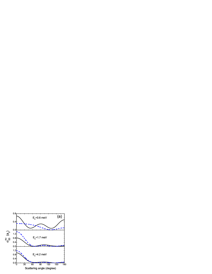
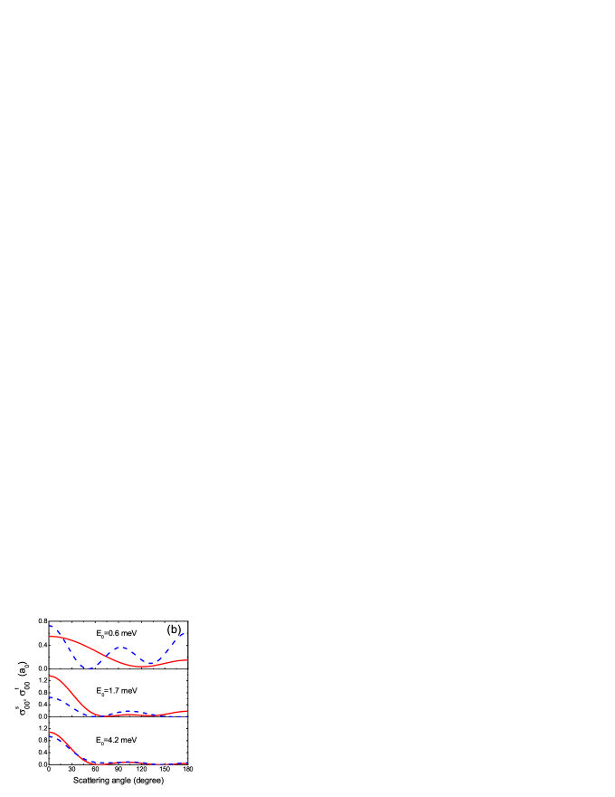
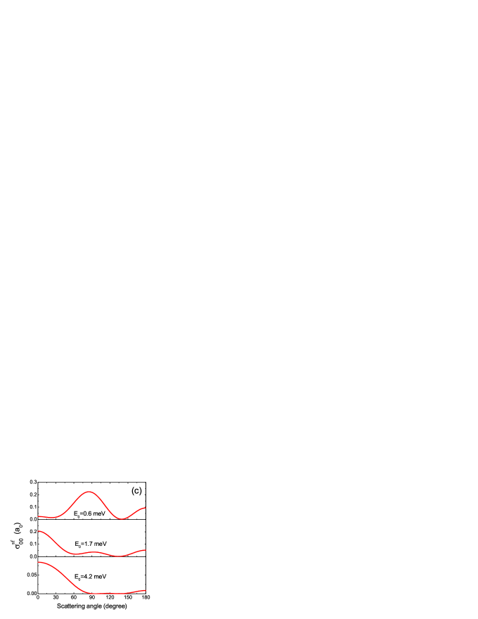
Figure 1: (Color online) The elastic DCS’s obtained within the one-channel model for electron scattering by the one-electron QD of $\hbar\omega_{0}=5$ meV and $r_{0}=35$ nm. The incident electron energies are indicated in the figures. (a) The spin-unpolarized DCS with (the solid curves) and without (the dashed curves) the exchange potential; (b) The DCS due to the singlet state (the solid curves) and the triplet state (the dashed curves); and (c) The spin-flip DCS.

IV.1 Convergency of the MCF

The MCF was applied to the electron-atom scatteringlee and electron-molecule scattering lee1 . In all those cases, it has shown a rapid convergency. Here, we apply the MCF to the electron-QD scattering in a two-dimensional semiconductor nanostructure. First of all, we check the convergency of this method for electron scattering through a QD. We consider a one-electron QD with $\hbar\omega_{0}=5$ meV, $r_{0}=35$ nm and an incident electron of kinetic energy $E_{0}=\hbar^{2}k_{0}^{2}/2m^{*}=$ 0.6 meV. The results are obtained within the one-channel approximation. For simplicity, only the static scattering potential is considered and the exchange potential is neglected in Eq. (III.2). Table I gives the calculated partial wave phase-shifts, for angular momenta up to $l=4$, of the first six iterations. Because the localization length of the confined electron wave-function in the QD is about $a_{0}=\sqrt{\hbar/m^{*}\omega_{0}}$, the screening parameter is taken as $\lambda=a_{0}^{-1}$ throughout this paper. ($a_{0}=14.75$ nm for a GaAs QD of $\hbar\omega_{0}=5$ meV). We have performed calculations with different values of $\lambda$. The calculated results have showed that, although a smaller $\lambda$ has enhanced the static potential scattering, the exchange effects and the spin-flip scattering are not affected significantly. From Table I we can see that the phase-shifts converge at the fifth iteration. It also shows that the first Born approximation, which corresponds to our zero-th iteration calculation, is indeed a very poor approximation in dealing with the electron-QD scattering. In order to obtain a correct scattering cross-section through a QD, it is necessary to use a robust method such as the MCF. Although the results in Table I are for a particular case, we have verified that all our calculations (with or without exchange interaction) in the present paper are convergent within 6 iterations.

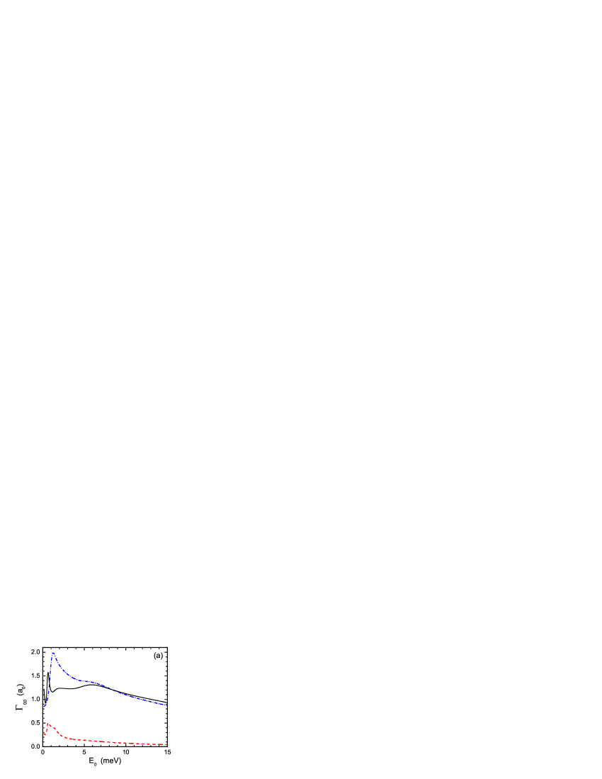
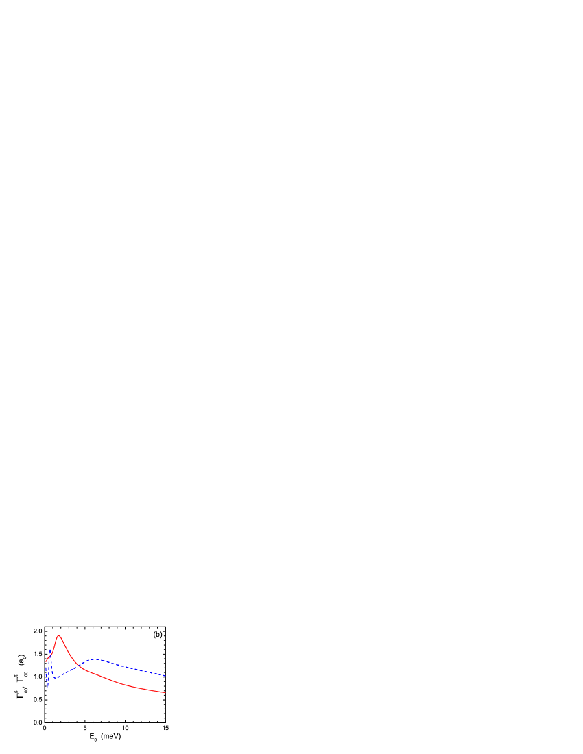
Figure 2: (Color online) The elastic ICS as a function of $E_{0}$ for the one-electron QD. (a) The su-ICS (the solid curve), the sf-ICS (the dashed curve), and the ICS due to the static potential only (the dotted-dash curve); (b) The ICS due to the singlet (the solid curve) and triplet states (the dashed curve) during the scattering.

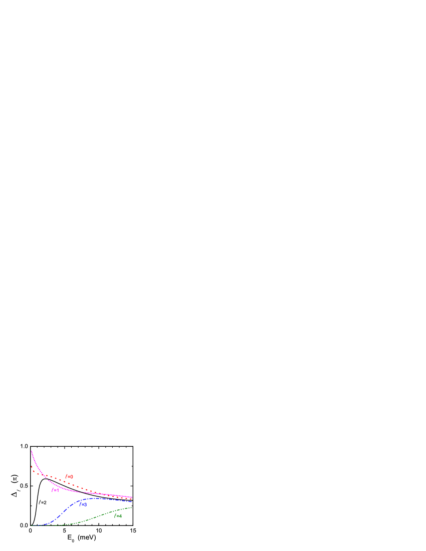
Figure 3: (Color online) The phase-shift as a function of $E_{0}$ for the partial waves $l=0$, 1, 2, 3, and 4 due to the static potential scattering of the one-electron QD.

IV.2 One-channel scattering

Within the one-channel approximation, we calculated the elastic DCS for electron scattering by the one-electron QD of $\hbar\omega_{0}=5$ meV and $r_{0}=$35 nm at incident kinetic energies $E_{0}=$0.6, 1.7, and 4.2 meV. The obtained DCS’s are presented in Fig. 1 as a function of the scattering angle. Fig. 1(a) shows the total or the su-DCS $\sigma^{\rm su}_{00}(\theta)$. To illustrate the effect of exchange interaction, the su-DCS’s due to the static potential only (i.e., neglecting the exchange potential in Eqs. (24) and (III.2)) are given by the dashed curves in the figure. We see that the exchange interaction is of significant contribution to the low-energy and/or small angle scattering. The exchange effect on the scattering is originated from the two different coupling states between the incident and the QD electrons (i.e., the singlet and the triplet states) during the collision as indicated in Eq. (24). The corresponding DCS’s due to the singlet [$\sigma^{{\rm s}}_{00}(\theta)$] and triplet states [$\sigma^{{\rm t}}_{00}(\theta)$] defined by Eqs. (29) and (30), respectively, are shown in Fig. 1(b). In Fig. 1(c), we plot the spin-flip (sf) DCS $\sigma^{{\rm sf}}_{00}(\theta)$ given by Eq. (33). Comparing Fig. 1(a) with Fig. 1(b), one can see that the exchange interaction affects more strongly the su-DCS when the difference between $\sigma^{{\rm s}}_{00}(\theta)$ and $\sigma^{{\rm t}}_{00}(\theta)$ is large. In Fig. 1(c) we observe that the spin-flip scattering due to exchange potential occurs mostly around $\theta\sim 90^{o}$ at lower incident energy ($E_{0}=$0.6 meV). For higher energies ($E_{0}=$1.7 and 4.2 meV), the spin-flip scattering is more relevant at small scattering angles.

Fig. 2(a) shows the ICS as a function of incident electron energy $E_{0}$ for the spin-unpolarized scattering and for that considering the static potential only. We see that the exchange interaction affects significantly the ICS at low $E_{0}$. At higher energies, however, the ICS is dominated by the static potential. In Fig. 2(a) we also present the spin-flip ICS (the dashed curve). A maximum spin-flip probability is found at $E_{0}=$1.1 meV which is about $37\%$ of the total scattering. In Fig. 2(b), we plot the ICS due to the singlet and the triplet states. It shows a strong dependence of the ICS on the spin states of two electrons in the system.

The scattering peaks in ICS due to the static potential (the dotted-dash curve in Fig. 2(a)) at $E_{0}=1.22$ and 6.0 meV are due to the occurrence of the so-called shape resonances, resulting from a virtual confined state at the corresponding energy. In order to clarify the origin of these features, we plot in Fig. 3 the corresponding partial wave phase-shifts $\Delta_{l}$ (for $l=0$, 1, 2, 3 and 4) due to the static potential. At $E_{0}\to 0$, $\Delta_{0}$ and $\Delta_{1}$ are larger than $\pi/2$ indicating the presence of the bound states of angular momenta $l=$0 and 1 in the QD. A rapid increase of $\Delta_{2}$ ($\Delta_{3}$) at around $E_{0}=1.2$ meV (6.0 meV) corresponds to a virtual bound state of $l=2$ ($l=3$) leading to the shape resonance scattering peak in the ICS. Similarly, peaks in the ICS at $E_{0}=1.72$ meV (0.57 meV) for the singlet (triplet) state scattering in Fig. 2(b) can be related to the virtual bound states in the system. The broad peak in the ICS of triplet state is possibly result from a virtual state of two interacting electrons.

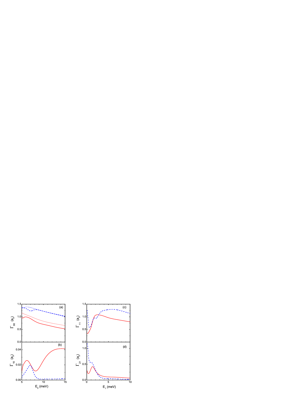
Figure 4: (Color online) The multichannel integral cross-sections $\Gamma^{\rm s}_{mi}$ (the solid curves) and $\Gamma^{\rm t}_{mi}$ (the dashed curves) as a function of $E_{i}$ ($i=0,1$) for the one-electron QD considering the three lowest energy states. The thin curves in (a) are the corresponding results within the one-channel model.

IV.3 Multi-channel scattering

The energy difference between the first excited state and the ground state is 4.90 meV in the QD of $\hbar\omega_{0}$=5 meV and $r_{0}$=35 nm. When the kinetic energy $E_{0}$ of an incident electron is higher than this energy difference, the inelastic scattering channel is open which leaves the QD in the excited state $\varepsilon_{1}$ after scattering. In such a case, the multichannel scattering process has to be considered. When the three lowest states of a one-electron QD are included in the calculation, there are 9 possible scattering channels. For the present QD, as the first excited state is two-fold degenerate, i.e. $\varepsilon_{1}=\varepsilon_{2}$, we find the following scattering cross-sections: the elastic $\Gamma_{00}(E_{0})$ and inelastic scattering $\Gamma_{10}(E_{0})$ for the QD initially in its ground state; the elastic scattering $\Gamma_{11}(E_{1})$ and super-elastic scattering $\Gamma_{01}(E_{1})$ for the QD initially in the first excited state. There are also two excitation cross-sections $\Gamma_{21}(E_{1})=\Gamma_{12}(E_{1})$ for the QD in the excited states of different angular momenta, although in these cases the energy of the scattered electron is the same as that of the elastic scattering $\Gamma_{11}(E_{1})$, i.e. $\varepsilon_{1}=\varepsilon_{2}$ and $k_{1}=k_{2}$ in Eq (27). In Fig. (4) we show the different integral cross-sections due to the singlet and the triplet states. Figs. 4(a) and 4(b) give the elastic ICS ($\Gamma_{00}$) and inelastic ICS ($\Gamma_{10}$), respectively, for the QD initially in its ground state. The inelastic cross-section is two orders of magnitude smaller than the elastic one. Moreover, the inelastic scattering due to the triplet state is very weak at higher energies. Coupling between different QD levels (or different scattering channels) leads to resonant scattering on both the elastic and inelastic cross-sections. The thin curves in Fig. 4(a) are the previous results in Fig. 2(b) of the ICS within the one-channel model. We see that the one-channel approximation yields quite good results for the elastic scattering.

Figs. 4(c) and 4(d) show the elastic ICS for the QD in the first excited state. At small incident energy $E_{1}$, the scattering due to the triplet state is much stronger than that due to the singlet state in this case. If the QD remains in the same excited state after the scattering, the ICS $\Gamma_{11}$ (=$\Gamma_{22}$) as shown in Fig. 4(c) is large at higher energy and decreases slowly with increasing $E_{1}$. However, if the angular momentum changes after the scattering, the ICS $\Gamma_{21}$ (=$\Gamma_{12}$) vanishes rapidly (both due to the singlet and triplet states) at high incident energies.

V Conclusion remarks

We presented a general method to calculate the electron scattering through an N-electron QD embedded in a two-dimensional semiconductor system. The multichannel L-S equations are solved numerically using the iterative method of continued fractions considering the electron-electron interactions. We applied this method to the case where only one electron is confined in the QD. The results indicate a rapid convergency of this method for two-dimensional scattering in a semiconductor nanostructure. It also shows that the first Born approximation is so poor that cannot yield correct scattering cross-section.

We found that the exchange effects are relevant when the kinetic energy of incident electron is small, as showed by the obtained DCS and ICS. The shape resonances were found in the elastic ICS including or not the exchange potential. The spin-flip cross-section due to exchange interaction shows a maximum both in the DCS as a function of the scattering angle and in the ICS as a function of the incident electron energy. The maximum spin-flip scattering reaches as high as more than 30% in comparison to the total scattering. In multichannel scattering including the excited states of the QD, we obtained the inelastic scattering cross-sections. They are about two orders of magnitude smaller than the elastic ones.

In this paper, we emphasize the theoretical approach and numerical method to calculate the electron scattering by a charged quantum dot. The scattering cross-sections were obtained for a spin unpolarized system. It can be extended to a spin polarized system which is of great interest for electron transport in semiconductor nanostructures. The application to a spin polarized system is straightforward as soon as the initial spin states of the system are defined. In the numerical calculation, we presented the cross-sections due to a one-electron QD scattering. For a QD of two or more electrons, we need firstly to know the eigenstates of the QD with electron-electron interactions. Then the scattering cross-sections can be calculated according to the total wavefunction defined by Eq. (6) as what has been done for electron-atom and electron-molecule scattering where several electrons are presented.lee1

Appendix A Method of Continued Fractions

The method of continued fractions (MCF)mcf is an iterative method to solve the L-S equation. To apply this method for a multi-channel scattering we have firstly to rewrite Eq. (12) in a matrix form:

$$\widetilde{\Psi}=\widetilde{\varphi}+\widetilde{G}^{(0)}\widetilde{V}\widetilde{\Psi}.$$ (36)

In the first step to start the MCF, we use the scattering potential $\widetilde{V}=V^{(0)}$ and the free electron wave-function $\widetilde{\varphi}=|\varphi^{(0)}\rangle$ in Eq. (36). Afterwards, we define the n$th$-order weakened potential as

$$V^{(n)}=V^{(n-1)}-\frac{V^{(n-1)}|\varphi^{(n-1)}\rangle\langle\varphi^{(n-1)}|V^{(n-1)}}{\langle\varphi^{(n-1)}|V^{(n-1)}|\varphi^{(n-1)}\rangle},$$ (37)

where

$$|\varphi^{(n)}\rangle=\widetilde{G}^{(0)}V^{(n-1)}|\varphi^{(n-1)}\rangle.$$ (38)

The n$th$-order correction of the T matrix can be obtained through

$$T^{(n)}=\langle\varphi^{(n-1)}|V^{(n-1)}|\varphi^{(n)}\rangle+\langle\varphi^{(n)}|V^{(n)}|\varphi^{(n)}\rangle$$

$$\times\left[\langle\varphi^{(n)}|V^{(n)}|\varphi^{(n)}\rangle-T^{(n+1)}\right]^{-1}\langle\varphi^{(n)}|V^{(n)}|\varphi^{(n)}\rangle.$$ (39)

Hence, we can stop the iteration when the potential $V^{(N)}$ becomes weaker enough. In the numerical calculation, we start with $T^{(N+1)}=0$ and evaluate $T^{(N)},T^{(N-1)},...,$ and $T^{(1)}$. Therefore the T matrix is given by

$$\mathbf{T}=\langle\varphi^{(0)}|V^{(0)}|\varphi^{(0)}\rangle+T^{(1)}\frac{\langle\varphi^{(0)}|V^{(0)}|\varphi^{(0)}\rangle}{\langle\varphi^{(0)}|V^{(0)}|\varphi^{(0)}\rangle-T^{(1)}}.$$ (40)

Appendix B Partial wave expansion

In two dimensions the angular momentum basis is given by2d ,

$$\Theta_{l}(\phi)=\sqrt{\frac{\kappa_{l}}{2\pi}}\cos(l\phi)$$ (41)

where $l=0,1,2,...$, $\kappa_{l}=2$ for $l\neq 0$ and $\kappa_{l}=1$ for $l=0$. In applying the partial wave expansion in the multi-channel scattering problem Eq. (12), we expand all functions, i.e., the incident free electron wavefunction $\varphi_{i}(\mathbf{r})$, the Green’s function $G^{(0)}(\mathbf{k}_{m},\mathbf{r},\mathbf{r^{\prime}})$, and the scattered electron wavefunction $\psi_{mi}(\mathbf{r})$, in the angular momentum basis as follows,

$$\varphi_{i}(\mathbf{r})=\sum_{l,l^{\prime}=0}^{\infty}\sqrt{\frac{\kappa_{l}}{2\pi}}i^{l}J_{l}(kr)\delta_{ll^{\prime}}\Theta_{l}(\phi_{r})\Theta_{l^{\prime}}(\phi_{k}),$$ (42)

and

$$\psi_{mi}(\mathbf{r})=\sum_{l,l^{\prime}=0}^{\infty}\psi_{mi}^{l,l^{\prime}}(k,r)\Theta_{l}(\phi_{r})\Theta_{l^{\prime}}(\phi_{k}),$$ (43)

where $\phi_{r}$ and $\phi_{k}$ are the variables due to expansion on the position $\bf r$ and momentum ${\bf k}$, respectively. The expansion on the Green’s function yields the following expression,

$$G^{(0)}(\mathbf{k}_{m},\mathbf{r},\mathbf{r^{\prime}})=$$ (44)

$$-\frac{i\pi}{2}\sum_{l=0}^{\infty}\sqrt{\frac{\kappa_{l}}{2\pi}}J_{l}(k_{m}r_{<})H^{(1)}_{l}(k_{m}r_{>})\Theta_{l}(\phi_{r})\Theta_{l}(\phi_{r^{\prime}}),$$

where $k=k_{i}$, $r_{<}={\rm min}(r,r^{\prime})$, $r_{>}={\rm max}(r,r^{\prime})$, $J_{l}(k_{m}r)$ ($Y_{l}(k_{m}r$)) is the Bessel (Neumann) function and $H^{(1)}_{l}(k_{m}r)=J_{l}(k_{m}r)+iY_{l}(k_{m}r)$ is the Hankel function morse . Using the partial wave expansion the Lippmann-Schwinger equation can be reduced to a set of radial equations. The radial Lippmann-Schwinger equation corresponding to Eq. (12) is given by,

$$\psi_{mi}^{l,l^{\prime}}(k,r)=\sqrt{\frac{\kappa_{l}}{2\pi}}i^{l}J_{l}(kr)\delta_{ll^{\prime}}\delta_{mi}$$ (45)

$$+\sum_{l^{\prime\prime}=0}^{\infty}\sum_{n=0}^{\infty}\int_{0}^{\infty}r^{\prime}dr^{\prime}g^{l}_{0}(k_{m},r,r^{\prime})V_{mn}^{l,l^{\prime\prime}}(r^{\prime})\psi_{ni}^{l^{\prime\prime},l^{\prime}}(r^{\prime}),$$

where

$$g^{l}_{0}(k_{m},r,r^{\prime})=\frac{-i\pi}{2}\sqrt{\frac{\kappa_{l}}{2\pi}}J_{l}(k_{m}r_{<})H^{(1)}_{l}(k_{m}r_{>})$$ (46)

and

$$V^{l,l^{\prime\prime}}_{mn}(r^{\prime})=\int_{0}^{2\pi}d\phi_{r^{\prime}}\Theta_{l}(\phi_{r^{\prime}})V_{mn}(\mathbf{r^{\prime}})\Theta_{l^{\prime\prime}}(\phi_{r^{\prime}}).$$ (47)

We see that, when the partial wave method is used, there is a change in the continuum variable $\phi$ to a partial wave $l$. Consequently, the wavefunction $\psi_{mi}(\mathbf{r})$ becomes a matrix function with elements $\psi^{l,l^{\prime}}_{mi}(k,r)$.

The partial wave expansion for the exchange potential is a little subtle due to its non-locality. Here, we show some details how the partial wave expansion is applied in this case. We take as an example the exchange potential which couples the channels $n$ and $m$ for a single electron spin-orbital $\alpha$,

$$V_{mn}^{\rm ex}(\mathbf{r})\psi_{ni}(\mathbf{r})=-\frac{e^{2}}{\epsilon^{*}_{0}}\zeta^{n}_{\alpha}(\mathbf{r})\int d\mathbf{r_{1}}\zeta_{\alpha}^{m*}(\mathbf{r_{1}})\frac{1}{|\mathbf{r}-\mathbf{r_{1}}|}\psi_{ni}(\mathbf{r_{1}}).$$ (48)

The partial wave expansion of the spin-orbital function is given by

$$\zeta^{n}_{\alpha}(\mathbf{r})=\sum_{l=0}^{\infty}\zeta^{l}_{n\alpha}(r)\Theta_{l}(\phi_{r}).$$ (49)

The product of two different functions can also be expanded in the angular momentum basis as follows,

$$\psi_{ni}(\mathbf{r})\zeta^{m*}_{\alpha}(\mathbf{r})=\sum_{l,l^{\prime}}\Pi_{ni;m\alpha}^{l,l^{\prime}}(r)\Theta_{l}(\phi_{r})\Theta_{l^{\prime}}(\phi_{k}),$$ (50)

where

$$\Pi_{ni;m\alpha}^{l,l^{\prime}}(r)$$ (51)

$$=\sum_{\lambda,\lambda^{\prime}}\frac{\psi_{ni}^{\lambda,l^{\prime}}(k,r)\zeta^{\lambda^{\prime}*}_{m\alpha}(r)}{2\sqrt{2\pi}}\sqrt{\frac{\kappa_{\lambda}\kappa_{\lambda^{\prime}}}{\kappa_{l}}}\left(\delta_{l,\lambda+\lambda^{\prime}}+\delta_{l,|\lambda-\lambda^{\prime}|}\right).$$

Using the above relation, we obtain Eq. (48) in the partial wave expansion form,

$$V_{mn}^{\rm ex}(\mathbf{r})\psi_{ni}(\mathbf{r})=-\frac{e^{2}}{\epsilon^{*}_{0}}\zeta^{n}_{\alpha}(\mathbf{r})\sum_{l,l^{\prime}}\Theta_{l}(\phi_{r})\Theta_{l^{\prime}}(\phi_{k})$$ (52)

$$\times\int_{0}^{\infty}r_{1}dr_{1}\Pi_{ni;m\alpha}^{l,l^{\prime}}(r_{1})\int_{0}^{2\pi}\frac{\Theta_{l}(\theta)d\theta}{\sqrt{r^{2}+r_{1}^{2}-2rr_{1}\cos(\theta)}},$$

where $\theta=\phi_{r}-\phi_{r_{1}}$. To solve the angular integral we use the generating function of the Legendre Polynomialsmorse ,

$$\frac{1}{\sqrt{r^{2}+r_{1}^{2}-2rr_{1}\cos(\theta)}}=\sum_{j=0}^{\infty}\frac{r_{<}^{j}}{r_{>}^{j+1}}P_{j}(\cos\theta),$$ (53)

where $r_{<}={\rm min}(r,r_{1})$, $r_{>}={\rm max}(r,r_{1})$ and $P_{j}(\cos\theta)$ are the Legendre Polynomials. Thus the angular integral that we need to solve is

$$c_{l,j}=\int_{0}^{2\pi}d\theta\Theta_{l}(\theta)P_{j}(\cos\theta).$$ (54)

Substituting the Eqs. (53) and (54) into Eq. (52) we obtain finally the exchange potential

$$V_{mn}^{\rm ex}(\mathbf{r})\psi_{ni}(\mathbf{r})=-\frac{e^{2}}{\epsilon^{*}_{0}}\zeta^{n}_{\alpha}(\mathbf{r})\sum_{l,l^{\prime}}\Theta_{l}(\phi_{r})\Theta_{l^{\prime}}(\phi_{k})\times$$

$$\times\sum_{j=0}^{\infty}\int_{0}^{\infty}r_{1}dr_{1}\Pi_{ni;m\alpha}^{l,l^{\prime}}(r_{1})c_{l,j}\frac{r_{<}^{j}}{r_{>}^{j+1}}.$$ (55)

In the numerical calculations, we firstly evaluate the coefficients $c_{l,j}$ given by Eq. (54). Then the integration on $r_{1}$ in Eq. (55) is performed for each iteration in the MCF. Finally we multiply the result by $-\frac{e^{2}}{\epsilon^{*}_{0}}\zeta^{n}_{\alpha}(\mathbf{r})$.

Within the one-channel approximation ($i=m=n=0$), the calculations can be further simplified by using the concept of phase shift. Considering a central potential $V(r)$ ($l=l^{\prime}=l^{\prime\prime}$), Eq. (45) becomes

$$\psi^{l}(k,r)=\sqrt{\frac{\kappa_{l}}{2\pi}}i^{l}J_{l}(kr)+\int_{0}^{\infty}r^{\prime}dr^{\prime}g^{l}_{0}(k,r,r^{\prime})V(r^{\prime})\psi^{l}(k,r^{\prime})$$ (56)

where $\psi^{l}(k,r)=\psi^{l,l}_{00}(k,r)$. To define the phase-shift we write the asymptotic form of the above equation as

$$\psi^{l}(k,r)\hbox{ \raise-5.69054pt\hbox{$\textstyle\longrightarrow\atop\scriptstyle r\rightarrow\infty$} }A_{l}\sqrt{\frac{1}{kr}}\cos(kr-\frac{l\pi}{2}-\frac{\pi}{4}-\Delta_{l}),$$ (57)

where $\Delta_{l}$ is the phase-shift. Comparing the coefficients of $e^{ikr}$ and $e^{-ikr}$ of Eq. (57) with the asymptotic form of Eq. (56) one can obtain the following relations

$$A_{l}=2\sqrt{\frac{\kappa_{l}}{\pi}}i^{l}e^{i\Delta_{l}},$$ (58)

and

$$e^{i\Delta_{l}}\sin\Delta_{l}=\frac{-\pi}{2i^{l}}\int_{0}^{\infty}r^{\prime}dr^{\prime}J_{l}(kr^{\prime})V(r^{\prime})\psi^{l}(r^{\prime}).$$ (59)

On the other hand, from the definition of the scattering amplitude in Eq. (14), we can express the scattering amplitude $f_{k_{0},k_{0}}$ in terms of the phase-shift2d $\Delta_{l}$,

$$f_{k_{0},k_{0}}(\theta)=2\sum_{l=0}^{\infty}\sqrt{\frac{\kappa_{l}}{\pi}}e^{i\Delta_{l}}\sin\Delta_{l}\Theta_{l}(\theta).$$ (60)

The corresponding DCS is $\sigma_{00}(\theta)=\left|f_{k_{0},k_{0}}(\theta)\right|^{2}/k$ and the ICS is given by

$$\Gamma_{00}=\frac{4}{k}\sum_{l=0}^{\infty}\kappa_{l}\sin^{2}\Delta_{l}.$$ (61)

References

- (1) F. H. L. Koppens, C. Buizert, K. J. Tielrooij, I. T. Vink, K. C. Nowack, T. Meunier, L. P. Kowenhoven, and L. M. K. Vandersypen, Nature 442, 766 (2006).
- (2) F. Y. Qu and P. Vasilopoulos, Phys. Rev. B 74, 245308 (2006).
- (3) J. Fransson, E. Holmström, O. Eriksson, and I. Sandalov, Phys. Rev. B 67, 205310 (2003).
- (4) J. König and J. Martinek, Phys. Rev. Lett. 90, 166602 (2003).
- (5) P. Zhang, Q.-K. Xue, Y. Wang, and X. C. Xie, Phys. Rev. Lett. 89, 286803 (2002).
- (6) H.-A. Engel and D. Loss, Phys. Rev. B 65, 195321 (2002).
- (7) P. Seneor, A. Bernand-Mantel, and F. Petroff, J. Phys.: Condens. Matter 19, 165222 (2007).
- (8) S. A. Wolf, D. D. Awschalom, R. A. Buhrman, J. M. Daughton, S. von Molnár, M. L. Roukes, A. Y. Chtchelkanova, and D. M. Treger, Science 294, 1488 (2001).
- (9) G. Burkard, H. A. Engel, and D. Loss, Fortschr. Phys. 48, 965 (2000).
- (10) S. Das Sarma, J. Fabian, X. Hu, and I. Zutic, Solid State Commun. 119, 207 (2001).
- (11) K. Gündogdu, K. C. Hall, T. F. Boggess, D. G. Deppe, and O. B. Shchekin, Appl. Phys. Lett. 84, 2793 (2004).
- (12) F. Buscemi, P. Bordone, and A. Bertoni, Phys. Rev. A 73, 052312 (2006).
- (13) T. Ji, Q. F. Sun, and H. Guo, Phys. Rev. B 74, 233307 (2006).
- (14) A. Pályi, C. Péterfalvi, and J. Cserti, Phys. Rev. B 74, 073305 (2006).
- (15) C. J. Joachain, “Quantum Collision Theory”, North-Holland, (Amsterdam, 1975).
- (16) B. H. Bransden and M. R. C. McDowell, Phys. Rep. 30, 207 (1977).
- (17) J. Horáček and T. Sasakawa, Phys. Rev. A 28, 2151 (1983); 30, 2274 (1984).
- (18) M.-T. Lee, I. Iga, M. M. Fujimoto, and O. Lara, J. Phys. B 28, L299 (1995).
- (19) A. M. Machado, M. M. Fujimoto, A. M. Taveira, L. M. Brescansin, and M.-T. Lee, Phys. Rev. A 63, 032707 (2001); E. M. S. Ribeiro, L. E. Machado, M.-T. Lee, and L. M. Brescansin, Comput. Phys. Commun. 136, 117 (2001).
- (20) A. Szabo and N. Ostlund, “Modern Quantum Chemistry”, Macmillan Publishing , (New York, 1982).
- (21) P. M. Morse and H. Feshbach, “Methods of Theoretical Physics”, McGraw-Hill, (New York, 1953).
- (22) S. K. Adhikari, Am. J. Phys. 54, 362 (1986).
- (23) V. Fock, Z. Phys. 47, 446 (1928); C. Darwin, Proc. Cambridge Philos. Soc. 27, 86 (1930).