Supernovae in the Subaru Deep Field:
An Initial Sample, and Type Ia Rate, out to Redshift 1.6

Abstract

Large samples of high-redshift supernovae (SNe) are potentially powerful probes of cosmic star formation, metal enrichment, and SN physics. We present initial results from a new deep SN survey, based on re-imaging in the $R,~{}i^{\prime},~{}z^{\prime}$ bands, of the $0.25~{}\mathrm{deg}^{2}$ Subaru Deep Field (SDF), with the 8.2 m Subaru telescope and Suprime-Cam. In a single new epoch consisting of two nights of observations, we have discovered 33 candidate SNe, down to a $z^{\prime}$-band magnitude of 26.3 (AB). We have measured the photometric redshifts of the SN host galaxies, obtained Keck spectroscopic redshifts for 17 of the host galaxies, and classified the SNe using the Bayesian photometric algorithm of Poznanski et al. (2007) that relies on template matching. After correcting for biases in the classification, 55% of our sample consists of Type Ia supernovae and 45% of core-collapse SNe. The redshift distribution of the SNe Ia reaches $z\approx 1.6$, with a median of $z\approx 1.2$. The core-collapse SNe reach $z\approx 1.0$, with a median of $z\approx 0.5$. Our SN sample is comparable to the Hubble Space Telescope/GOODS sample both in size and redshift range. The redshift distributions of the SNe in the SDF and in GOODS are consistent, but there is a trend (which requires confirmation using a larger sample) for more high-$z$ SNe Ia in the SDF. This trend is also apparent when comparing the SN Ia rates we derive to those based on GOODS data. Our results suggest a fairly constant rate at high redshift that could be tracking the star-formation rate. Additional epochs on this field, already being obtained, will enlarge our SN sample to the hundreds, and determine whether or not there is a decline in the SN Ia rate at $z\gtrsim 1$.

1 Introduction

Supernovae (SNe) hold the key to several open astrophysical questions. In particular, SNe are the main source of heavy elements, and their energy input to the interstellar medium (ISM) is a vital ingredient in galaxy formation (e.g., Yepes et al. 1997). Learning the nature of the progenitors of different SN types, the SN rates, and the SN distributions in both space and cosmic time, are essential steps toward understanding metal enrichment and galaxy formation (e.g., Kobayashi, Tsujimoto & Nomoto 2000), and will be a prime topic of study with the James Webb Space Telescope.

It is widely believed that SNe Ia arise from the explosions of white dwarfs (WDs) in binary systems, while all other SN types result from massive-star core collapse (e.g., Filippenko 1997; Gal-Yam et al. 2007; Li et al. 2007, and references therein). Core-collapse SNe (CC-SNe) therefore explode promptly ($\lesssim 10$ Myr) after the formation of a stellar population, and the CC-SN rate will trace the star-formation history (SFH). In contrast, SNe Ia should occur only after WD formation and binary evolution, with a “delay” of order 0.1–10 Gyr. The SN Ia rate vs. cosmic time will therefore be a convolution of the SFH with a “delay function” — the SN Ia rate following a brief burst of star formation.

The progenitors of SNe Ia have not been identified, and could be WDs accreting from main-sequence companions, sub-giants, or giants, or alternatively “double-degenerate” WD pairs that merge (e.g., Hillebrandt & Niemeyer 2000, and references therein). Each of these scenarios predicts a different delay function (e.g., Kobayashi et al. 1998; Madau, Della Valle & Panagia 1998; Yungelson & Livio 1998; Belczynski, Bulik & Ruiter 2005; Greggio 2005; see recent updates in Panagia, Della Valle & Mannucci 2007), which in turn dictates the SN rate vs. redshift. For the local Universe, current estimates of SN rates (e.g., Cappellaro, Evans & Turatto 1999; Mannucci et al. 2005; Sharon et al. 2007) are still uncertain, but improving substantially (Leaman, Li, & Filippenko 2007, in preparation). At $z\approx 0.3-1.6$, a number of sometimes conflicting measurements exist (Pain et al. 2002; Gal-Yam, Maoz & Sharon 2002; Tonry et al. 2003; Dahlen et al. 2004; Cappellaro et al. 2005; Barris & Tonry 2006; Neill et al. 2006; Sullivan et al. 2006b).

Recent attempts to constrain the cosmic SFH and the SN Ia delay function using SN rates have yielded some intriguing results. Gal-Yam et al. (2002) carried out the first measurement of cluster SN Ia rates at $z=0.25$ and $z=0.9$ using deep ($R\approx 27$ mag) archival Hubble Space Telescope (HST) images of eight massive clusters. In Maoz & Gal-Yam (2004), the measured rates were compared to predictions normalized by the requirement that SNe Ia produce the observed mass of iron in clusters. The low observed rate at $z\approx 1$ implies that the SNe needed to produce the iron exploded at earlier times, arguing against models with long SN Ia time delays, which predict SN rates ten times higher than observed. Thus, cluster iron production by SNe Ia appeared to be a viable option only if SNe Ia have relatively short ($\lesssim 2$ Gyr) time delays. In contrast, comparison of the SN Ia rate vs. $z$ in the field to the cosmic SFH has generally suggested a long delay time (Pain et al. 2002; Tonry et al. 2003; Gal-Yam & Maoz 2004; Strolger et al. 2004; see, however, Barris & Tonry 2006, who find evidence for a short delay). These results may therefore point to CC-SNe from an early generation of star formation with a top-heavy initial mass function, rather than SNe Ia, as the source of cluster enrichment.

However, a re-analysis by Förster et al. (2006) of the HST-based Great Observatories Origins Deep Survey (GOODS) data of Strolger et al. (2004), originally obtained to measure the expected early deceleration of the Universe (Riess et al. 2004a), indicates that these conclusions may be strongly dependent on the assumed SFH. Furthermore, evidence has surfaced that there may be two separate SN Ia channels, a “prompt” ($\sim 1$ Gyr) channel and a “tardy” ($\sim 10$ Gyr) one (Mannucci et al. 2005; Scannapieco & Bildsten 2005; Mannucci, Della Valle & Panagia 2006). A single delay distribution that is peaked at short delays but includes a long tail extending to large delays may be able to reproduce most of the current data. Nevertheless, some rate measurements at similar redshifts are discrepant by large factors (e.g., Pain et al. 2002 vs. Barris & Tonry 2006). There is ongoing debate as to whether incompleteness or contamination of SN samples are affecting the low or high-rate measurements, respectively. The decrease in the field SN Ia rate at $z>1$ measured by Dahlen et al. (2004) and Strolger et al. (2004), if real, does not permit the existence of the prompt SN Ia component indicated by the high SN Ia rate seen in star-forming galaxies (Mannucci et al. 2005, 2006; Sullivan et al. 2006b). Scannapieco & Bildsten (2005) have actually predicted that this apparent decrease will disappear with improved data. Barris & Tonry (2006) have argued that the claims for long delay times depend strongly on the presence of very few SNe at the highest redshifts in the GOODS survey. Indeed, small-number statistics are a major limiting factor in all current estimates of SN rates at high $z$. Progress in this field requires larger high-$z$ SN samples than presently available.

However, with typical magnitudes of $\sim$25–26, samples of high-$z$ SNe are currently difficult to confirm (or classify) spectroscopically. Photometric classification of SNe has been shown do be a viable option by Poznanski et al. (2002), and further explored since then (e.g., Gal-Yam et al. 2004b; Riess et al. 2004b; Sullivan et al. 2006a). Recently, Poznanski, Maoz & Gal-Yam (2007, hereafter P07) have developed an automatic Bayesian algorithm for the purpose of classifying SNe with single-epoch photometry. The major novelties in the approach of P07 lie in the probabilistic classification, and the ability to quantify the success fractions, uncertainties, and biases of photometric SN typing. This opens the possibility for surveys for large numbers of SNe, and their classification, using solely single-epoch, ground-based, imaging.

In this paper, we present initial results from a survey in which we attempt this new approach for obtaining large high-$z$ SN samples. The survey is conducted by re-imaging the Subaru Deep Field (SDF; Kashikawa et al. 2004, hereafter K04) in three bands. Keck spectroscopy of over half of the SN hosts, and for several hundred galaxies similar to the hosts, is used to estimate the reliability of our photometric redshifts. The photometry of the SNe and their hosts is used to classify the SNe with the algorithm of P07. As we show below, we identify 33 SNe, classified as either Type Ia or core collapse, with redshifts out to $\sim 1.7$, a number and redshift range comparable to those in the HST/GOODS sample. While the redshift distributions of the samples are consistent, there is a trend for more high-$z$ SNe Ia in the SDF. We derive the SN Ia rate, in four redshift bins, and find that while it is consistent, to within errors, with previous results, at redshift $z\approx 1.6$ it is about 50% higher than the value determined based on GOODS data, and at redshift $z\approx 0.7$ the rate we find is lower than that of GOODS. We are currently in the process of increasing our SN sample by obtaining additional epochs of the SDF, with the objective of acquiring a sample of several hundred high-$z$ SNe. Those observations and their analysis will be described in future papers.

2 Observations and Reductions

2.1 Imaging

Our SN survey is carried out in the SDF ($\alpha=13^{h}24^{m}39^{s}$, $\delta=+27^{\circ}29^{\prime}26^{\prime\prime}$; J2000). The reference images for this field, obtained with the Suprime-Cam camera on the Subaru 8.2-m telescope on Mauna Kea, Hawaii, are described by K04. Suprime-Cam is a $5\times 2$ mosaic of $2{\rm k}\times 4{\rm k}$ CCDs at the prime focus of the telescope, with a field of view of $34\arcmin\times 27\arcmin$, and a scale of $0\aas@@fstack{\prime\prime}202~{}\textrm{pixel}^{-1}$. This reference epoch of the SDF was obtained by deep imaging, in five broad-band filters ($B,V,R,i^{\prime},~{}\mathrm{and}~{}z^{\prime}$) and two narrow-band filters ($NB816$ and $NB921$), of an area of $30\arcmin\times 37\arcmin$, down to $3\sigma$ limiting magnitudes of $B=28.45$, $V=27.74$, $R=27.80$, $i^{\prime}=27.43$, and $z^{\prime}=26.62$ ($5\sigma$ limits of $B=28.06$, $V=27.33$, $R=27.37$, $i^{\prime}=27.13$, and $z^{\prime}=26.32$; here and throughout the paper, all magnitudes are on the AB system; Oke & Gunn 1983). The imaging for the reference SDF epoch was carried out between April 2002 and April 2003, with some preliminary data collected in 2001, as described by K04.

We re-imaged the field on 2005 March 5 and 6 (UT dates are used throughout this paper), in the three reddest Suprime-Cam broad bands: $R$, $i^{\prime}$, and $z^{\prime}$. These bands were selected as being the most efficient for finding high-redshift SNe, and for later classification (e.g., Poznanski et al. 2002; Gal-Yam et al. 2004b; Riess et al. 2004b). We obtained 22 exposures of $360$ s each in $R$, 36 of $300$ s each in $i^{\prime}$, and 76 of $240$ s each in $z^{\prime}$, for a total of $7920$ s ($R$), $10,800$ s ($i^{\prime}$), and $18,240$ s ($z^{\prime}$). We followed a dithering pattern similar to the one described by K04. Our seeing throughout the observations averaged $0\aas@@fstack{\prime\prime}65$ in all three bands, ranging from $0\aas@@fstack{\prime\prime}5$ to $0\aas@@fstack{\prime\prime}8$.

We also observed the field with the MOSAIC-I wide-field imager on the Kitt Peak National Observatory (KPNO) 4-m Mayall telescope, on 2005 March 2, April 5, and June 8, and on 2006 June 19. The MOSAIC-I camera consists of eight CCDs with a pixel size of $0\aas@@fstack{\prime\prime}258$ (Muller et al. 1998), covering a field of view of $36\arcmin\times 36\arcmin$. Each observation was in white light (i.e., unfiltered), typically 1.5–2 hr long, split into dithered subexposures, with a median seeing of about $0\aas@@fstack{\prime\prime}8$. Compared to the $R$ band, the unfiltered observations increase the throughput of stellar sources, depending on their colours, by a factor of 2–4, and also increase the level of the sky background by a factor of 4–8, depending on conditions. The signal-to-noise ratio (S/N) is therefore multiplied by $(2-4)\,/\,\sqrt{4-8}\approx(0.7-2)$. Consequently, in many cases, unfiltered observations permit obtaining a deeper image, closer to the depth reached with the larger-aperture Subaru telescope, albeit with no colour information. The 4-m data provide us with monitoring over longer times, which is important for identifying variable active galactic nuclei (AGNs), the main contaminant in our SN search (see §3).

The HST archive includes Advanced Camera for Surveys (ACS) images of a small portion of the SDF, which we use to examine the morphology of one SN host galaxy that lies in this field. The data were obtained with HST/ACS in 2002, on five separate occasions between May 20 and July 3, in the F850LP band as part of program GO-9075 (PI: S. Perlmutter). The total exposure time is $5370$ s.

Subaru data were reduced following K04, using the Suprime-Cam pipeline SDFRED (Yagi et al. 2002; Ouchi et al. 2004), and involving the following main steps. The individual frames were overscan subtracted, flat fielded using superflats, distortion corrected, matched to a common point-spread function (PSF) of $0\aas@@fstack{\prime\prime}98$, sky subtracted, registered, and combined. The combined image was then matched to the reference image by using the astrometrix code to find the astrometric correction, and the IRAF (Tody 1986) task wregister was used to register the two images. Inducing PSF degradation to the new images may appear questionable, since it reduces the frame depth and could adversely affect the subsequent image subtraction. However, probably because our reference epoch was reduced in such a manner, we found that the optimal image subtraction, with the least numbers of artificial residuals, was obtained by following the same procedure. The photometric calibration of the first-epoch images was done by K04, reaching a precision for the zero points of about 0.05 mag. We calibrated our images relative to the first epoch by comparing the photometry of all the objects detected in both epochs. The mean of the differences between the two measurements was taken to be the difference in zero points. The final images reach $3\sigma$ limits (defined as in K04) of $R=27.4$, $i^{\prime}=27.1$, and $z^{\prime}=26.3$ ($5\sigma$ limits of $R=26.9$, $i^{\prime}=26.7$), and $z^{\prime}=26.0$), shallower than the reference image by $0.5$ mag ($R$), $0.4$ mag ($i^{\prime}$), and $0.4$ mag ($z^{\prime}$).

Reduction of the KPNO images was done using the IRAF package MSCRED, following the same steps as with the Subaru data, except that PSF degradation was not applied. The final images reach $3\sigma$ limiting magnitudes corresponding approximately to $R=25-26$ mag ($5\sigma$ limits of $R=24.5-25.3$ mag), depending on the epoch. The depth reached implies a S/N improvement in the filterless data, relative to $R$-band imaging, of a factor near 2, for two of our epochs, and only a minor gain for the remaining two. HST images were reduced using the PyRAF script MultiDrizzle (Koekemoer et al. 2002).

We performed PSF matching and image subtraction between the new and reference Subaru images in all bands, and between the four KPNO epochs, using both the software ISIS (Alard & Lupton 1998; Alard 2000) and the Common PSF Method (CPM; Gal-Yam et al. 2004a; Gal-Yam et al. 2007, in preparation). Briefly, ISIS minimizes a spatially variable convolution kernel that degrades the PSF of the better-seeing image to the PSF of the worse-seeing image. CPM convolves each image with the measured PSF of the other, and thus the final PSF of both images is worse than the initial PSF of either image, but kernel-matching, and its inherent uncertainties in the presence of noise and pixellation, are avoided. Both procedures produce output images with nominally identical PSFs, while introducing a minimal amount of noise. While ISIS is robust and stable, we find that in some cases it tends to produce more subtraction artefacts than CPM, mimicking SNe near the cores of bright galaxies. We have therefore used both codes.

As a consequence of the dithering, the final images have a field of view of $0.31~{}\mathrm{deg^{2}}$, but with a substantial region along the edges where the S/N is significantly smaller. This is due to the different effective exposure on the fringes of the field. We therefore trim down the difference image to 81% of its full size, and remain with a total differenced area of $0.25~{}\mathrm{deg^{2}}$ (which is, in fact, the size of the Suprime-Cam field).

2.2 Spectroscopy

We obtained spectra of some of our SN host galaxies (see §4), and of several hundred random galaxies in the SDF. Observations were carried out on 2007 January 12, January 22, March 16, and April 12, using the Low-Resolution Imaging Spectrometer (LRIS; Oke et al. 1995) on the Keck I telescope for the first night, and the Deep Imaging Multi-Object Spectrograph (DEIMOS; Faber et al. 2003) on the Keck II telescope for the three other nights. Eight unique object masks and positions where used, with up to 12 host galaxies per mask (including also targets from Subaru observations in February 2007, which are not analysed in this paper), and several tens of random galaxies per mask. Each mask was typically observed for $3\times 1800$ s.

The LRIS mask was observed with the 600 line mm^-1 grism blazed at 4000 Å, and the 400 line mm^-1 grating blazed at 8500 Å, together with the D560 dichroic. This typically yields a wavelength range of $\sim$3000–10,000 Å, but the specific position of the slit on the mask shifts the wavelength range for each individual spectrum. The spectra have resolutions of $\sim$3.5 Å and $\sim$7.0 Å for the blue and red sides, respectively.

All but one of the DEIMOS masks were observed with the 600 line mm^-1 grating blazed at 7500 Å, and the GG495 order-blocking filter. We chose a wavelength range of $\sim$5000–10,000 Å, with the precise limits depending on each individual spectrum (different slit positions). One mask was designed to target $1.5<z<2$ galaxies as well as slightly higher-redshift SN hosts (see §4.2). For this mask, we observed with the 600 line mm^-1 grating and the OG550 order-blocking filter, with a central wavelength of about 8000 Å. This yielded a typical wavelength range of 5500–10,500 Å, without second-order contamination at longer wavelengths, due to the different filter.

The 600 line mm^-1 grating yields a full width at half-maximum intensity (FWHM) resolution of $\sim$1.5 Å, or $\sim$150 km s^-1, at 7500 Å. This resolution is sufficient to resolve many night-sky lines and the [O ii] $\lambda\lambda$3726, 3729 doublet. Resolving night-sky lines is useful for finding emission lines in the reddest part of the spectrum, where sky lines are blended in low-resolution spectra. Resolving the [O ii] doublet allows us to confidently identify an object’s redshift even with a “single” line.

The DEIMOS data were reduced using a modified version of the DEEP2 data reduction pipeline, which bias corrects, flattens, rectifies, and sky subtracts the data before extracting a spectrum (Foley et al. 2007). The LRIS data were reduced using a combination of typical IRAF techniques and our own IDL procedures (Foley et al. 2007). The wavelength solutions were derived by low-order polynomial fits to the lamp spectral lines, and shifted to match night-sky lines at the positions of the objects. Standard-star spectra were obtained through a long slit on the same night, and were used to flux calibrate the spectra and remove telluric absorption (Matheson et al. 2001). To obtain the proper absolute flux scale and to correct for minor continuum differences due to slit losses, the spectra were scaled to match the $R$-band and $i^{\prime}$-band photometry of the galaxies.

3 Supernova Candidates

3.1 Candidate Selection

The $z^{\prime}$-band difference image obtained using ISIS was scanned by eye to search for variable and transient objects in the new image. Morokuma et al. (in preparation) will present a study of the various variable objects they detect within the subframes that constitute our reference image set. They have also identified nearly a thousand AGNs in the SDF based on their long-term $i^{\prime}$-band variability. In our search, these galaxies were therefore ignored (clearly non-nuclear variable sources in these objects were searched for, but none was found). The remaining variable candidates were examined as follows, in order to reject other non-SNe.

1. We compared the $z^{\prime}$-band difference images relative to the reference SDF epoch for the first and second nights of the data separately, to identify and reject moving objects (asteroids) and possible subtraction artefacts and noise peaks.

2. ISIS and CPM subtraction images were compared to test for possible subtraction artefacts, especially near bright galaxies. Candidates that had distorted or otherwise suspicious shapes in the ISIS subtraction image, and were clearly absent from the CPM image, were rejected.

3. KPNO subtraction images were used to identify AGNs based on their non-SN-like (e.g., slowly rising) light curves. For 10 of our candidates, at the bright end of the distribution, we have detections also in one or more of the KPNO images, with a photometric behavior consistent with SNe, i.e., declining on time scales of a month or two.

4. For every candidate found in the $z^{\prime}$ band, subtraction images in the $R$ and $i^{\prime}$ bands were also examined, and objects which showed suspect residual shapes, indicative of a subtraction artefact, were rejected. We note that no candidate was rejected because of a non-detection in one band or another, since at least some high-$z$ SNe are expected to be very faint or undetected in the observed-frame $R$ and $i^{\prime}$ bands.

We further note that the purity of our SN sample will increase retroactively as we obtain additional epochs of this field, and identify any remaining AGNs that may still contaminate the sample.

3.2 Detection Efficiency Simulations

In order to assess our detection efficiency, artificial point sources, with characteristics matching as closely as possible those of the SN population, were planted blindly in the $z^{\prime}$-band image and were searched for, together with the real transients. The simulated sample was constructed as follows. First, we calculated the photometric redshifts of the entire galaxy sample in the SDF (about 150,000 objects; see K04), using the Bayesian photometric redshift (photo-$z$) code BPZ (Benítez 2000). Briefly, BPZ fits a set of template galaxies to the photometry, with the possibility to use a prior on the redshift. We used the same 6 template galaxies as Benítez (2000), from Coleman, Wu & Weedman (1980) and Kinney et al. (1996). As a prior we took the redshift distribution of galaxies in the Hubble Deep Field, which has a depth comparable to that of the SDF (Fernández-Soto, Lanzetta & Yahil 1999). The errors given by BPZ were used to select a subsample with relatively robust redshifts (i.e., small nominal uncertainties), while requiring the selected galaxies to have a redshift distribution similar to the one found in the Hubble Deep Field. A discussion of the photo-$z$ determination for the actual SN host galaxies, along with our spectroscopic training set, are presented in §4.

In order to account for the population of galaxies which are below our limiting magnitude, but can still host SNe, we extrapolated, in every redshift bin, the galaxy population using a Schechter (1976) luminosity function and assigned those extrapolated galaxies random positions within our field. SN rates are expected to roughly follow the luminosities of the galaxies. We approximated the luminosity of each galaxy using its magnitude and luminosity distance (assuming here, and throughout the paper, cosmological parameters $H_{0}=70~{}\mathrm{km~{}s}^{-1}~{}\mathrm{Mpc}^{-1}$, $\Omega_{m}=0.3$, $\Omega_{\Lambda}=0.7$). These luminosities were used to weight each galaxy’s probability to host a SN. The position of the simulated SNe within each host galaxy was again set to follow the light. We defined for each galaxy, using SExtractor (Bertin & Arnouts 1996), 10 annuli, each containing one-tenth of the total flux of the galaxy. The radial position of the simulated SNe was randomly drawn to lie inside one of those 10 annuli. While the annuli are circular, the hosts are generally not. To approximately compensate for this, the position angles of the SNe, relative to the galaxies’ major axes, were chosen from a linear distribution, where the major axis position angle has the highest probability, and the orthogonal angle the lowest.

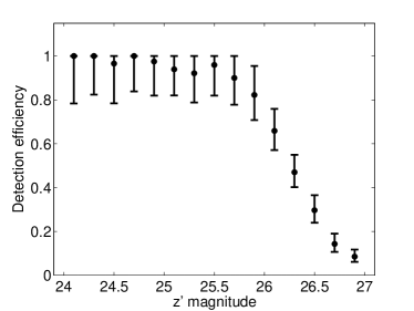
Figure 1: Fraction of simulated SNe recovered as a function of $z^{\prime}$-band magnitude. Error bars indicate $1\sigma$ Poisson uncertainties.

Each fake SN was assigned a random magnitude, but was kept in the sample only if it was no brighter than the magnitude a SN Ia would reach at peak at the given redshift of the host. We thus generated a list of positions and magnitudes for more than a thousand fake SNe. The objects were planted in the image using the IRAF task mkobject with a Gaussian profile. During the search, we could not distinguish between real and fake SNe. Our resulting efficiency as a function of magnitude can be seen in Figure 1. Our recovery rate is stable and nearly perfect, averaging 96%, up to $z^{\prime}=25$ mag, where it starts to decline. The efficiency is 50% at $z^{\prime}=26.3$ mag, and effectively reaches zero at $z^{\prime}=27$ mag. More than 80% of the 1000 simulated SNe are in the interesting magnitude range, between 25 and 27, where a good sampling of the efficiency curve is important. We have tested the effect of replacing the Gaussian profile of the fake SNe by an empirical profile measured from the image, using different template stars for different portions of the image, and found no changes in the efficiency compared to our previous simulations.

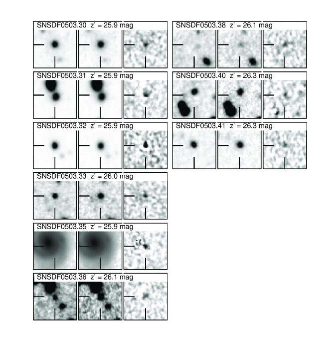
Figure 2: Image sections, $10^{\prime\prime}$ on a side, for the SNe in our sample. North is up, east is to the left. For each SN we show the reference and new epoch $z^{\prime}$-band images (left and centre, respectively), and the difference image (right). The greyscale for all the difference images is the same, while for the other images it is chosen to emphasize host-galaxy details.

3.3 Supernova Sample

We found a total of 33 SNe, shown in Figure 2, with magnitudes in the range $z^{\prime}=23.7$ to $z^{\prime}=26.3$. Table 1 lists the SNe and their properties. Our SNe do not have spectroscopic confirmation (indeed, spectroscopy for most of them is impossible with existing telescopes) or light curves, therefore they do not satisfy the International Astronomical Union criteria for a “standard” appellation. Nonetheless, since we are confident in our search and screening process (and also for the sake of brevity), we will refer to them as SNe, rather than SN candidates. We denote the SNe from this March 2005 run as “SNSDF$0503.$XX”, XX being a serial number, ordered roughly according to the SN $z^{\prime}$-band magnitude. The respective host galaxies are referred to as “hSDF$0503.$XX”. Ten of the 11 brightest SNe are also visible in the first image from KPNO. Apart from the 33 SNe, we detect several tens of candidates at fainter magnitudes, as we would expect based on our efficiency simulations (see 3.2), but these are 1$\sigma$ to 2$\sigma$ detections, which are mixed with an unknown number of false positives that arise from random peaks in the noise distribution and from subtraction artefacts. We therefore limit our sample to $z^{\prime}\leq 26.3$ mag, which leaves only candidates that we judge to be unambiguously real. Coincidentally, $z^{\prime}\leq 26.3$ mag is also our 50% detection efficiency limit.

ID	$\alpha$ (J2000)	$\delta$ (J2000)	$R$	$i^{\prime}$	$z^{\prime}$	S/Na	Photo-$z$	Spec-$z$	$P_{Ia}$b	Type	Posterior $z$	$\chi^{2}$	M${}^{c}0$
SNSDF0503.03	13:23:52.42	+27:12:45.36	24.58$\pm$0.08	23.98$\pm$0.08	23.71$\pm$0.08	35	0.91	0.886	0.98	Ia	0.89	0.95	$-19.3$ ($B$)
SNSDF0503.04	13:24:45.54	+27:18:14.06	24.08$\pm$0.08	24.04$\pm$0.08	23.83$\pm$0.08	33	0.43	$\cdots$	0.32	CC	0.34	0.08	$-17.3$ ($B$)
SNSDF0503.05	13:24:22.02	+27:16:06.99	24.70$\pm$0.08	24.25$\pm$0.08	23.85$\pm$0.08	56	0.59	0.593	0.90	Ia	0.59	1.19	$-17.8$ ($B$)
SNSDF0503.07	13:25:14.55	+27:29:16.46	25.26$\pm$0.08	24.52$\pm$0.08	24.12$\pm$0.08	37	0.91	0.918	0.95	Ia	0.92	0.93	$-19.0$ ($B$)
SNSDF0503.08	13:25:33.35	+27:36:39.61	25.10$\pm$0.08	24.51$\pm$0.08	24.26$\pm$0.08	46	0.69	0.707	0.78	Ia	0.71	0.20	$-18.0$ ($B$)
SNSDF0503.09	13:24:37.91	+27:36:38.00	25.64$\pm$0.09	24.99$\pm$0.08	24.55$\pm$0.09	27	0.67	$\cdots$	0.61	Ia	0.67	0.02	$-17.4$ ($B$)
SNSDF0503.10	13:25:28.58	+27:36:24.60	25.96$\pm$0.11	24.78$\pm$0.08	24.74$\pm$0.11	22	0.81	0.849	0.89	Ia	0.85	5.34	$-18.1$ ($B$)
SNSDF0503.11	13:25:06.01	+27:40:22.31	24.90$\pm$0.08	24.91$\pm$0.08	24.94$\pm$0.12	11	0.57	$\cdots$	0.50	Ia	0.57	2.32	$-17.2$ ($B$)
SNSDF0503.12	13:24:00.48	+27:26:04.13	27.08$\pm$0.31	25.40$\pm$0.10	24.93$\pm$0.12	17	0.73	$\cdots$	0.62	Ia	1.44	0.61	$-17.1$ ($U$)
SNSDF0503.13	13:23:54.85	+27:34:17.23	25.23$\pm$0.08	25.02$\pm$0.08	25.02$\pm$0.13	10	0.58	$\cdots$	0.17	CC	0.51	0.04	$-17.0$ ($B$)
SNSDF0503.14	13:24:09.34	+27:18:41.91	25.69$\pm$0.10	25.10$\pm$0.09	25.04$\pm$0.13	11	0.53	0.506	0.27	CC	0.51	0.39	$-16.3$ ($B$)
SNSDF0503.15	13:24:08.09	+27:35:21.78	$>27.10$d	26.05$\pm$0.17	25.08$\pm$0.14	13	$\cdots$	$\cdots$	0.71	Ia	1.27	0.00	$-19.4$ ($B$)
SNSDF0503.16	13:24:40.09	+27:18:34.25	25.97$\pm$0.12	25.52$\pm$0.11	25.18$\pm$0.15	13	1.15	$\cdots$	0.87	Ia	1.08	1.79	$-18.7$ ($B$)
SNSDF0503.17	13:25:06.12	+27:22:32.44	$>27.10$d	26.75$\pm$0.33	25.32$\pm$0.17	18	1.36	$\cdots$	0.88	Ia	1.36	1.07	$-19.5$ ($B$)
SNSDF0503.18	13:25:14.35	+27:28:52.83	$>27.10$d	26.02$\pm$0.17	25.31$\pm$0.17	9	$\cdots$	$\cdots$	0.57	Ia	1.60	0.47	$-18.4$ ($U$)
SNSDF0503.19	13:24:50.37	+27:45:16.61	$>27.10$d	26.46$\pm$0.25	25.44$\pm$0.19	8	1.89	$\cdots$	0.70	Ia	1.68	0.51	$-15.6$ ($U$)
SNSDF0503.20	13:24:57.75	+27:36:41.80	$>27.10$d	26.63$\pm$0.30	25.48$\pm$0.20	10	0.81	$\cdots$	0.80	Ia	0.88	0.06	$-16.8$ ($B$)
SNSDF0503.22	13:24:35.31	+27:19:41.64	25.75$\pm$0.10	25.42$\pm$0.10	25.43$\pm$0.19	7	0.43	0.450	0.17	CC	0.45	1.17	$-15.9$ ($B$)
SNSDF0503.23	13:24:48.19	+27:45:27.67	$>27.10$d	26.31$\pm$0.22	25.54$\pm$0.21	7	0.47	$\cdots$	0.25	CC	0.46	0.58	$-14.3$ ($B$)
SNSDF0503.24	13:24:21.80	+27:31:41.92	26.54$\pm$0.19	25.23$\pm$0.09	25.56$\pm$0.21	10	0.19	0.195	0.00	CC	0.20	22.17	$-13.2$ ($V$)
SNSDF0503.25	13:24:21.78	+27:13:22.77	$>27.10$d	26.28$\pm$0.21	25.63$\pm$0.22	9	0.51	0.530	0.36	CC	0.53	0.62	$-15.1$ ($B$)
SNSDF0503.26	13:24:21.51	+27:41:10.51	$>27.10$d	26.74$\pm$0.33	25.71$\pm$0.24	7	0.81	1.130	0.81	Ia	1.13	0.52	$-18.2$ ($B$)
SNSDF0503.27	13:25:24.24	+27:35:46.68	$>27.10$d	26.72$\pm$0.32	26.19$\pm$0.37	5	0.84	0.848	0.52	Ia	0.85	0.10	$-16.5$ ($B$)
SNSDF0503.29	13:24:42.38	+27:14:23.40	26.43$\pm$0.17	26.08$\pm$0.18	25.84$\pm$0.27	4	0.90	1.085	0.80	Ia	1.08	2.82	$-17.8$ ($B$)
SNSDF0503.30	13:24:12.86	+27:37:47.55	$>27.10$d	26.93$\pm$0.39	25.89$\pm$0.29	8	1.31	$\cdots$	0.72	Ia	1.30	0.52	$-18.7$ ($B$)
SNSDF0503.31	13:24:28.67	+27:44:47.68	26.29$\pm$0.15	26.01$\pm$0.17	25.88$\pm$0.28	6	0.96	1.080	0.68	Ia	1.08	4.87	$-17.7$ ($B$)
SNSDF0503.32	13:25:27.90	+27:33:06.09	$>27.10$d	$>27.00$d	25.88$\pm$0.28	7	1.05	1.214	0.82	Ia	1.21	1.03	$-18.6$ ($B$)
SNSDF0503.33	13:24:02.89	+27:17:53.77	26.57$\pm$0.19	26.70$\pm$0.32	26.03$\pm$0.32	7	1.22	$\cdots$	0.72	Ia	0.86	4.33	$-17.7$ ($B$)
SNSDF0503.35	13:24:22.24	+27:15:14.85	$>27.10$d	25.54$\pm$0.11	25.93$\pm$0.30	7	0.34	0.340	0.01	CC	0.34	30.07	$-13.2$ ($V$)
SNSDF0503.36	13:24:05.12	+27:38:45.62	26.75$\pm$0.23	26.34$\pm$0.23	26.14$\pm$0.36	7	0.87	$\cdots$	0.46	CC	0.87	0.26	$-16.8$ ($B$)
SNSDF0503.38	13:24:17.97	+27:15:43.49	$>27.10$d	$>27.00$d	26.12$\pm$0.35	5	1.87	$\cdots$	0.41	CC	0.30	0.43	$-17.0$ ($V$)
SNSDF0503.40	13:23:39.00	+27:21:03.11	$>27.10$d	$>27.00$d	26.34$\pm$0.43	3	1.83	1.564	0.95	Ia	1.56	0.96	$-15.1$ ($U$)
SNSDF0503.41	13:25:22.36	+27:41:02.41	$>27.10$d	26.43$\pm$0.25	26.34$\pm$0.42	4	0.70	0.709	0.32	CC	0.71	1.51	$-15.9$ ($B$)

Table 1: Supernovae Discovered in the Subaru Deep Field. ^a Signal-to-noise ratio of the SN, in the $z^{\prime}$-band image. ^b Probability that object is a SN Ia, based on SN-ABC (P07). ^c Approximate absolute magnitudes in rest-frame $B$ band, unless rest-frame $B$ does not fall within the observed $R,i^{\prime},z^{\prime}$ bands, in which case we list rest-frame $U$ or $V$ absolute magnitudes, at high or low redshift, respectively. ^d Fainter than $3\sigma$ limiting magnitude in this band.

Aperture photometry of the SNe was performed on the difference $R$, $i^{\prime}$, and $z^{\prime}$ images, using SExtractor, and adopting a $2\arcsec$ diameter circular aperture. To estimate the photometric uncertainty, we measured the magnitudes of the $1000$ simulated transients planted in the image for the efficiency measurements (see §3.2), and took the root mean square (rms) in each magnitude bin to be the minimum photometric error for objects of that magnitude. The adopted uncertainty for each SN was taken to be the larger among the formal error computed by SExtractor and the statistical error for the given magnitude from the simulated objects. For each SN we derived the local S/N by comparing the SN counts in the photometric aperture, to the standard deviation of the total counts in tens of identical apertures on nearby, similar, background. We also measure the offset between the simulated SN positions as input to the images, and as found by SExtractor. All the simulated SNe are found within $0\aas@@fstack{\prime\prime}10$ of their intended positions, and 93% are within $0\aas@@fstack{\prime\prime}04$. We use these results to estimate the accuracy to which an offset between a SN and its host-galaxy centre can be detected.

The two SNe closest to their respective host centres have measured offset of $0\aas@@fstack{\prime\prime}07$ and $0\aas@@fstack{\prime\prime}08$, while all others have offsets greater than $0\aas@@fstack{\prime\prime}10$, effectively ruling out an AGN classification for most, if not all, objects.

4 Supernova Host Galaxies

In this section, we determine which galaxy hosts every SN, and measure its properties. This allows us to measure the redshift of the SNe, and eventually, will permit a study of the correlations between the properties of SNe and their host galaxies.

4.1 Identification and Photometry

For our list of SNe, we compiled a list of potential host galaxies. We measured the Petrosian magnitudes (Petrosian 1976) of the host galaxies on the reference (deeper) epoch, in seven bands, with SExtractor. Petrosian magnitudes allow one to measure the flux of resolved objects within a given fraction of the light profile, without the dependence on the amplitude of the surface brightness profile associated with “isophotal” magnitudes (e.g., Blanton et al. 2001; Graham et al. 2005). As for the SN photometry, we estimated the uncertainty in each magnitude bin using artificial sources with galactic profiles that we planted in the images.

The hosts of the SNe were chosen based on the smallest separations between each SN and its neighboring galaxies, in terms of each of the galaxies’ half-light radii, as measured with SExtractor in the $i^{\prime}$ band. For most of the SNe, the choice was obvious, since the SNe and their hosts were unresolved from each other.

For two SNe (SNSDF$0503.15$ and SNSDF$0503.18$) we found no plausible host within 6 half-light radii. Assuming a Sersic (1968) model for the galaxy radial profile between $n=4$ (de Vaucouleurs law; de Vaucouleurs 1948; Peng et al. 2002) and $n=1$ (exponential disk; Freeman 1970; Peng et al. 2002), we find that between 91% and 99.99% of the light, respectively, is within 6 half-light radii . The probability that a SN belongs to a host at a distance beyond this limit is thus small. Due to the high density of sources in the SDF, using a larger limit would lead to confusion regarding the hosts of most of the SNe, including those SNe which are unresolved from a particular galaxy. The two SNe which we label as “hostless” are probably the result of a host that is below our detection threshold in all the photometric bands (though these SNe could, in fact, be hostless; see Gal-Yam et al. 2003). Alternative explanations are that these candidates are actually flaring Galactic M-dwarfs or variable AGNs in faint hosts. The non-detection of a source at this position in the reference epoch, down to $i^{\prime}\approx 27.5$ mag, means that a star with a quiescent absolute magnitude of $M_{i}\approx 8$ (e.g., Thé, Steenman & Alcaino 1984) would be at a distance $>80$ kpc, making this option highly improbable. The possibility of a high-$z$ AGN cannot be excluded. Nevertheless, the $\chi^{2}$ criterion we apply to the candidates (see §5) does not support this interpretation. Table 2 lists the SN hosts and their properties.

Table 2: SN Host Galaxies. ^a Arcseconds. ^b Best-fitting galaxy template. SB2 is a starburst spectral template from Kinney et al. (1996). ^c Fainter than $3\sigma$ limiting magnitude in this band.

4.2 Host Redshifts

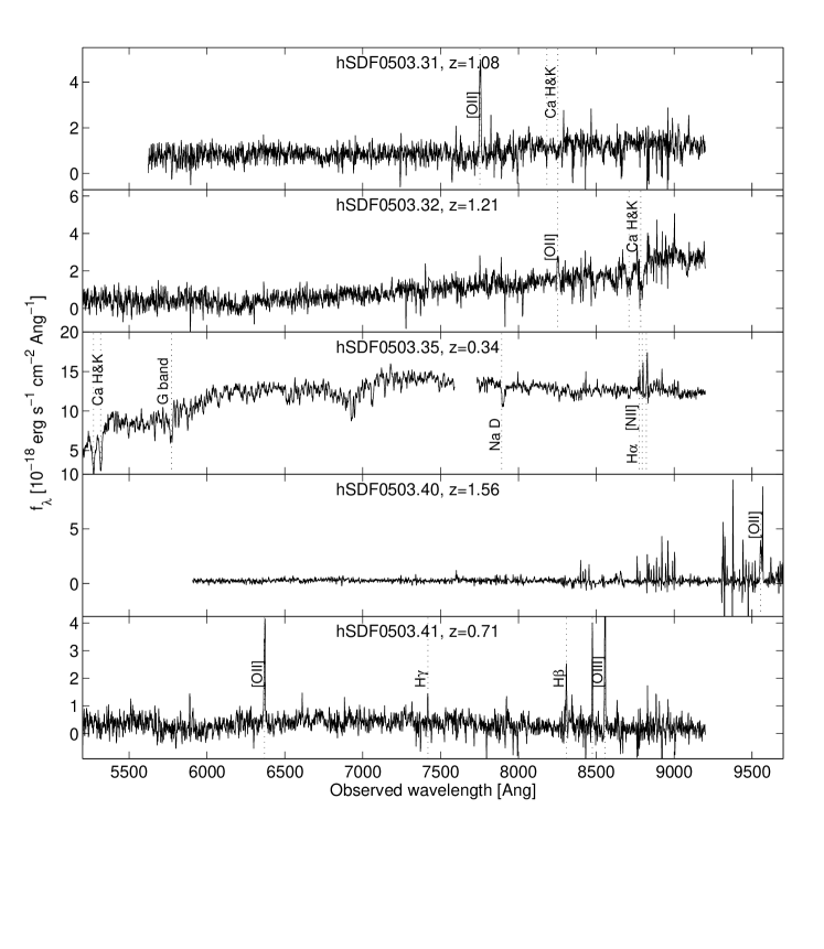
Figure 3: Keck DEIMOS spectra for 17 of the SN host galaxies. For most galaxies, the redshift is securely determined by several emission or absorption lines. In hSDF$0503.03$, hSDF$0503.26$, and hSDF$0503.40$, the single line is double peaked, making the identification as [O ii] $\lambda\lambda$3726, 3729 quite robust. Regardless, any other assignment predicts the presence of other lines which we do not detect. Gaps in the spectra correspond to regions with strong night-sky line subtraction residuals.

We find the redshifts of the host galaxies using a combination of photometry and spectroscopy. Out of 19 host galaxies with $R<25~{}\mathrm{mag}$, the approximate practical limit for spectroscopy, we observed 18, and managed to measure 16 redshifts. We also measured redshifts for a fainter host, hSDF$0503.03$, with $R=25.8$ mag. The spectra are shown in Figure 3. The spectra of hSDF$0503.16$ and hSDF$0503.17$, which were presumably bright enough for Keck ($R=23.56$ mag and $R=24.91$ mag, respectively), did not yield a conclusive redshift, probably due to slit imperfections that impair proper sky-line subtraction. We note that no spectrum shows an AGN signature (except hSDF$0503.35$ that hosts a LINER offset from the SN, see §5).

The highest spectroscopic redshift we obtained is $z=1.564$, for hSDF$0503.40$, slightly higher than the redshift of the host of SN 2003ak found by GOODS at $z=1.551$ (Riess et al. 2004a). This makes SNSDF$0503.40$ the SN with the highest host spectroscopic redshift reported to date. SN 1997ff at $z\approx 1.7$, like other SNe in our sample having comparable photometric redshifts, does not have a spectroscopic SN or host redshift (Riess et al. 2001).

In order to assemble a training set for the derivation of photo-$z$, we measured 145 spectroscopic redshifts (123 of which are secure) for galaxies chosen randomly near the positions of the SN hosts, at first with no selection criteria other than sufficient brightness for spectroscopy ($i^{\prime}<25~{}\rm{mag}$). In the last Keck run, we preferentially selected galaxies with photometric redshifts between 1.5 and 2, in order to better sample that region of parameter space. The redshifts for these 123 galaxies are listed in Table 3 in the online version of this paper. We supplement these data with spectroscopic redshifts for a sample of SDF galaxies that were obtained for other SDF-related projects (e.g., Kashikawa et al. 2003, 2006; Shimasaku et al. 2006), usually selected for their excess flux in the narrow-band filters $NB816$ and $NB921$ (designed to detect Ly$\alpha$ emission lines at redshifts near 5.7 and 6.6, respectively). From this sample we select 196 galaxies with secure $z<2$ redshifts. This results in a set of 319 galaxies with secure redshifts that allows us to tune and test the photo-$z$ determination. While this sample is quite extensive, it is probably biased toward galaxies with bright emission lines, for which spectroscopic redshifts are easier to measure.

ID	$\alpha$ (J2000)	$\delta$ (J2000)	$R$ mag	Redshift	Instrumenta
1	13:23:51.556	+27:11:51.53	24.3	1.488	4
2	13:23:40.027	+27:13:01.35	23.7	0.287	4
3	13:24:37.571	+27:13:24.44	23.4	0.736	2
4	13:24:21.800	+27:13:22.62	23.1	0.530	2
5	13:24:30.644	+27:13:37.35	25.1	1.466	2
$\cdots$
$\cdots$

Table 3: Keck Spectroscopy of SDF Galaxies. The full table is available in the electronic version of the paper. ^a Instrument and observation date: 1 = LRIS, 12 Jan. 2007; 2 = DEIMOS, 21 Jan. 2007; 3 = DEIMOS, 16 Mar. 2007; 4 = DEIMOS, 12 Apr. 2007.

For the derivation of the SN host photometric redshifts, we have used the recent version of the Zurich Extragalactic Bayesian Redshift Estimator (ZEBRA; Feldmann et al. 2006). Briefly, ZEBRA works as follows. First, the photometry catalog is corrected for systematic errors by finding residuals in a first fit to a set of basic galaxy spectral templates. Next, the templates are corrected using a training set with spectroscopic redshifts. Finally, the redshifts are derived using a Bayesian methodology, where the redshift and best-fitting template for each galaxy are found iteratively, while using the resulting distributions (both in redshift and template space) as priors. Our initial templates are the same ones used by Benítez (2000). For the correction of the photometry, we measured all the objects in the SDF, following the procedure described in §3.3 for the photometry of the SN host galaxies. The six basic templates that are used in BPZ (for galaxy types elliptical, Sbc, Scd, irregular, and two types of starburst) were interpolated to produce three intermediate galaxy types between every two consecutive templates. The resulting 21 templates were then corrected using a partial (early) version of the training set described above, of about 200 galaxies. The correction was done in three redshift bins ($z<0.5$, $0.5<z<0.9$, $z>0.9$). This resulted in 84 templates (the 21 original interpolated ones plus 21 for each redshift bin). The resulting posterior redshift distribution of all the galaxies in the SDF was used as a prior for the SN host redshifts. We set the limit on the absolute rest-frame $B$-band magnitude of the galaxy to lie, conservatively, between $-26$ and $-10$.

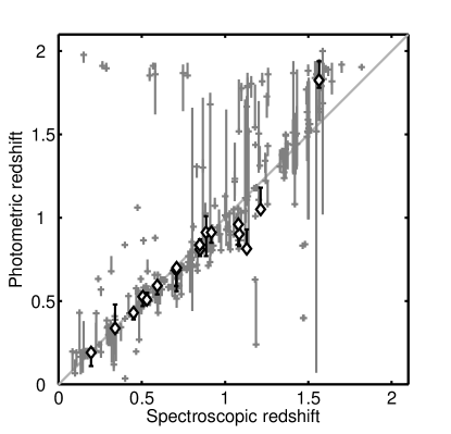
Figure 4: Comparison of the spectroscopic redshifts and the ZEBRA photometric redshifts for the random sample of 319 galaxies (grey crosses), and for 17 SN host galaxies (empty diamonds). Error bars indicate the 68.3% confidence interval of the $z$-pdf for each galaxy. The scatter of the random sample with photo-$z$ smaller than $1.8$ is $\sigma_{z}/(1+z)=0.08$ after excluding five $4\sigma$ outliers. For the SN host sample the scatter is $\sigma_{z}/(1+z)=0.06$.

Figure 4 shows the results of using ZEBRA on our training set. First, one can see that the photo-$z$ determination is usually in good agreement with the spectroscopic redshift. On the other hand, photo-$z$ values above 1.8 are many times unreliable for this training-set sample. Restricting ourselves to photometric redshifts smaller than $1.8$, where 93% of our sample is located (and probably all of our SNe), leaves us with 296 galaxies, with a dispersion of $\sigma_{z}/(1+z)=0.08$ after rejecting five $4\sigma$ outliers (less than 2% of this sample). The scatter for our sample of 17 SN host galaxies is somewhat smaller, $\sigma_{z}/(1+z)=0.06$, without a single outlier rejected. Application of the Kolmogorov–Smirnov test to the two samples of residuals indicates that the difference is not significant.

Improvement to the photo-$z$ derivation could come from an extension of the imaging data to the near-infrared, as the rest-frame 4000–8000 Å range is shifted, at $z\approx 1.8$, into the $J$, $H$, and $K$ bands. With existing wide-field near-IR imagers (e.g., WFCAM on the UKIRT, Casali et al. 2001), and certainly future ones (e.g., NEWFIRM on the NOAO telescopes, Autry et al. 2003), deep imaging in those bands of well-studied fields, such as the SDF, would be extremely useful for projects such as ours.

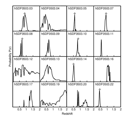
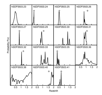
Figure 5: Redshift probability density functions ($z$-pdfs) of the SN host galaxies, as calculated with ZEBRA, and used as priors for the SN classification. Grey crosses mark the spectroscopic redshifts, when available. Notice the complex shapes of the $z$-pdfs, and the agreement in most cases between the most probable photo-$z$ and the spectroscopic redshift. All $z$-pdfs have a total probability of 1; the vertical scale varies from frame to frame.

The output from ZEBRA that we use is the redshift probability distribution function ($z$-pdf) for each host galaxy, which is obtained by marginalizing the full posterior distribution over all templates. The resulting $z$-pdfs of our host sample are shown in Figure 5. The $z$-pdf can have a complex structure — it is not necessarily a single peaked, well-behaved, function. For example, the distribution for hSDF$0503.03$ is clearly bimodal, while that of hSDF$0503.12$ contains very little information, with all redshifts almost equally likely. Using the full $z$-pdfs in the subsequent analysis allows us to take this uncertainty into account. Out of the 31 host $z$-pdfs, 23 have widths $w_{z}/(1+z)<0.08$, where $w_{z}$ is the standard deviation of the best-fitting Gaussian to the $z$-pdf, while only three have $w_{z}/(1+z)>0.2$ (namely hSDF$0503.12$, hSDF$0503.19$, and hSDF$0503.38$). For 16 of the 17 host galaxies for which we have a spectral redshift, it is very close (usually nearly identical) to the photo-$z$, with $\Delta z/(1+z)\leq 0.1$, while for the remaining galaxy (hSDF$0503.26$) it differs by only $\Delta z/(1+z)=0.15$. For these 17 galaxies, we use in the subsequent analysis a Gaussian $z$-pdf centered on the measured spectroscopic redshift, with a width $w_{z}=0.01$. For the two hostless SNe (SNSDF$0503.15$ and SNSDF$0503.18$), we use a flat redshift prior between 0 and 2. Table 2 lists the measured properties of the SN host galaxies, including the best-fitting redshifts and template types.

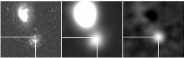
Figure 6: Left: image section of $HST$-ACS image of the host galaxy of SNSDF$0503.31$. Centre: $R$-band SuprimeCam image prior to SN explosion. Right: difference between SuprimeCam images. There is a clear offset between the SN and its host centre, a face-on spiral galaxy.

The region of the SN host galaxy hSDF$0503.31$ was imaged with HST/ACS. As seen in Figure 6, this host is a face-on spiral galaxy, consistent with the photo-$z$ best-fitting template, with the SN clearly offset from the centre by $0\aas@@fstack{\prime\prime}35$. While this $z=1.08$ galaxy seems to be associated with the brighter spiral seen in the figure, the photo-$z$ of the bright galaxy is much smaller, $z\approx 0.5$.

5 Supernova Classification

The next step in our analysis is the classification of the SNe into types, based solely on our single-epoch photometry and the redshift information for the hosts. P07 have recently developed for this purpose an algorithm, the SN Automatic Bayesian Classifier (SN-ABC). Briefly, the SN-ABC is a template-fitting routine that compares the SN magnitudes to synthetic magnitudes derived from a library of template SN spectra of different types, ages, redshifts, and extinctions. The input to SN-ABC is the photometry of the SN and the $z$-pdf of its host, which is used as a redshift prior. The output is the probability that the SN is of Type Ia, $P_{Ia}$, compared to the probability it is a core-collapse event, $P_{CC}=1-P_{Ia}$, a posterior $z$-pdf, and a $\chi^{2}$ value. The $\chi^{2}$ criterion permits rejecting candidates with colours unlike those of SNe, usually peculiar SNe, AGNs, or other transients or variables, that were not rejected in previous steps based on their variability characteristics. As shown in P07, more than half of the AGNs can be rejected in this manner. A SN with value of $P_{Ia}>0.5$ is considered to be of Type Ia, while objects with $P_{Ia}<0.5$ are classified as CC-SNe. As shown in P07, $P_{Ia}$ also serves as a confidence estimator. The closer it is to unity (zero), the more secure is the classification as a SN Ia (CC-SN).

P07 tested the algorithm on different real and simulated datasets. The SN-ABC successfully classifies 97% of the SNe Ia from the Supernova Legacy Survey (SNLS; Astier et al. 2006), and 85% of the Type II-P SNe. Similar success fractions were obtained for the GOODS SNe, and for a simulated sample. These simulations also show that for Type Ib/c SNe, success fractions are smaller (about 75%), while Type IIn SNe are often misclassified as SNe Ia. The resulting purity of a SN sample depends on the details of the survey. Consequently, in §6 we perform simulations with parameters tailored to our survey, and use them to “debias” our sample, and to determine the range of type distributions consistent with the data.

Table 1 lists the SNe we have found, their redshifts, and their ABC classifications. Among the 33 SNe, 22 are classified as SNe Ia by the algorithm. Among these 22 SN Ia classifications, 16 have $P_{Ia}$ values higher than 0.7, while 6 of the 11 CC-SNe are classified with similar confidence, $P_{CC}>0.7$.

Two SNe, SNSDF$0503.24$ and SNSDF$0503.35$, have extreme $\chi^{2}$ values of 22.2 and 30.1, respectively. As discussed above, this could be indicative of a non-SN object, since, as shown in P07, the SN-ABC assigns high $\chi^{2}$ values to most AGNs. However, both are well offset from the centres of their host galaxies. The host hSDF$0503.35$ is a “grand-design” face-on spiral galaxy (Fig. 2) having a LINER spectrum (Ho, Filippenko & Sargent 1997) with an H$\alpha$ luminosity of $\sim 10^{39}$ erg s^-1, typical of such objects. Thus, these are probably not AGNs (see, however, Gal-Yam 2005 and Gal-Yam et al. 2007, in preparation, who found a background AGN projected near a lower-redshift galaxy). Both of their respective hosts have relatively low (spectroscopic) redshifts, and are, in fact, the lowest-redshift SNe in our sample. Both are classified as CC-SNe, with high confidence, which in the context of the SN-ABC means that their colours resemble significantly more those of a SN II-P than a SN Ia. However, the large $\chi^{2}$ values imply that neither SN type is a good fit. Since these are unlikely to be SNe Ia, we keep them in our CC-SN sample. Nevertheless, we will continue to monitor these positions in future observations, in order to test the background AGN option.

We also note that hSDF$0503.35$ is classified by ZEBRA as an elliptical galaxy, in contradiction with its spiral morphology. This is probably due to the photometry being dominated by the bulge, while the SN could be in the disc. Another CC-SN host, hSDF$0503.23$, is also classified as an elliptical, suggesting that, here as well, the classification, either of the host galaxy, or of its SN, is erroneous. However, we expect a fraction of the SNe to be misclassified, and we deal explicitly with the resulting uncertainties and biases in §6.

The posterior redshift, derived from the combined fit of each SN and its host, is generally quite close to the prior (host-galaxy-only based) redshift, but as shown in P07, these posterior redshifts can sometimes be biased, and therefore we generally do not use them in the next step. A clear example of disagreement between a prior and a posterior redshift is SNSDF$0503.38$, which has a prior redshift of 1.87, while the SN photometry combined with this prior yields a classification as a CC-SN at $z=0.3$. This apparent discrepancy is easily understood if one notices that the $z$-pdf for the host galaxy of this SN is very wide and unconstraining, and hence the best-fitting redshift for the host is quite meaningless. For this object, as well as for SNSDF$0503.12$ and SNSDF$0503.19$ that have similarly wide $z$-pdfs, and the hostless SNSDF$0503.15$ and SNSDF$0503.18$, we use the posterior redshifts that take into account the SN properties.

For a rough idea of the properties of the SNe, we use the peaks of the $z$-pdfs as best-fitting redshifts, and find approximate rest-frame absolute magnitudes of the SNe. First, we fit the de-redshifted fluxes with a linear function, to describe the spectral energy distribution (SED) of the SN. We then perform synthetic photometry in the $B$ band, unless rest-frame $B$ does not fall within the observed $R$, $i^{\prime}$, or $z^{\prime}$ bands. In such a case, we derive rest-frame $U$ or $V$ absolute magnitudes, at high or low redshift, respectively. The resulting absolute magnitudes, listed in Table 1, range between $-13.2$ and $-17.3$ for the CC-SNe, and between $-15.1$ and $-19.5$ for the SNe Ia.

We divide the samples of SNe Ia and CC-SNe into four redshift bins ($z<0.5$, $0.5<z<1.0$, $1.0<z<1.5$, and $1.5<z<2.0$), using the peak of the $z$-pdfs as best-fitting redshifts. These “raw” distributions are shown in Fig. 7 and listed in Table 4.

6 Uncertainties, Sample Contamination, and Derivation of Intrinsic Supernova Type and Redshift Distributions

The ABC classification can introduce biases due to the dependence of the success fraction on the intrinsic parameters (type, age, redshift) of the SNe. We therefore use Monte Carlo simulations to determine the allowed range, and the most likely “true” redshift and type distribution, of the SNe (as we would have observed if we had perfect spectroscopic data for all of the SNe and their hosts).

Following P07, we have randomly generated $10,000$ SN spectra of each of the main SN types: Ia, Ibc, II-P, and IIn (see, e.g., Filippenko 1997). We calculate the synthetic magnitudes of the fake SNe using the SEDs from the spectral templates of Nugent, Kim & Perlmutter (2002) for SNe Ia, Ib/c, and II-P. Since the Nugent et al. (2002) spectra of SNe IIn are theoretical blackbody SEDs, for this type only we use the templates from Poznanski et al. (2002). Absolute magnitudes and their dispersions are taken from Dahlen et al. (2004). The scatter in colour within each type is applied to the CC-SNe by adding an intrinsic, normally distributed, noise with a standard deviation of $\sigma=0.2~{}\mathrm{mag}$, the value used by Sullivan et al. (2006a). The SNe Ia we simulate are assigned different stretch values $s$, following the method described by Sullivan et al. (2006a). We simulate a Gaussian distribution of stretch values with an average of $s=1$ and a dispersion of $\sigma=0.25$, truncated outside the range $0.6\leq s\leq 1.4$. We model the stretch-luminosity relation using the formalism $M_{Bc}=M_{B}-\alpha(s-1)$ (Perlmutter et al. 1999), where $M_{Bc}$ and $M_{B}$ are the corrected and uncorrected $B$-band absolute magnitudes, respectively, and the correlation factor is $\alpha=1.47$. We also apply colour-stretch corrections using the method presented by Knop et al. (2003), by dividing the template spectra of normal, $s=1$, SNe Ia, by smooth spline functions, in order to match their rest-frame $UBVRI$ colours to those of SNe with various stretch values.

To every simulated SN we assign an epoch, a host-galaxy extinction, and a redshift. The epoch is drawn from a uniform distribution, while the host extinction, $A_{V}$, is drawn from the positive side of a Gaussian distribution with maximum at zero, $\sigma=0.2$ mag for SNe Ia, and $\sigma=0.5$ mag for CC-SNe, truncated at $A_{V}=1$ mag. The redshifts are drawn from the general galaxy population in the SDF using the following scheme. A realistic photometric redshift is modeled, by drawing, for half of the SNe, the $z$-pdf of a random SDF galaxy with $z<2$. To the other half of the simulated SNe we assign a spectroscopic redshift, by using a $\sigma=0.01$ Gaussian $z$-pdf. This mimics the redshift determination characteristics of the real sample. We have measured the widths of the simulated sample’s $z$-pdfs, as well as of the real host-galaxy sample, by fitting them with Gaussians, and find that the simulated and real samples have similar distributions of widths. We draw a specific redshift for each simulated SN from its $z$-pdf, and use it to redshift the simulated spectrum.

We then fold the simulated SN spectra through the observational setup of our SDF observations, with their three bandpasses, photometric errors, and limiting magnitudes. We have measured the mean photometric errors of the SDF sample in each band as a function of magnitude, and assuming that the noise is normally distributed, have added it to each object. As with the real sample, we keep only objects with $z^{\prime}$-band magnitudes brighter than $26.3$, leaving $4,000$ of each type. The simulated SNe are then blindly classified by the ABC into SNe Ia or CC-SNe, producing a mapping of success fraction vs. redshift for each SN type. We find the success fractions of the ABC in four redshift bins ($z<0.5$, $0.5<z<1.0$, $1.0<z<1.5$, and $1.5<z<2.0$) for each of the four SN types.

The success fractions are applied to the set of all possible intrinsic type distributions (e.g., 30% SN Ia, 30% SN II-P, 20% SN Ib/c, and 10% SN IIn). Using steps of 2.5%, there are $12,341$ possibilities to distribute 100% of the observed SNe, in each redshift bin, among the four types. We compute, for each of these possibilities, the resulting fraction of objects that are labelled as SNe Ia in the sample (i.e., the sum of the fraction of SNe Ia that were correctly classified), and of the fraction of CC-SNe that were misclassified as SNe Ia, as obtained by the average success fractions for each type of SN, in each redshift bin. Next, for each scenario, in each redshift bin, we find the binomial probability to draw the observed raw number of SNe Ia out of the total number of SNe in the bin, given the expected SN Ia fraction for that scenario. Since, in this scheme, the SN Ia fractions do not have equal prior probability (e.g., there is only one model with 100% SNe Ia, while there are many with 50% SNe Ia and various fractions for the CC-SN subtypes), we multiply each probability by a weight function that is inversely proportional to the number of scenarios with the same SN Ia fraction. Finally, we marginalize over all the scenarios in each redshift bin, and obtain the probability density function for the true SN Ia fraction in that bin. From the probability distribution function of the SN Ia fraction in each bin, we extract the most probable value, at the peak of the distribution, and the $1\sigma$ uncertainties defined as the region that includes $68.3\%$ of the probability density. We add to this error the corresponding fraction of the $1\sigma$ Poisson uncertainty in that bin — that is, the Poisson uncertainty for the total number of SNe in the bin multiplied by the relevant fraction of SNe Ia. The most probable SN Ia fraction comes out the same as the SN Ia fraction given by the SN-ABC in two out of the four redshift bins. Only in the second redshift bin, $0.5<z<1.0$, is the debiased most-probable fraction of SNe Ia reduced from 0.64 to 0.39. The raw and debiased redshift distributions of the SNe Ia and CC-SNe are listed in Table 4, and shown in Figure 7. We discuss the results in the following section.

Sub-sample	$z<0.5$	$0.5<z<1.0$	$1.0<z<1.5$	$1.5<z<2.0$
SN Ia - (raw)	0	9	10	3
SN Ia - de-biaseda	$0.0^{+1.7+0.0}_{-0.0-0.0}$	$5.5^{+4.2+1.9}_{-3.8-1.4}$	$10.0^{+0.0+4.3}_{-4.4-3.1}$	$3.0^{+0.0+2.9}_{-1.5-1.6}$
CC-SN - (raw)	6	5	0	0
CC-SN - de-biaseda	$6.0^{+0.0+3.6}_{-1.7-2.4}$	$8.5^{+3.8+2.9}_{-4.2-2.3}$	$0.0^{+4.4+0.0}_{-0.0-0.0}$	$0.0^{+1.5+0.0}_{-0.0-0.0}$
Total	6	14	10	3
SN Ia rateb [10-5 Mpc${}^{-3}\,$yr-1]	$0.0^{+2.4}_{-0.0}$	$4.3^{+3.6}_{-3.2}$	$10.5^{+4.5}_{-5.6}$	$8.1^{+7.9}_{-6.0}$

Table 4: Supernova Redshift Distribution. ^aErrors are $1\sigma$ classification and Poisson uncertainties, respectively. ^b SN Ia rate errors are classification and Poisson uncertainties added in quadrature

Figure 7: Observed, raw (circles; slightly offset to the right for clarity), and debiased (lines), redshift distributions of SDF SNe Ia and CC-SNe, compared to the GOODS sample (squares; offset to the left). SDF error bars mark $1\sigma$ classification and Poisson errors, added in quadrature. GOODS error bars denote $1\sigma$ Poisson uncertainties. The debiased SDF and GOODS distributions are consistent to within the uncertainties, but there is a suggestion of more high-$z$ SNe Ia in the SDF.

7 Comparison to the GOODS Supernova Sample

Before calculating rates, which requires some assumptions and modeling of the SN properties, we compare our SN sample to the most similar one in terms of depth and numbers, the GOODS SN sample. As part of the GOODS project, two fields of about $150~{}\textrm{arcmin}^{2}$ each were observed with the ACS camera on HST every 45 days, over five epochs, in order to search for SNe. We have compiled from Riess et al. (2004a) and Strolger et al. (2004) all available photometry for the 42 SNe found in the GOODS fields. These SNe cover a redshift range of $0.2$ to $1.55$, with a median of $0.76$. The SNe have partial light-curve coverage, and not all have spectroscopic redshifts or types. However, GOODS is a complete sample, without any subsequent selection.

Our survey and GOODS have different effective areas and observing strategies, for which we need to account prior to comparison. In terms of bands, the surveys are similar. The filter-plus-system bandpasses of the Suprime-Cam $z^{\prime}$ filter and of the HST F850LP filter (used by GOODS) have effective wavelengths at $9067\,$Å and $9082\,$Å, respectively. The GOODS detection efficiency function, as described by Strolger et al. (2004), is slightly deeper than our own, by about 0.1–0.2 mag. We consider only SNe brighter than our 50% efficiency limit, $z^{\prime}=26.3$ mag. For $z^{\prime}$-band magnitudes brighter than 26.3, both surveys have similar efficiencies, and no correction is needed for a comparison to be made, if we exclude the fainter GOODS SNe. The SDF covers $\sim 900~{}\mathrm{arcmin}^{2}$, and has a single epoch, since we searched for SNe only in the March 2005 images. GOODS covered $300~{}\mathrm{arcmin}^{2}$, imaged at five epochs, each separated by about 45 days, i.e., 2–4 weeks in the typical SN rest frames. This means that the epochs are not independent and cannot be simply summed, since most SNe are discovered early and are detected in more than one epoch. From the photometry in Riess et al. (2004a) and Strolger et al. (2004), we find that, out of 42 SNe, 38 are detected (i.e., brighter than 26.3 mag, our SDF cutoff magnitude) in $1.45$ epochs, on average, while the remaining 4 are too faint. Thus, the effective GOODS area is roughly $5\times 300~{}\mathrm{arcmin}^{2}/1.45=1036~{}\mathrm{arcmin}^{2}$, about 15% more than the SDF. Hence, for a direct comparison of the two samples, the number of GOODS SNe needs to be trimmed down from 38 to $38/1.15=33$. Due to this reduction factor, we will present non-integer numbers of SNe from GOODS in the discussion below.

Thus, after the normalization for the different effective areas, there are (coincidentally) exactly the same number of SNe in our sample and in the “SDF-normalized” GOODS sample (33), 18.9 of which are SNe Ia (compared to the most probable value of 18.5 in the SDF debiased sample) and 14.1 CC-SNe (most probable value 14.5 in the SDF). In Figure 7, we compare the redshift distributions for the SN Ia and CC-SN subsamples from the two surveys. Since one of the CC-SNe in the GOODS sample (SN 2002fv) has no redshift information, we exclude it from this comparison. As can be seen, the two samples agree well in total size, in total type fractions, and in the CC-SN redshift distribution.

However, the redshift distributions may differ for the SNe Ia. Our lowest-redshift SN Ia is at $z\approx 0.5$, while GOODS found SNe Ia down to $z\approx 0.2$. Furthermore, the SNe Ia in our sample reach higher redshifts, up to $z\approx 1.6$, rather than $z\approx 1.4$, in the “SDF-normalized” GOODS sample. While formally the distributions are consistent, our data could indicate that the results in Strolger et al. (2004) and Dahlen et al. (2004) concerning the paucity of SNe Ia at high $z$, and the implications for the SN Ia delay time, may change once larger samples are obtained. On the other hand, one of our high-$z$ SNe Ia, SNSDF$0503.18$, at $z=1.60$, is hostless, and its redshift is based solely on the posterior fit from the SN-ABC to the SN photometry. If this redshift is in error, the number of SNe Ia in the highest-redshift bin would be more similar to that of GOODS. At $z=0.55$, where the fraction of SNe Ia in our sample was most significantly reduced by the debiasing of our photometrically classified sample, lies the largest disagreement between competing measures of the SN Ia rates. Barris & Tonry (2006), who used photometric methods to classify SNe, found a rate 4–5 times higher than measured by Pain et al. (2002) and Neill et al. (2006). Neill et al. (2006) have suggested that the sample of Barris & Tonry (2006) may have suffered from contamination by CC-SNe. Our raw sample of SNe Ia in that same bin, without debiasing, would certainly be contaminated by CC-SNe.

8 The Type Ia Supernova Rate

The SN redshift distributions that we have derived can be used to set constraints on the SFH and SN Ia delay functions. However, our SN sample is still small, and considering the similarity in the redshift distributions of the SDF and GOODS CC-SN samples, we postpone a CC-SN rate derivation to future papers. Nevertheless, we calculate SN Ia rates, to examine how the differences in the distributions noted in §7 propagate into the underlying rates. We calculate the volumetric rate of SNe Ia, in four bins,

$$r_{Ia,i}=\frac{N_{Ia,i}}{\int{\eta(z)\,dV}},$$

where $N_{Ia,i}$ is the number of SNe Ia in bin $i$, and $\eta(z)$ and $dV$ are, respectively, the survey control time (see below) and the co-moving volume element (in Mpc^-3), as a function of redshift $z$. The integration is done within the limits of each bin. The control time, $\eta(z)$, is found as follows. For every redshift $z$, we calculate the model $z^{\prime}$-band SN Ia light curve, $m_{z}(t)$, and sum over the survey efficiency, $\epsilon(m)$, at these magnitudes:

$$\eta(z)=\int{\epsilon(m_{z}(t))\,\frac{dm}{dt}\,dt}.$$

The effective redshift of each bin, $<z>_{i}$, is defined as

$$<z>_{i}=\frac{\int{\eta(z)\,z\,dV}}{\int{\eta(z)\,dV}},$$

i.e., a mean redshift weighted by the volume and the control time.

The uncertainties are the Poisson and classification uncertainties of the sample, added in quadrature. To investigate how errors in the efficiency function plotted in Fig. 1 might propagate to our rate measurement, we have fitted the efficiency curve with a Fermi-Dirac-like step-function, derived the uncertainties in its parameters, and have repeated the rate calculation hundreds of times with randomly drawn efficiency curves. The resulting $1\sigma$ dispersion in the SN rates is of the order of $10^{-6}$Mpc^-3yr^-1, i.e., about 30 times smaller than the main sources of uncertainty. If, for some unknown reason, our detection efficiency curve is offset by $0.1$ mag, the derived rates would change by about 15%, again less than the main sources of uncertainty. A significantly larger shift of the efficiency function,e.g., by 0.3 mag toward bright magnitudes, would lower the efficiency to near zero at $z^{\prime}=26.3$ mag, and would be inconsistent with our having discovered SNe in this magnitude range (unless, of course, the intrinsic number of SNe rises sharply precisely at this brightness). We further neglect dust extinction in this rough derivation of the rate. As found by Riello & Patat (2005) and Neill et al. (2006), such an omission causes the rates to be underestimated by $\sim$25% at most, which is smaller than the uncertainties already taken into account. We also do not attempt at this point to incorporate SNe with different stretch values into the control-time calculation, which should have a negligible (if any) effect (e.g., Neill et al. 2006). The resulting rates are listed in Table 4. Figure 8 shows the rates compared to other published results (as compiled by Neill et al. 2006), with the SFR from Hopkins & Beacom (2006) plotted to guide the eye. The SFR is scaled to fit the low-redshift ($z<0.5$) measurements, where there are fewer conflicting estimations.

In our lowest-redshift bin we have found no SNe Ia. Consequently, the error bar marks the upper limit arising from classification uncertainty only. Assuming the rate is in the range $10^{-4.8}-10^{-4.2}$ yr${}^{-1}\,$Mpc^-3, we expect between 1 and 4 SNe Ia, given our survey volume and control time, which is consistent with us finding no SNe in this small-volume bin. In the $0.5<z<1$ bin, our measurement appears to be inconsistent with the four highest-rate points of Barris & Tonry (2006), and of Dahlen et al. (2004). However, we note that these rate measurements show a conspicuous enhancement, relative to most of the other results, at $0.4<z<0.6$. We further note that the error bars on the Barris & Tonry (2006) dataset are Poisson errors alone, and do not include any systematic uncertainties, such as classification errors that the sample may suffer from, at least to some extent. In the high-redshift bins, our rates are in good agreement with the Dahlen et al. (2004) results. Nevertheless, we find a $\sim$50% higher rate of SNe Ia in the highest redshift bin. Overall, the central values of our measurements suggest a SN Ia rate that is fairly constant with redshift at high redshift, and could be tracking the SFR. Such a behavior is expected at high redshift if the rate then is dominated by a prompt SN Ia channel with a short delay time, and contrasts with the results of Dahlen et al. (2004), whose data suggest a declining SN Ia rate beyond $z=0.8$ (Scannapieco & Bildsten 2005).

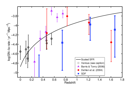
Figure 8: Type Ia SN rate from the SDF, compared to results from the literature (compiled by Neill et al. 2006). Empty circles are for Cappellaro et al. (1999), Hardin et al. (2000), Pain et al. (2002), Madgwick et al. (2003), Tonry et al. (2003), Blanc et al. (2004), and Neill et al. (2006); triangles are for Barris & Tonry (2006); filled circles are for Dahlen et al. (2004); and filled squares are for our derived SDF rate. The line shows the SFH from Hopkins & Beacom (2006), scaled to fit the $z<0.5$ points.

9 Conclusions

Large samples of high-$z$ SNe are required to resolve critical incompatibilities between recent results regarding the rates of SNe Ia, and their delay time from star formation to explosion. Here we have presented an initial sample of 33 SNe from a new survey based on deep, single-epoch, re-imaging of the $0.25~{}\mathrm{deg}^{2}$ SDF. We have demonstrated that, for SN-rate purposes, such surveys can be carried out using ground-based observations, at a fraction of the cost of space-based data, and with the potential for large samples. Using Keck spectroscopy for more than half of the host galaxies, we have shown the reliability of photometric redshifts for such data, incidentally finding the SN with the highest host spectroscopic redshift reported to date, at $z=1.564$.

The SNe were classified using a novel Bayesian photometric algorithm, using solely the SN photometry in three bands, and the host-redshift information, either photometric or spectroscopic. The photometric classification of the SNe introduces biases for which we correct using simulations. The debiasing procedure we apply to the raw sample reduces significantly the fraction of SNe Ia in the redshift bin $0.5<z<1$, which otherwise would have been heavily contaminated by CC-SNe. As discussed by Neill et al. (2006), such contamination may have affected the sample acquired by Barris & Tonry (2006), and could explain the discrepancy between their measurement of the SN Ia rate and the rates measured by Pain et al. (2002) and Neill et al. (2006).

Our resulting sample is comparable to the GOODS SN sample, and is in good agreement with it, in terms of the total numbers of SNe Ia and CC-SNe, and in terms of the redshift distribution of the CC-SN sample. However, our sample of SNe Ia shows less of a decline at high redshifts than the GOODS sample does. This trend remains when comparing the SN Ia rates we derive to those derived by GOODS. We find at redshift $z\approx 0.7$ a rate which is similar to the values determined by Pain et al. (2002), Tonry et al. (2003), and Neill et al. (2006) at $z\approx 0.5$, but barely consistent with the results of Barris & Tonry (2006) and Dahlen et al. (2004). At $z\approx 1.6$, our rate determination is consistent with the result of Dahlen et al. (2004), but about 50% higher.

These results, if confirmed by larger samples, may challenge current conclusions, based on the paucity of SNe Ia found by GOODS at high redshift, concerning the SN Ia rate and the delay time. Additional epochs on this field, already being obtained, will enlarge our SN sample to the hundreds, and will test the reality of the apparent decline in the SN Ia rate at $z\gtrsim 1$. Finally, our approaches to SN search and photometric classification are likely to become important in the era of synoptic telescopes such as Pan-STARRS (Kaiser et al. 2005) and the Large Synoptic Survey Telescope (Stubbs, Sweeney & Tyson 2004), where the sheer numbers of SNe will require new approaches to analysis.

References

- Alard (2000) Alard, C. 2000, A&AS, 144, 363
- Alard & Lupton (1998) Alard, C., & Lupton, R. H. 1998, ApJ, 503, 325
- Astier, Guy, Regnault, Pain, Aubourg, Balam, Basa, Carlberg, Fabbro, Fouchez, Hook, Howell, Lafoux, Neill, Palanque-Delabrouille, Perrett, Pritchet, Rich, Sullivan, Taillet, Aldering, Antilogus, Arsenijevic, Balland, Baumont, Bronder, Courtois, Ellis, Filiol, Gonçalves, Goobar, Guide, Hardin, Lusset, Lidman, McMahon, Mouchet, Mourao, Perlmutter, Ripoche, Tao, & Walton (2006) Astier, P. et al. 2006, A&A, 447, 31
- Autry, Probst, Starr, Abdel-Gawad, Blakley, Daly, Dominguez, Hileman, Liang, Pearson, Shaw, & Tody (2003) Autry, R. G. et al. 2003, in SPIE Proc., Vol. 4841, 525
- Barris & Tonry (2006) Barris, B. J., & Tonry, J. L. 2006, ApJ, 637, 427
- Belczynski, Bulik, & Ruiter (2005) Belczynski, K., Bulik, T., & Ruiter, A. J. 2005, ApJ, 629, 915
- Benítez (2000) Benítez, N. 2000, ApJ, 536, 571
- Bertin & Arnouts (1996) Bertin, E., & Arnouts, S. 1996, A&AS, 117, 393
- Blanton, Dalcanton, Eisenstein, Loveday, Strauss, SubbaRao, Weinberg, Anderson, Annis, Bahcall, Bernardi, Brinkmann, Brunner, Burles, Carey, Castander, Connolly, Csabai, Doi, Finkbeiner, Friedman, Frieman, Fukugita, Gunn, Hennessy, Hindsley, Hogg, Ichikawa, Ivezić, Kent, Knapp, Lamb, Leger, Long, Lupton, McKay, Meiksin, Merelli, Munn, Narayanan, Newcomb, Nichol, Okamura, Owen, Pier, Pope, Postman, Quinn, Rockosi, Schlegel, Schneider, Shimasaku, Siegmund, Smee, Snir, Stoughton, Stubbs, Szalay, Szokoly, Thakar, Tremonti, Tucker, Uomoto, Vanden Berk, Vogeley, Waddell, Yanny, Yasuda, & York (2001) Blanton, M. R. et al. 2001, AJ, 121, 2358
- Cappellaro, Evans, & Turatto (1999) Cappellaro, E., Evans, R., & Turatto, M. 1999, A&A, 351, 459
- Cappellaro, Riello, Altavilla, Botticella, Benetti, Clocchiatti, Danziger, Mazzali, Pastorello, Patat, Salvo, Turatto, & Valenti (2005) Cappellaro, E. et al. 2005, A&A, 430, 83
- Casali, Lunney, Henry, Montgomery, Burch, Berry, Laidlaw, Ives, Bridger, & Vick (2001) Casali, M. et al. 2001, in The New Era of Wide Field Astronomy, ed. R. Clowes, A. Adamson, & G. Bromage (San Francisco: ASP, Conf. Ser. Vol. 232), 357
- Coleman, Wu, & Weedman (1980) Coleman, G. D., Wu, C.-C., & Weedman, D. W. 1980, ApJS, 43, 393
- Dahlen, Strolger, Riess, Mobasher, Chary, Conselice, Ferguson, Fruchter, Giavalisco, Livio, Madau, Panagia, & Tonry (2004) Dahlen, T. et al. 2004, ApJ, 613, 189
- de Vaucouleurs (1948) de Vaucouleurs, G. 1948, Annales d’Astrophysique, 11, 247
- Faber, Phillips, Kibrick, Alcott, Allen, Burrous, Cantrall, Clarke, Coil, Cowley, Davis, Deich, Dietsch, Gilmore, Harper, Hilyard, Lewis, McVeigh, Newman, Osborne, Schiavon, Stover, Tucker, Wallace, Wei, Wirth, & Wright (2003) Faber, S. M. et al. 2003, in SPIE Proc., Vol. 4841, , 1657
- Feldmann, Carollo, Porciani, Lilly, Capak, Taniguchi, Fèvre, Renzini, Scoville, Ajiki, Aussel, Contini, McCracken, Mobasher, Murayama, Sanders, Sasaki, Scarlata, Scodeggio, Shioya, Silverman, Takahashi, Thompson, & Zamorani (2006) Feldmann, R. et al. 2006, MNRAS, 372, 565
- Fernández-Soto, Lanzetta, & Yahil (1999) Fernández-Soto, A., Lanzetta, K. M., & Yahil, A. 1999, ApJ, 513, 34
- Filippenko (1997) Filippenko, A. V. 1997, ARA&A, 35, 309
- Foley, Smith, Ganeshalingam, Li, Chornock, & Filippenko (2007) Foley, R. J., Smith, N., Ganeshalingam, M., Li, W., Chornock, R., & Filippenko, A. V. 2007, ApJ, 657, L105
- Förster, Wolf, Podsiadlowski, & Han (2006) Förster, F., Wolf, C., Podsiadlowski, P., & Han, Z. 2006, MNRAS, 368, 1893
- Freeman (1970) Freeman, K. C. 1970, ApJ, 160, 811
- Gal-Yam (2005) Gal-Yam, A. 2005, The Astronomer’s Telegram, 586, 1
- Gal-Yam & Maoz (2004) Gal-Yam, A., & Maoz, D. 2004, MNRAS, 347, 942
- Gal-Yam, Maoz, Guhathakurta, & Filippenko (2003) Gal-Yam, A., Maoz, D., Guhathakurta, P., & Filippenko, A. V. 2003, AJ, 125, 1087
- Gal-Yam, Maoz, & Sharon (2002) Gal-Yam, A., Maoz, D., & Sharon, K. 2002, MNRAS, 332, 37
- (27) Gal-Yam, A., Poznanski, D., Maoz, D., Filippenko, A. V., & Foley, R. J. 2004b, PASP, 116, 597
- (28) Gal-Yam, A. et al. 2004a, ApJ, 609, L59
- Gal-Yam, Leonard, Fox, Cenko, Soderberg, Moon, Sand, Li, Filippenko, Aldering, & Copin (2007) Gal-Yam, A. et al. 2007, ApJ, 656, 372
- Graham, Driver, Petrosian, Conselice, Bershady, Crawford, & Goto (2005) Graham, A. W., Driver, S. P., Petrosian, V., Conselice, C. J., Bershady, M. A., Crawford, S. M., & Goto, T. 2005, AJ, 130, 1535
- Greggio (2005) Greggio, L. 2005, A&A, 441, 1055
- Hillebrandt & Niemeyer (2000) Hillebrandt, W., & Niemeyer, J. C. 2000, ARA&A, 38, 191
- Ho, Filippenko, & Sargent (1997) Ho, L. C., Filippenko, A. V., & Sargent, W. L. W. 1997, ApJS, 112, 315
- Hopkins & Beacom (2006) Hopkins, A. M., & Beacom, J. F. 2006, ApJ, 651, 142
- Kaiser, fake, fake, fake, fake, fake, fake, fake, fake, fake, & fake (2005) Kaiser, N. et al. 2005, BAAS, 37, 1409
- Kashikawa, Shimasaku, Yasuda, Ajiki, Akiyama, Ando, Aoki, Doi, Fujita, Furusawa, Hayashino, Iwamuro, Iye, Karoji, Kobayashi, Kodaira, Kodama, Komiyama, Matsuda, Miyazaki, Mizumoto, Morokuma, Motohara, Murayama, Nagao, Nariai, Ohta, Okamura, Ouchi, Sasaki, Sato, Sekiguchi, Shioya, Tamura, Taniguchi, Umemura, Yamada, & Yoshida (2004) Kashikawa, N. et al. 2004, PASJ, 56, 1011 (K04)
- Kashikawa, Takata, Ohyama, Yoshida, Maihara, Iwamuro, Motohara, Totani, Nagashima, Shimasaku, Furusawa, Ouchi, Yagi, Okamura, Iye, Sasaki, Kosugi, Aoki, & Nakata (2003) —. 2003, AJ, 125, 53
- Kashikawa, Yoshida, Shimasaku, Nagashima, Yahagi, Ouchi, Matsuda, Malkan, Doi, Iye, Ajiki, Akiyama, Ando, Aoki, Furusawa, Hayashino, Iwamuro, Karoji, Kobayashi, Kodaira, Kodama, Komiyama, Miyazaki, Mizumoto, Morokuma, Motohara, Murayama, Nagao, Nariai, Ohta, Okamura, Sasaki, Sato, Sekiguchi, Shioya, Tamura, Taniguchi, Umemura, Yamada, & Yasuda (2006) —. 2006, ApJ, 637, 631
- Kinney, Calzetti, Bohlin, McQuade, Storchi-Bergmann, & Schmitt (1996) Kinney, A. L., Calzetti, D., Bohlin, R. C., McQuade, K., Storchi-Bergmann, T., & Schmitt, H. R. 1996, ApJ, 467, 38
- Knop, Aldering, Amanullah, Astier, Blanc, Burns, Conley, Deustua, Doi, Ellis, Fabbro, Folatelli, Fruchter, Garavini, Garmond, Garton, Gibbons, Goldhaber, Goobar, Groom, Hardin, Hook, Howell, Kim, Lee, Lidman, Mendez, Nobili, Nugent, Pain, Panagia, Pennypacker, Perlmutter, Quimby, Raux, Regnault, Ruiz-Lapuente, Sainton, Schaefer, Schahmaneche, Smith, Spadafora, Stanishev, Sullivan, Walton, Wang, Wood-Vasey, & Yasuda (2003) Knop, R. A. et al. 2003, ApJ, 598, 102
- Kobayashi, Tsujimoto, & Nomoto (2000) Kobayashi, C., Tsujimoto, T., & Nomoto, K. 2000, ApJ, 539, 26
- Kobayashi, Tsujimoto, Nomoto, Hachisu, & Kato (1998) Kobayashi, C., Tsujimoto, T., Nomoto, K., Hachisu, I., & Kato, M. 1998, ApJ, 503, L155
- Koekemoer, Fruchter, Hook, & Hack (2002) Koekemoer, A. M., Fruchter, A. S., Hook, R. N., & Hack, W. 2002, in The 2002 HST Calibration Workshop, ed. S. Arribas, A. Koekemoer, & B. Whitmore, 337
- Li, Wang, Van Dyk, Cuillandre, Foley, & Filippenko (2007) Li, W., Wang, X., Van Dyk, S. D., Cuillandre, J.-C., Foley, R. J., & Filippenko, A. V. 2007, ApJ, 661, 1013
- Madau, Della Valle, & Panagia (1998) Madau, P., Della Valle, M., & Panagia, N. 1998, MNRAS, 297, L17
- Mannucci, Della Valle, & Panagia (2006) Mannucci, F., Della Valle, M., & Panagia, N. 2006, MNRAS, 370, 773
- Mannucci, Della Valle, Panagia, Cappellaro, Cresci, Maiolino, Petrosian, & Turatto (2005) Mannucci, F., Della Valle, M., Panagia, N., Cappellaro, E., Cresci, G., Maiolino, R., Petrosian, A., & Turatto, M. 2005, A&A, 433, 807
- Maoz & Gal-Yam (2004) Maoz, D., & Gal-Yam, A. 2004, MNRAS, 347, 951
- Matheson, Filippenko, Li, Leonard, & Shields (2001) Matheson, T., Filippenko, A. V., Li, W., Leonard, D. C., & Shields, J. C. 2001, AJ, 121, 1648
- Muller, Reed, Armandroff, Boroson, & Jacoby (1998) Muller, G. P., Reed, R., Armandroff, T., Boroson, T. A., & Jacoby, G. H. 1998, in SPIE Proc., Vol. 3355, , 577
- Neill, Sullivan, Balam, Pritchet, Howell, Perrett, Astier, Aubourg, Basa, Carlberg, Conley, Fabbro, Fouchez, Guy, Hook, Pain, Palanque-Delabrouille, Regnault, Rich, Taillet, Aldering, Antilogus, Arsenijevic, Balland, Baumont, Bronder, Ellis, Filiol, Gonçalves, Hardin, Kowalski, Lidman, Lusset, Mouchet, Mourao, Perlmutter, Ripoche, Schlegel, & Tao (2006) Neill, J. D. et al. 2006, AJ, 132, 1126
- Nugent, Kim, & Perlmutter (2002) Nugent, P., Kim, A., & Perlmutter, S. 2002, PASP, 114, 803
- Oke & Gunn (1983) Oke, J. B., & Gunn, J. E. 1983, ApJ, 266, 713
- Oke, Cohen, Carr, Cromer, Dingizian, Harris, Labrecque, Lucinio, Schaal, Epps, & Miller (1995) Oke, J. B. et al. 1995, PASP, 107, 375
- Ouchi, Shimasaku, Okamura, Furusawa, Kashikawa, Ota, Doi, Hamabe, Kimura, Komiyama, Miyazaki, Miyazaki, Nakata, Sekiguchi, Yagi, & Yasuda (2004) Ouchi, M. et al. 2004, ApJ, 611, 660
- Pain, Fabbro, Sullivan, Ellis, Aldering, Astier, Deustua, Fruchter, Goldhaber, Goobar, Groom, Hardin, Hook, Howell, Irwin, Kim, Kim, Knop, Lee, Lidman, McMahon, Nugent, Panagia, Pennypacker, Perlmutter, Ruiz-Lapuente, Schahmaneche, Schaefer, & Walton (2002) Pain, R. et al. 2002, ApJ, 577, 120
- Panagia, Della Valle, & Mannucci (2007) Panagia, N., Della Valle, M., & Mannucci, F. 2007, submitted, astro-ph/0703409
- Peng, Ho, Impey, & Rix (2002) Peng, C. Y., Ho, L. C., Impey, C. D., & Rix, H.-W. 2002, AJ, 124, 266
- Perlmutter, Aldering, Goldhaber, Knop, Nugent, Castro, Deustua, Fabbro, Goobar, Groom, Hook, Kim, Kim, Lee, Nunes, Pain, Pennypacker, Quimby, Lidman, Ellis, Irwin, McMahon, Ruiz-Lapuente, Walton, Schaefer, Boyle, Filippenko, Matheson, Fruchter, Panagia, Newberg, Couch, & The Supernova Cosmology Project (1999) Perlmutter, S. et al. 1999, ApJ, 517, 565
- Petrosian (1976) Petrosian, V. 1976, ApJ, 209, L1
- Poznanski, Gal-Yam, Maoz, Filippenko, Leonard, & Matheson (2002) Poznanski, D., Gal-Yam, A., Maoz, D., Filippenko, A. V., Leonard, D. C., & Matheson, T. 2002, PASP, 114, 833
- Poznanski, Maoz, & Gal-Yam (2007) Poznanski, D., Maoz, D., & Gal-Yam, A. 2007, AJ, accepted, astro-ph/0610129 (P07)
- Riello & Patat (2005) Riello, M., & Patat, F. 2005, MNRAS, 362, 671
- Riess, Nugent, Gilliland, Schmidt, Tonry, Dickinson, Thompson, Budavári, Casertano, Evans, Filippenko, Livio, Sanders, Shapley, Spinrad, Steidel, Stern, Surace, & Veilleux (2001) Riess, A. G. et al. 2001, ApJ, 560, 49
- (65) —. 2004a, ApJ, 607, 665
- (66) —. 2004b, ApJ, 600, L163
- Scannapieco & Bildsten (2005) Scannapieco, E., & Bildsten, L. 2005, ApJ, 629, L85
- Schechter (1976) Schechter, P. 1976, ApJ, 203, 297
- Sersic (1968) Sersic, J. L. 1968, Atlas de Galaxias Australes (Cordoba, Argentina: Observatorio Astronomico, 1968)
- Sharon, Gal-Yam, Maoz, Filippenko, & Guhathakurta (2007) Sharon, K., Gal-Yam, A., Maoz, D., Filippenko, A. V., & Guhathakurta, P. 2007, ApJ, 660, 1165
- Shimasaku, Kashikawa, Doi, Ly, Malkan, Matsuda, Ouchi, Hayashino, Iye, Motohara, Murayama, Nagao, Ohta, Okamura, Sasaki, Shioya, & Taniguchi (2006) Shimasaku, K. et al. 2006, PASJ, 58, 313
- Strolger, Riess, Dahlen, Livio, Panagia, Challis, Tonry, Filippenko, Chornock, Ferguson, Koekemoer, Mobasher, Dickinson, Giavalisco, Casertano, Hook, Blondin, Leibundgut, Nonino, Rosati, Spinrad, Steidel, Stern, Garnavich, Matheson, Grogin, Hornschemeier, Kretchmer, Laidler, Lee, Lucas, de Mello, Moustakas, Ravindranath, Richardson, & Taylor (2004) Strolger, L.-G. et al. 2004, ApJ, 613, 200
- Stubbs, Sweeney, & Tyson (2004) Stubbs, C. W., Sweeney, D., & Tyson, J. A. 2004, BAAS, 36, 1527
- (74) Sullivan, M. et al. 2006a, AJ, 131, 960
- (75) —. 2006b, ApJ, 648, 868
- Thé, Steenman, & Alcaino (1984) Thé, P. S., Steenman, H. C., & Alcaino, G. 1984, A&A, 132, 385
- Tody (1986) Tody, D. 1986, in Proceedings of the SPIE, Vol. 627, , 733
- Tonry, Schmidt, Barris, Candia, Challis, Clocchiatti, Coil, Filippenko, Garnavich, Hogan, Holland, Jha, Kirshner, Krisciunas, Leibundgut, Li, Matheson, Phillips, Riess, Schommer, Smith, Sollerman, Spyromilio, Stubbs, & Suntzeff (2003) Tonry, J. L. et al. 2003, ApJ, 594, 1
- Yagi, Kashikawa, Sekiguchi, Doi, Yasuda, Shimasaku, & Okamura (2002) Yagi, M., Kashikawa, N., Sekiguchi, M., Doi, M., Yasuda, N., Shimasaku, K., & Okamura, S. 2002, AJ, 123, 66
- Yepes, Kates, Khokhlov, & Klypin (1997) Yepes, G., Kates, R., Khokhlov, A., & Klypin, A. 1997, MNRAS, 284, 235
- Yungelson & Livio (1998) Yungelson, L. R., & Livio, M. 1998, ApJ, 497, 168