Ab-initio calculation of phonon dispersion curves: accelerating q point convergence

Abstract

We present a scheme for the improved description of the long-range interatomic force constants in a more accurate way than the procedure which is commonly used within plane-wave based density-functional perturbation-theory calculations. Our scheme is based on the inclusion of a q point grid which is denser in a restricted area around the center of the Brillouin Zone than in the remaining parts, even though the method is not limited to an area around $\Gamma$. We have tested the validity of our procedure in the case of high-pressure phases of bulk silicon considering the bct and sh structure.

I Introduction

The calculation of vibrational properties of solids, surfaces, and nanocrystals plays an important role in the structural characterization of matter. Besides the possibility to compare the vibrational frequencies with experimental data, phonon modes can be used also to determine the structural stability of a system.Zhang et al. (2006); Li et al. (2006); Xia et al. (2005); Gaál-Nagy and Strauch (2006) This requires a reliable description of the vibrational properties of a system. Nowadays, ab-initio methods based on the density-functional perturbation theory (DFPT)Baroni et al. (2001) or frozen-phonon techniquesIhm et al. (1981) are commonly used for this purpose. With the latter the phonon frequencies can be obtained by calculating the dynamical matrix for each q point along the high-symmetry directions of the Brillouin zone (BZ), which can quite cumbersome. In the former case the dynamical matrices are computed just on a (finite) grid of q points in the irreducible wedge of the Brillouin zone (IBZ) with subsequent Fourier interpolation. Because of the computational effort of these calculations, the grid is often taken as small as possible resulting sometimes in an inaccurate description of the long-range force constants yielding erroneous frequencies especially in the low-frequency range near the $\Gamma$ point. Nevertheless, also other frequencies in the Brillouin Zone can be affected.

Considering the investigation of the thermodynamic stability of the system, an error in the description of the low-frequency area close to $\Gamma$ plays just a minor role for the calculation of the free energy. However, for the investigation of the Grüneisen parameters or the thermal expansion especially at low temperatures it is necessary to describe particularly these frequencies correctly, since their reciprocal value enter the formula.Ashcroft and Mermin (1976) Furthermore, if someone is interested in the determination of soft phonon modes, which point at the instability of structure, an exact description of the corresponding frequencies is necessary. In this context one has to mention that a wrong description of the long-range force constants may yield imaginary frequencies for a stable structure, which are interpreted as a result of a structural instability.

A possibility to overcome this problem has been given by Gonze and LeeGonze and Lee (1997) by correcting the long-range dipole-dipole interaction contribution to the force constants using a term which yields the correct non analytic behavior in the limit of small q similar to the non analytic corrections yielding the LO-TO splitting. With this procedure, the description of phonons close to $\Gamma$ is significantly improved and the required number of q points is reduced. However, this scheme is restricted to semiconductors and can not be employed in case of discrepancies at points close to the boundary of the BZ, too, at least this possibility has not been proven yet.

We have taken another approach to overcome the problem of the correct description of the long-range force constants within DFPT, which is related to the q-point convergence by introducing a mini-Brillouin Zone (mini-BZ). Inside of this mini-BZ the dynamical matrices are computed for a denser mesh of q points. The mini-BZ can be chosen around the center of the BZ but also at its boundary. These additional contributions are taken into account in the determination of the force constants. The validity of this procedure has been verified in the case of the high-pressure phases of bulk silicon: we have chosen the body-centered tetragonal structure (bct) corresponding to the $\beta$-tin and the simple hexagonal (sh) structure corresponding to the sh phase. In both cases structures beyond the range of structural stability of the phase have been selected. Our method yields an improved description of the phonon dispersion curves using less q points than the standard refinement of the grid. In detail, imaginary frequencies for the bct structure near $\Gamma$ standard procedures have been traced back to erroneous force constants whereas the soft phonon mode for the sh structure have been verified.

This article is organized as follows: In Sect. II we describe the theoretical framework of our method. Next, a short review of the technical details of our investigation is given (Sect. III). In Sect. IV we apply our procedure to the bct (Sect. IV.1) and the sh (Sect. IV.2) structure of bulk silicon, where the results are compared and discussed afterwards in Sect. IV.3. Finally we summarize and draw a conclusion (Sect. V).

II Theory

In general, the phonon frequencies $\omega({\bf q})$ at a given q point in the BZ are obtained by diagonalizing the dynamical matrix ${\bf D}_{\alpha\alpha^{\prime}}(\kappa\kappa^{\prime},{\bf q})$, i.e., by solving the equation

$$\left\|\ {\rm\bf D}_{\alpha\alpha^{\prime}}{{\rm\bf q},\kappa\ \kappa^{\prime}}-\omega^{2}({\rm\bf q})\ {\bf 1}_{3N_{\rm A}}\ \right\|=0\quad,$$ (1)

where $\kappa$, $\kappa^{\prime}$ label the sublattices (the basis atoms), $\alpha,\alpha^{\prime}$ are the cartesian coordinates, and ${\bf 1}_{3N_{\rm A}}$ is the $3N_{\rm A}\times 3N_{\rm A}$ unitary matrix for $N_{\rm A}$ atoms in the cell. We focus on the Fourier-interpolation scheme to obtain the frequencies along the high-symmetry directions of the BZ. To this end, DFPT calculations of the dynamical matrices are performed for q points on a finite, regular grid of q points. These dynamical matrices are connected with the force constants matrices $\Phi_{\alpha\alpha^{\prime}}{l\ l^{\prime}\choose\kappa\ \kappa^{\prime}}$ by a discrete Fourier transform (FT):
$\displaystyle{\bf D}_{\alpha\alpha^{\prime}}(\kappa\kappa^{\prime},{\bf q})$ $\displaystyle=$ $\displaystyle\sum_{ll^{\prime}}\Phi_{\alpha\alpha^{\prime}}{l\ l^{\prime}\choose\kappa\ \kappa^{\prime}}\times$ $\displaystyle\exp\left\{-i{\bf q}\cdot\left[{\bf R}{l\choose\kappa}-{\bf R}{l^{\prime}\choose\kappa^{\prime}}\right]\right\}\quad,$
where ${\bf R}(l,\kappa)$ is the coordinate of the $\kappa$th atom in the $l$th cell. Using the common procedure within plane-wave codes one calculates the force constants by a FT from the dynamical matrices for the q points from the discrete and finite grid and subsequently obtains the dynamical matrices for any q point by FT of the force constant matrices. However, the drawback of this procedure is that the range of the forces is connected with the q points: the choice a $l_{1}$$\times$$l_{2}$$\times$$l_{3}$ grid of q points leads to the inclusion of interatomic force constants between atoms within $l_{1}$$\times$$l_{2}$$\times$$l_{3}$ cells. In other words, assuming a finer q point grid one can extend the range of the forces included in the force constants. Thus, usually convergence tests have to be performed comparing the phonon dispersion curves for calculations based on various grids. However, the number of q points is $l_{1}\cdot l_{2}\cdot l_{3}$ in the BZ (which can be reduced by symmetry), and therefore most investigations are restricted to a smaller set of q points with a less accurate description of the long-range force constants.

The long-range force constants affect particularly the low-frequency phonons close to the $\Gamma$ point which might be wrongly described within this procedure. This problem can be overcome for semiconductors by using the method described in Ref. [Gonze and Lee, 1997]. Another possibility is to use more q points in the area close to $\Gamma$ which we have chosen here.

Instead of taking increasingly grids we have taken a denser grid just in a small area around $\Gamma$ (mini-BZ), and we assume a less dense grid outside this mini-BZ. Since the FT is based on a regular grid, we interpolate the missing dynamical matrices outside the mini-BZ by a FT from the force constants based on the coarser grid. In the following detailed description we neglect the indices $\kappa$ and $\alpha$ for simplicity, and we investigate the case $l_{1}=l_{2}=l_{3}$ only. The case $l_{1}\not=l_{2}\not=l_{3}$ follows analogously.

Assuming an $n$$\times$$n$$\times$$n$ grid, the force constants $\Phi^{nnn}$ are obtained by FT from the corresponding dynamical matrices ${\bf D}^{nnn}$ calculated within DFPT:

$${\bf D}^{nnn}({\bf q})\stackrel{{\scriptstyle\rm FT}}{{\longrightarrow}}\Phi^{nnn}\quad.$$ (3)

From these force constants $\Phi^{nnn}$ the dynamical matrices for any q point in the BZ can be calculated by a back FT, therefore also for the q points on a finer grid, e.g., a $l$$\times$$l$$\times$$l$ grid with $l>n$. Thus, one gets

$$\Phi^{nnn}\stackrel{{\scriptstyle\rm FT}}{{\longrightarrow}}{\bf D}_{\rm int}^{lll}({\bf q})\quad,$$ (4)

and also from these dynamical matrices ${\bf D}_{\rm int}^{lll}({\bf q})$ one can get again force constants $\tilde{\Phi}_{\rm int}^{lll}$ by

$${\bf D}^{lll}_{\rm int}({\bf q})\stackrel{{\scriptstyle\rm FT}}{{\longrightarrow}}\tilde{\Phi}^{lll}_{\rm int}\quad,$$ (5)

which are in this case identical to $\Phi^{nnn}$. In a next step we have performed calculations of the dynamical matrices ${\bf D}^{lll}({\bf q}\in$mini-BZ$)$ for q points of the $l$$\times$$l$$\times$$l$ grid inside the mini-BZ using the DFPT procedure. Taking these dynamical matrices and the interpolated ones outside the mini-BZ, the improved force constants $\Phi^{lll}_{\rm int}$ can be calculated by

$${\bf D}^{lll}({\bf q}\in\mbox{\rm mini-BZ})\vee{\bf D}_{\rm int}^{lll}({\bf q}\not\in\mbox{\rm mini-BZ})\stackrel{{\scriptstyle\rm FT}}{{\longrightarrow}}\Phi^{lll}_{\rm int}\quad.$$ (6)

From these force constants $\Phi^{lll}_{\rm int}$ the dynamical matrices for any q, in particular along the high-symmetry directions of the BZ, are calculated in the standard way. In the limit of very fine grids one should achieve the same results as within the procedure of Gonze and Lee.Gonze and Lee (1997) However, this method is not restricted to a mini-BZ around the $\Gamma$ point since the mini-BZ can be chosen arbitrarily. This has the advantage that also ranges of the dispersion curves far away from the $\Gamma$ point can be improved. Besides, the shape of the phonon density of states for particular spectral features can be inspected in detail.

In order to apply this scheme we have modified a postprocessing routine of the QUANTUM ESPRESSO packagehttp://www.pwscf.org in order to write out not only the frequencies but also the complete dynamical matrices after the FT. We have checked the numerical stability of the method by comparing the phonon dispersion curves based on the force constants $\Phi^{888}$ from Eq. (3) and $\tilde{\Phi}_{\rm int}^{888}$ from Eq. (5), and we have found differences in the frequencies of less than $0.25~{}{\rm cm}^{-1}$.

In the following we apply the procedure for testing purpose to the two silicon structures mentioned above and describe how to choose the mini-BZ and the required $l$$\times$$l$$\times$$l$ grid.

III Method

All calculations have been carried out with the QUANTUM ESPRESSO package.http://www.pwscf.org It is based on a plane-wave pseudopotential approach to the density-functional theory (DFT).Hohenberg and Kohn (1964); Kohn and Sham (1965) For silicon we have employed a norm-conserving pseudopotential generated following the scheme suggested by v. Barth and Car.von Barth and Car (unpublished); Corso et al. (1993) The exchange-correlation energy is described within the local-density approximation (LDA).Perdew and Zunger (1981); Ceperley and Alder (1980) We have used a kinetic-energy cutoff of 40 Ry and a 20$\times$20$\times$20 Monkhorst-Pack meshMonkhorst and Pack (1976) together with a Methfessel-Paxton smearingMethfessel and Paxton (1989) using a width of 0.03 Ry to describe the electronic (metallic) ground state of the systems. The phonon frequencies have been calculated using the DFPT schemeBaroni et al. (1987); Gianozzi et al. (1991); de Girroncoli (1995) as implemented in the QUANTUM ESPRESSO package followed by a discrete Fourier Transform as described in Sect. II.

Both, the sh and bct structures have been investigated using a common body-centered orthorhombic cell (bco, lattice constants $a\not=b\not=c$) with two atoms at $(0,0,0)$ and at $(0,0.5b,\Delta c)$ in the unit cell. The symmetry of bct requires $a=b$ and $\Delta=0.25$ whereas the symmetry of sh yields $b=\sqrt{3}c$ and $\Delta=0.5$. In fact, for sh we use a biatomic supercell although the structure of the sh phase can be described with just one atom in the sh unit cell. However, using the bco cell we have access to soft modes corresponding to the doubling of the unit cell. For details of the choice of the cell see Ref. [Gaál-Nagy and Strauch, 2006]. In this work, we have relaxed the ground-state geometry of the structure for a volume fixed to 184 $a_{\rm B}^{3}$ for both sh and bct. The equilibrium lattice constants are $c/a=0.5489$ for bct and $c/a=0.5338$ and $b/a=0.9230$ for sh. The error with respect to the ideal $b/c$ ratio of sh is negligible.

IV Results

For the application of our method we have chosen the bct structure of silicon at $V=184~{}a_{B}^{3}$ which is a volume beyond the stability range of the corresponding $\beta$-tin phase. For this structure we have found a phonon instability along the $\Gamma$-X direction of the bct BZGaál-Nagy et al. (1999, 2001) which is equivalent to the $\Gamma$-T direction of the bco BZ (see Ref. [Gaál-Nagy and Strauch, 2006]). This phonon instability turned out not to be physical. The phonons in the mentioned articles had been calculated using a 4$\times$4$\times$4 Monkhorst-Pack mesh, which was slightly insufficient to describe the frequencies in this region of the BZ properly, since calculations within DFPT of dynamical matrices at q points near $\Gamma$ have yielded only real frequencies. Because the phase space of the numerically soft modes was negligibly small, the imaginary frequencies did not affect the results for the free energy. However, we use this case to check the validity of the method described in Sect. II by the use of the mini-BZ based on a 4$\times$4$\times$4 grid outside and a 8$\times$8$\times$8 one inside the mini-BZ. A comparison of the phonon dispersion curve using the 4$\times$4$\times$4 grid plus the mini-BZ with to the one based on 8$\times$8$\times$8 mesh gives an estimate of the errors using our scheme. The bct structure is also taken to exemplify the choice of the extent of the mini-BZ. Then we apply our scheme to go beyond the 8$\times$8$\times$8 mesh for the final results.

As a second example we have chosen the sh structure of silicon at $V=184~{}a_{B}^{3}$ which is also a volume beyond the stability range of the corresponding phase, here the sh phase. Choosing a biatomic supercell, a soft phonon mode has been found at the $\Gamma$ and the S point of the bco BZ.Gaál-Nagy and Strauch (2006) Both points are equivalent to the $\Gamma$ point of the monatomic sh unit cell. The finding of a soft phonon mode at the $\Gamma$ point is in accordance with other reported results.Chang and Cohen (1984); Needs and Martin (1984); Chang and Cohen (1985) In fact, the softening at the BZ-boundary point S refer to a doubling of the sh unit cell. This is in agreement with the distortion of the biatomic supercell which contains two monatomic sh cells. Thus, this soft phonon mode is of physical origin.

Both case studies, the one with an unphysical but numerically imaginary frequencies and the one with the physically correct phonon instability are described in the following, and they are finally compared and discussed.

IV.1 Application to the bct structure of silicon

IV.1.1 Standard procedure: Increasing mesh size

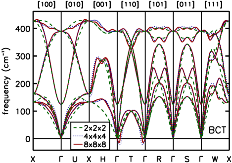
Figure 1: (Color online) Phonon dispersion curves for the bct structure at $V=184~{}{\rm a_{B}^{3}}$. Dispersion curves obtained by FT using a 2$\times$2$\times$2 mesh (dashed lines), 4$\times$4$\times$4 mesh (dotted lines), and a 8$\times$8$\times$8 mesh (solid lines).

For the bct structure at $V=184~{}a_{B}^{3}$ corresponding to a pressure of 133 kbar the frequencies along the high-symmetry directions of the bco BZ have been calculated using a 2$\times$2$\times$2, a 4$\times$4$\times$4, and a 8$\times$8$\times$8 grid. The results are shown in Fig. 1. Since the bct structure has a higher symmetry than the bco structure, the $\Gamma$-X and the $\Gamma$-R directions (bco) are equivalent to the $\Gamma$-U-X and the $\Gamma$-S directions (bct), respectively. The equivalent directions are shown mainly for completeness. The $\Gamma$-T direction with T$(\frac{1}{2},\frac{1}{2},0)$ (coordinates in units of reciprocal lattice vectors; in the following we will assume the points in the BZ always in units of reciprocal lattice vectors without mentioning it explicitly) is of particular interest because a soft phonon mode appears close to $\Gamma$ using the 4$\times$4$\times$4 mesh as visible in Fig. 1. Note, that this softening does not appear for the 2$\times$2$\times$2 grid, which is obviously insufficient to describe the phonon dispersion correctly. Increasing the mesh size, the softening remains for a 8$\times$8$\times$8 grid, however, to a minor extent. From the dispersion curves it is difficult to decide whether convergence with respect to q has been achieved for the 4$\times$4$\times$4 or not, since the the frequencies at the mesh points of the 8$\times$8$\times$8 grid are on top of the Fourier-interpolated 4$\times$4$\times$4 dispersion curves. Only for the low-frequency mode along the $\Gamma$-T direction some of the interpolated frequencies are imaginary but the 8$\times$8$\times$8 points yield just real values for the frequencies. Besides, the shape of the 8$\times$8$\times$8 Fourier-interpolated phonon curves shows just minor deviations from the 4$\times$4$\times$4 ones. Inspecting the frequencies at mesh points of the 16$\times$16$\times$16 grid, the calculated frequencies are nearly indistinguishable from the interpolated dispersion curves except along the critical $\Gamma$-T direction where all calculated points yield real frequencies, while a part of the 8$\times$8$\times$8 Fourier-interpolated phonon dispersion are imaginary.

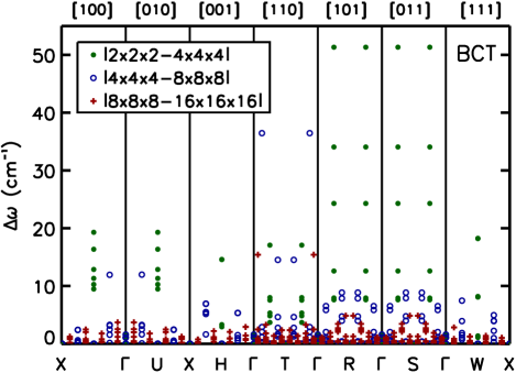
Figure 2: (Color online) Differences $\Delta\omega$ between the calculated and Fourier interpolated points along the high-symmetry directions for various meshes: $\Delta\omega=|\omega_{222}^{\rm int}-\omega_{444}^{\rm DFPT}|$ are drawn with solid symbols, $\Delta\omega=|\omega_{444}^{\rm int}-\omega_{888}^{\rm DFPT}|$ with open symbols, and $\Delta\omega=|\omega_{888}^{\rm int}-\omega_{16\,16\,16}^{\rm DFPT}|$ are with crosses (see text).

However, such a detailed study is not always possible for every system. In our case, the 2$\times$2$\times$2 mesh required the calculation of dynamical matrices at 4 q points in the IBZ, the 4$\times$4$\times$4 mesh at 13 q points, and the 8$\times$8$\times$8 mesh at 59 q points. Since the dispersion curves do not change significantly assuming a grid denser than the 4$\times$4$\times$4 except along the $\Gamma$-T direction and there only in the region close to $\Gamma$ it is not necessary to calculate all the dynamical matrices on a 8$\times$8$\times$8 or a 16$\times$16$\times$16 grid. Ultimately, the unphysical instability should be lifted. This can be achieved by applying our method described in Sect. II using a mini-BZ around $\Gamma$. The extent of the mini-BZ can be determined by inspecting the differences between the frequencies derived from the DFPT dynamical matrices $\omega^{\rm DFPT}$ and the Fourier-interpolated ones $\omega^{\rm int}$. For this purpose we have drawn in Fig. 2 the differences

$$\Delta\omega=|\omega_{nnn}^{\rm int}-\omega_{lll}^{\rm DFPT}|\quad,$$ (7)

using an $l$$\times$$l$$\times$$l$ and an $n$$\times$$n$$\times$$n$ grid with $l>n$ for the frequencies presented in Fig. 1. As mentioned above, the differences $\Delta\omega$ for the 2$\times$2$\times$2 and the 4$\times$4$\times$4 mesh are quite large. All differences decrease significantly using a finer grid, except for the points near $\Gamma$ along the $\Gamma$-T direction. Thus, the application of our method for a mini-BZ around $\Gamma$ promises an improvement of the results especially in the range of $\Gamma$-T.

IV.1.2 Approval of the present Mini-BZ method

For a first test we want to apply our method using a 4$\times$4$\times$4 grid outside the mini-BZ and an 8$\times$8$\times$8 inside. The scope of this test is to reproduce the 8$\times$8$\times$8 curves (inclusive the numerically instable mode) using a 4$\times$4$\times$4 mesh together with a Mini-BZ, since a phonon dispersion curve using a full 8$\times$8$\times$8 grid exists as a reference.

Inspecting Fig. 2, the largest deviation of the 8$\times$8$\times$8 mesh from the 4$\times$4$\times$4 mesh (open symbols in Fig. 2) of $\Delta\omega\approx 36~{}{\rm cm}^{-1}$ is found for the point $(\frac{1}{8},\frac{1}{8},0)$ along $\Gamma$-T, but also for the point $(\frac{3}{8},\frac{3}{8},0)$ the differences between the meshes are in the order of $\Delta\omega\approx 15~{}{\rm cm}^{-1}$. Besides, along X-$\Gamma$-U-X the differences are also remarkable for q points with components $q_{i}\leq\frac{1}{4}\ (i=x,y,z)$. Thus, the selection of q points up to $q_{i}\leq\frac{3}{8}$ would be a promising choice for the mini-BZ.

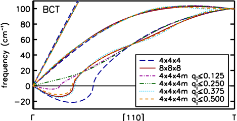
Figure 3: (Color online) Phonon dispersion curves along $\Gamma$-T using a 4$\times$4$\times$4 and a 8$\times$8$\times$8 mesh together with interpolated curves (4$\times$4$\times$4m) based on various mini BZs as denoted in the inset. Imaginary frequencies are drawn along the negative frequency axis. The cutoff for the q points is in units of reciprocal lattice vectors for $q_{i}$ with $i=x,y,z$ (see text).

In the following we have used various mini-BZs up to $q_{i}\leq\frac{1}{2}\ (i=x,y,z)$ for the interpolation (denoted as 4$\times$4$\times$4m). The results for the low-frequency range of the phonon dispersion curve along the $\Gamma$-T direction are shown in Fig. 3 in comparison with the results based on 4$\times$4$\times$4 and 8$\times$8$\times$8 grids. Note: the choice of $q_{i}\leq 1$ would make the 4$\times$4$\times$4m grid identical to the 8$\times$8$\times$8 grid. The curves for the mini-BZ with $q_{i}\leq\frac{3}{8}$ and $q_{i}\leq\frac{1}{2}$ are both very close to the curve using the full 8$\times$8$\times$8 mesh. Therefore, the choice of $q_{i}\leq\frac{3}{8}$ for the mini-BZ which has been already assumed from Fig. 2, is confirmed. Also the high-frequency region of the dispersion using an 8$\times$8$\times$8 grid is reproduced very well with this 4$\times$4$\times$4m grid (see Fig. 4). Only minor deviations appear at regions more distant from $\Gamma$ resulting from the unresolved $\Delta\omega=6.93~{}{\rm cm}^{-1}$ along X-H-$\Gamma$. However, the general improvement of the accuracy of the phonon-dispersion curve is remarkable. Note, that with this mini-BZ only 15 q points of the 8$\times$8$\times$8 have been necessary in addition to the 13 q points of the 4$\times$4$\times$4 mesh, which are much less than the 59 q points of the full 8$\times$8$\times$8 grid.

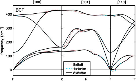
Figure 4: (color online) Comparison of the dispersion obtained from a 8$\times$8$\times$8 grid (dotted line), using the $q_{i}\leq 0.375$ mini BZ in addition to the 4$\times$4$\times$4 grid (4$\times$4$\times$4m, dashed line), and using 16$\times$16$\times$16 points in the $q_{i}\leq 0.25$ mini BZ based on force constants from the 4$\times$4$\times$4m grid (8$\times$8$\times$8m, solid line), see text. Imaginary frequencies are drawn along the negative frequency axis.

IV.1.3 Application of the Mini-BZ to denser grids

After verifying the validity of our method we want to go beyond the 8$\times$8$\times$8 mesh because of the remaining unphysical softening along $\Gamma$-T, whereas the calculated frequencies at 16$\times$16$\times$16 mesh points along the high-symmetry directions show only real values. Inspecting the differences $\Delta\omega$ in Fig. 2 again there is just a major difference of $\approx 15{\rm cm}^{-1}$ along $\Gamma$-T for q$=(\frac{1}{16},\frac{1}{16},0)$, whereas the other differences are tiny. Since along the $\Gamma$-T direction at q$=(\frac{3}{16},\frac{3}{16},0)$ there is a crucial difference of 3.3 ${\rm cm}^{-1}$, which might be important for resolving the numerical soft mode, we have tested Mini-BZs with q points up to $q_{i}\leq\frac{1}{4}$ yielding additional 29 q points. The results are denoted as 8$\times$8$\times$8m. With this mini-BZ the phonon frequencies are described accurately as shown in Fig. 4 and the softening along $\Gamma$-T has been lifted. The curves for 8$\times$8$\times$8m and 4$\times$4$\times$4m match nearly exactly indicating that convergence has been achieved. Note, that in this case the mini-BZ using 16$\times$16$\times$16 points is applied on top of the mini-BZ using 8$\times$8$\times$8 points in addition to the 4$\times$4$\times$4 mesh. In fact, we achieve convergence for 8$\times$8$\times$8m since the remaining differences $\Delta\omega$ are less than $1.25~{}{\rm cm}^{-1}$. It has to be mentioned that further improvement could be achieved using a mini-BZ close to the points T, R, and S, which is also possible within our scheme.

In summary, we have been able to obtain converged phonon dispersion curves using in total 57 q points in the IBZ which is around one sixth of the 349 q points which are required for a complete 16$\times$16$\times$16 mesh. In this way, the convergence is accelerated significantly.

IV.2 Application to the sh structure of silicon

Similarly to bct we have investigated the sh structure of bulk silicon at a volume of $V=184~{}{\rm a_{B}^{3}}$ which accords here to a pressure of 107 kbar, again beyond the range of stability of the corresponding sh phase.

IV.2.1 Standard procedure: Increasing mesh size

First, we compare the phonon-dispersion curves using the 2$\times$2$\times$2, the 4$\times$4$\times$4, and the 8$\times$8$\times$8 grid and the differences $\Delta\omega$ (see Eq.(7)) in Fig. 5. Because of the lower symmetry of the sh structure, more q points for each considered grid had to be calculated within DFPT: 5 points for 2$\times$2$\times$2, 18 for 4$\times$4$\times$4, 95 for 8$\times$8$\times$8 and 621 for 16$\times$16$\times$16. Inspecting Fig. 5, there are remarkable differences visible in the results based on a 2$\times$2$\times$2 and a 4$\times$4$\times$4 mesh and between the ones based on a 4$\times$4$\times$4 and a 8$\times$8$\times$8 mesh. This is reproduced in the graph of $\Delta\omega$. However, the variations along the $\Gamma$-T direction are rather small and the the imaginary frequencies nearly do not change the extension. In addition to the $\Gamma$ point there are significant differences around the X and the S points. Since the $\Gamma$ point and the S point are in this case equivalent, an improvement at $\Gamma$ will yield an improvement at S. Now we focus on the area around the $\Gamma$ point.

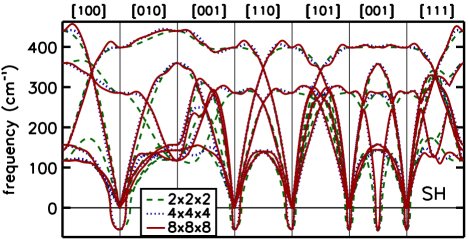
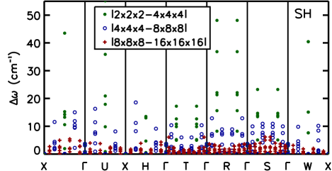
Figure 5: (color online) Phonon dispersion curves for the sh structure at $V=184~{}{\rm a_{B}^{3}}$. Upper panel: curves obtained from a 2$\times$2$\times$2 mesh (dashed lines), a 4$\times$4$\times$4 mesh (dotted lines), and a 8$\times$8$\times$8 mesh (solid lines). Imaginary frequencies are drawn along the negative frequency axis. Lower panel: differences $\Delta\omega$ for sh as in Fig. 2.

IV.2.2 Second test of the present method

Looking at the differences $\Delta\omega$ between the 4$\times$4$\times$4 and the 8$\times$8$\times$8 mesh, the choice of $q_{i}\leq\frac{3}{8}$ as for bct is not reasonable for sh since the the deviation of $\Delta\omega\leq 18.57~{}{\rm cm}^{-1}$ along the X-H-$\Gamma$ direction at q$=(0,0,\frac{7}{8})$ cannot be reduced with a mini-BZ around $\Gamma$. Nevertheless, there are differences of $\Delta\omega$ in the order of 15 ${\rm cm}^{-1}$ close to $\Gamma$ at q with $q_{i}\leq\frac{1}{4}$ which can be resolved. However, there are also significant deviations of $\approx 12~{}{\rm cm}^{-1}$ close to the R and S points. Thus we have chosen $q_{i}\leq\frac{1}{2}$. With this mini-BZ in addition to the 18 q points of the 4$\times$4$\times$4 in further 40 dynamical matrices are necessary. A comparison between the phonon dispersion curves based on the full 8$\times$8$\times$8 mesh and the one using the mini-BZ (4$\times$4$\times$4m) is presented in Fig. 6. The agreement is acceptable, only the overbending close to the X point is not described correctly due to the choice of the mini-BZ around $\Gamma$. Using an additional mini-BZ close to X would solve this problem. However, the scope here is a check of the method for a mini-BZ around $\Gamma$ analogously to the bct case (Sect. IV.1), and this region is described excellently.

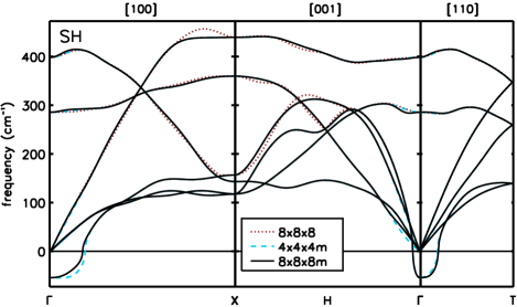
Figure 6: (color online) Comparison of the dispersion obtained from a 8$\times$8$\times$8 grid (dotted line), using the $q_{i}\leq 0.5$ mini BZ for 8$\times$8$\times$8 points in addition to the 4$\times$4$\times$4 grid (4$\times$4$\times$4m, dashed line), and using 16$\times$16$\times$16 points in the $q_{i}\leq 0.125$ mini BZ in addition to 4$\times$4$\times$4m (see text). Imaginary frequencies are drawn along the negative frequency axis.

IV.2.3 Application of the Mini-BZ to go beyond the 8$\times$8$\times$8 grid

Next, we want to go beyond the 8$\times$8$\times$8 mesh, again focussing on the region around the center of the BZ. The differences $\Delta\omega$ between the 8$\times$8$\times$8 and the 16$\times$16$\times$16 mesh show significant deviations for $q_{i}\leq\frac{1}{8}$, with a maximum of $\Delta\omega\leq 6.13~{}{\rm cm}^{-1}$ at the S point, but also for the $\Gamma$-X direction along $[100]$. In order to reduce these discrepancies and for describing especially the range of the phonon softening correctly, we have chosen $q_{i}\leq\frac{1}{8}$ for the mini-BZ by including additional 10 dynamical matrices for the calculation of the force constants. In this way, the differences $6.05~{}{\rm cm}^{-1}$ are eliminated along $\Gamma$-T. The resulting phonon-dispersion curve is presented in Fig. 6. One can notice the improvement of the results based on the 4$\times$4$\times$4m and the 8$\times$8$\times$8m grid.

Considering the numerical effort, we have used 18 dynamical matrices of the 4$\times$4$\times$4 mesh, additional 40 of the 8$\times$8$\times$8 one, and furthermore 10 of the 16$\times$16$\times$16 grid, in total 68, which is much less than the 621 dynamical matrices required for a complete 16$\times$16$\times$16 grid. Also in this case the numerical effort has been reduced drastically.

IV.3 Discussion

For both systems, the bct and the sh structure of bulk silicon, we have been able to apply successfully our scheme and we have obtained converged phonon-dispersion curves using less q points than the corresponding full mesh. Comparing the results of the bct and the sh structure, one can see that the convergence of the sh structure with respect to the q points is slower than the one of the bct structure which results in a larger choice of the mini-BZ. In particular, for bct the critical area with large variations with respect to the choice of the q mesh is around the center of the BZ whereas for sh it is around X. Since the ground state of both structures had been calculated using the same convergence parameters and the same unit cell at the same volume, the different speed of the q convergence is not due to different convergence parameters for the ground state. Therefore, one can not estimate the size of the q point grid which is required for convergence from one structure to another one even using the same cell. Thus, the q point convergence has to be tested for any structure separately. However, it was possible to confirm the soft phonon mode at $\Gamma$ for the sh structure, whereas the one of the bct structure has disappeared including enough q points around the center of the BZ. Hence, the latter phonon instability is due to an inaccurate description of the long-range force constants and thus it has only numerical origin. It would be possible to reduce the remaining discrepancies for sh around the X point using our method by applying an additional mini-BZ. However, this is beyond the scope of this article.

V Conclusions

We have presented a scheme within standard DFPT calculations for the accurate calculation of phonon dispersion curves by improving the interatomic force constants which can be applied for semiconducting systems as well as for metallic ones. Especially the long-range contribution to the force constants can be described successfully. This scheme is based on the inclusion of a denser q-point mesh in some part of the BZ (mini-BZ) and a wider one outside. The method has been applied successfully to the bct and the sh structure of bulk silicon, where the origin of a phonon instabilities has been discussed. In detail, for the bct structure the soft phonon mode has been traced back to an inaccurate description of the (long-range) force constants and the imaginary frequencies become real applying our procedure till convergence. In the case of the sh structure the soft phonon mode has been confirmed. For both cases, the number of required dynamical matrices has been reduced drastically. Whereas here the mini-BZ has been chosen around the center of the BZ, our scheme allows also a different choice. In this way, also features at the boundary of the BZ can be described more accurately. The use of our method can improve results not only for phonon dispersion curves but also for related quantities like Grüneisen parameters, thermal expansion, and the free energy.

References

- Zhang et al. (2006) L. J. Zhang, Y. L. Niu, T. Cui, Y. Li, Y. Wang, Y. M. Ma, Z. He, and G. T. Zou, J. Phys.: Condens. Matter 18, 9917 (2006).
- Li et al. (2006) Y. Li, L. Zhang, T. Cui, Y. Ma, and G. Zou, Phys. Rev. B 74, 54102 (2006).
- Xia et al. (2005) H. R. Xia, S. Q. Sun, X. F. Cheng, S. M. Dong, H. Y. Xu, L. Gao, and D. L. Cui, J. Appl. Phys. 98, 3351 (2005).
- Gaál-Nagy and Strauch (2006) K. Gaál-Nagy and D. Strauch, Phys. Rev. B 73, 014117 (2006).
- Baroni et al. (2001) S. Baroni, S. de Gironcoli, A. D. Corso, and P. Giannozzi, Rev. Mod. Phys. 73, 515 (2001).
- Ihm et al. (1981) J. Ihm, M. T. Yin, and M. L. Cohen, Solid State Commun. 37, 491 (1981).
- Ashcroft and Mermin (1976) N. W. Ashcroft and N. D. Mermin, Solid state physics (Saunders College Publishing, Fort Worth, 1976).
- Gonze and Lee (1997) X. Gonze and C. Lee, Phys. Rev. B 55, 10355 (1997).
- (9) http://www.pwscf.org.
- Hohenberg and Kohn (1964) P. Hohenberg and W. Kohn, Phys. Rev. 136 B, 864 (1964).
- Kohn and Sham (1965) W. Kohn and L. J. Sham, Phys. Rev. 140 A, 1133 (1965).
- von Barth and Car (unpublished) U. von Barth and R. Car (unpublished).
- Corso et al. (1993) A. D. Corso, S. Baroni, R. Resta, and R. Car, Phys. Rev. B 47, 3588 (1993).
- Perdew and Zunger (1981) J. P. Perdew and A. Zunger, Phys. Rev. B 23, 5048 (1981).
- Ceperley and Alder (1980) D. M. Ceperley and B. J. Alder, Phys. Rev. Lett. 45, 566 (1980).
- Monkhorst and Pack (1976) H. J. Monkhorst and J. D. Pack, Phys. Rev. B 13, 5188 (1976).
- Methfessel and Paxton (1989) M. Methfessel and A. T. Paxton, Phys. Rev. B 40, 3616 (1989).
- Baroni et al. (1987) S. Baroni, P. Giannozzi, and A. Testa, Phys. Rev. Lett. 58, 1861 (1987).
- Gianozzi et al. (1991) P. Gianozzi, S. Gironcoli, P. Pavone, and S. Baroni, Phys. Rev. B 43, 7231 (1991).
- de Girroncoli (1995) S. de Girroncoli, Phys. Rev. B 51, 6773 (1995).
- Gaál-Nagy et al. (1999) K. Gaál-Nagy, A. Bauer, M. Schmitt, K. Karch, P. Pavone, and D. Strauch, Phys. Stat. Sol. (b) 211, 275 (1999).
- Gaál-Nagy et al. (2001) K. Gaál-Nagy, M. Schmitt, P. Pavone, and D. Strauch, Comp. Mat. Sci. 22, 49 (2001).
- Chang and Cohen (1984) K. J. Chang and M. L. Cohen, Phys. Rev. B 30, R5376 (1984).
- Needs and Martin (1984) R. J. Needs and R. M. Martin, Phys. Rev. B 30, R5390 (1984).
- Chang and Cohen (1985) K. J. Chang and M. L. Cohen, Phys. Rev. B 31, 7819 (1985).