Abstract

Moduli space dynamics of multi-D-vortices from D2${\bar{\rm D}}$2 (equivalently, parallel straight D-strings from D3${\bar{\rm D}}$3) is systematically studied. For the BPS D-vortices, we show through exact calculations that the classical motion of randomly-distributed $n$ D-vortices is governed by a relativistic Lagrangian of free massive point-particles. When the head-on collision of two identical BPS D-vortices of zero radius is considered, it predicts either 90^∘ scattering or 0^∘ scattering equivalent to 180^∘ scattering. Since the former leads to a reconnection of two identical D-strings and the latter does to a case of their passing through each other, two possibilities are consistent with the prediction of string theory. It is also shown that the force between two non-BPS vortices is repulsive. Although the obtained moduli space dynamics of multi-BPS-D-vortices is exact in classical regime, the quantum effect of an F-string pair production should be included in determining the probabilities of the reconnection and the passing through for fast-moving cosmic superstrings.

1 Introduction

The development of D-branes and related string dynamics during the last decade have affected much string cosmology. Recently D- and DF-strings have attracted attentions [1] as new candidates of cosmic superstrings [2]. In understanding cosmological implications of the D(F)-strings, the description in terms of effective field theory (EFT) is efficient  [3, 4], which accommodates various wisdoms collected from the Nielsen-Olesen vortices of Abelian Higgs model [5]. In case of the Nielsen-Olesen vortices or other solitons, the derivation of the BPS limit for static multi-solitons [6] and their moduli space dynamics [7] have been two important ingredients in making the analysis tractable and systematic.

In this paper, we consider D- and DF-strings produced in the coincidence limit of D3${\bar{\rm D}}$3 as codimension-two nonperturbative open string degrees. In the context of type II string theory, we have two reliable EFT’s of a complex tachyon field reflecting the instability of D${\bar{\rm D}}$ system. One is the nonlocal action derived in boundary string field theory (BSFT) [8], and the other is Dirac-Born-Infeld (DBI) type action [9, 10]. If we restrict our interest to parallel straight D(F)-strings along one direction, the one-dimensional stringy objects can be dimensionally reduced to point-like vortices as the (cosmic) vortex-strings have been obtained from the Nielsen-Olesen vortices in Abelian Higgs model. Specifically, in the context of EFT, D0-branes from D2${\bar{\rm D}}$2 have been obtained as D-vortex configurations in (1+2)-dimensions [11, 12]. For such D0-branes, their BPS limit has been confirmed by a systematic derivation of the BPS sum rule and the reproduction of the descent relation for static single D-vortex [9] and multi-D-vortices [13, 14].

Various dynamical issues on D- and DF-strings have been addressed extensively in various contexts, for example, the collisions of DF-strings [15], the reconnection and formation of Y-junctions [1, 16], the evolutions of cosmic DF-string network [17], and the production of D(F)-strings [18]. Since the BPS limit is now attained for static multi-D-vortices from D2${\bar{\rm D}}$2 (or parallel straight multi-D-strings from D3${\bar{\rm D}}$3) in the absence of supersymmetry, the systematic study of related dynamical questions becomes tractable. The first step is to construct the classical moduli space dynamics for randomly-distributed $n$ D-vortices involving their scattering [5].

In this paper, starting from the field-theoretic static BPS and non-BPS multi-D(F)-vortex configurations, we derive systematically the moduli space dynamics for $2n$ vortex positions. The Lagrangian for randomly-distributed moving BPS D-vortices results in a relativistic Lagrangian of $n$ free point-particles of mass equal to the D0-brane tension before and after collision. The head-on collision of two identical D-vortices of zero radius predicts either 90^∘ scattering, or 0^∘ (equivalently 180^∘) scattering different from the case of BPS vortices with finite core size in the Abelian Higgs model [5]. The 90^∘ scattering leads to reconnection of two colliding identical D-strings [19], and the 0^∘ scattering suggests another possibility that two D-strings pass through each other. Two possibilities are now understood, but it cannot determine probabilities of the reconnection, $P$, and the passing, $1-P$, since our analysis is classical. The quantum correction, e.g., the production of the F-string pairs, should be taken into account in order to determine the probabilities [15]. While all the previous moduli space dynamics assumed a slow-motion [5], our result covers the whole relativistic regime. Once the probabilities are borrowed from the calculations of string theory, the result seems promising for cosmological applications of superstrings in the sense that the relativistic classical dynamics of BPS D-strings can proceed without the help of numerical analysis. A representative example is the formation and evolution of a cosmic string network [20], which has a significant cosmological implication.

The rest of the paper is organized as follows. In section 2, we introduce a DBI type effective action for D${\bar{\rm D}}$ system, and briefly recapitulate the derivation of BPS limit of static multi-D-vortices. In section 3, we derive the Lagrangian for the four coordinates of $n=2$ BPS D-vortices of zero radius without assuming a slow motion, and show 0^∘ scattering in addition to 90^∘ scattering for the head-on collision of two identical D-vortices. In section 4, we address the force between two non-BPS D-vortices. We conclude with a summary of the obtained results in section 5.

2 D${\bar{\bf D}}$ System and BPS Limit of Multi-D-vortices

The properties of D$(p-2)$ (or ${\bar{\rm D}}(p-2)$) produced from the system of D$p{\bar{\rm D}}p$ in the coincidence limit is described by an EFT of a complex tachyon field, $T=\tau\exp(i\chi)$, and two Abelian gauge fields of U(1)$\times$U(1) gauge symmetry, $A_{\mu}$ and $C_{\mu}$. A specific form of a DBI type action is [9, 10]

$$S=-{\cal T}_{p}\int d^{p+1}x\,V(\tau)\left[\,\sqrt{-\det(X^{+}_{\mu\nu})}+\sqrt{-\det(X^{-}_{\mu\nu})}\,\,\right],$$ (2.1)

where ${\cal T}_{p}$ is the tension of the D$p$-brane, and

$$X^{\pm}_{\mu\nu}=g_{\mu\nu}+F_{\mu\nu}\pm C_{\mu\nu}+({\overline{D_{\mu}T}}D_{\nu}T+{\overline{D_{\nu}T}}D_{\mu}T)/2.$$ (2.2)

We use $F_{\mu\nu}=\partial_{\mu}A_{\nu}-\partial_{\nu}A_{\mu}$, $C_{\mu\nu}=\partial_{\mu}C_{\nu}-\partial_{\nu}C_{\mu}$, and $D_{\mu}T=(\partial_{\mu}-2iC_{\mu})T$ in what follows.

In this section, we shall briefly recapitulate the derivation of BPS limit of static multi-D-strings (or DF-strings) from D3${\bar{\rm D}}$3 [13], which provides basic formulae of moduli space dynamics of the BPS objects in the subsequent section. Since the BPS limit is satisfied for parallelly-stretched D(F)-strings, we shall only consider the motion and the collision of D-strings keeping their parallel shape. Then the dynamics of parallel one-dimensional D-strings in three dimensions reduces to that of point-like D-vortices in two dimensions.

Concerned with the above discussion, let us take into account the static multi-D-vortices. We also restrict our concern to the D-vortices,

$$T=T(x^{i}),\quad(i=1,2),$$ (2.3)

without electromagnetic field, $F_{\mu\nu}=0$, throughout this paper. The effect of electromagnetic field related with DF-strings will be briefly discussed in conclusions.

Plugging (2.3) in the stress components of the energy-momentum tensor leads to

$$T^{i}_{\;j}=-\frac{2{\cal T}_{2}V}{\sqrt{1+S_{mm}-\frac{1}{2}A_{mn}^{2}}}\left[\delta_{ij}-\left(S_{ij}-\delta_{ij}S_{kk}\right)+\left(A_{ik}A_{jk}-\frac{\delta_{ij}}{2}A_{kl}^{2}\right)\right],$$ (2.4)

where

$$S_{ij}\left(A_{ij}\right)=\frac{1}{2}\left(\partial_{i}{\overline{T}}\partial_{j}T\pm\partial_{j}{\overline{T}}\partial_{i}T\right).$$ (2.5)

Reshuffling the terms, the pressure difference can be written as

$$T^{x}_{\;x}-T^{y}_{\;y}=\frac{{\cal T}_{3}V}{\sqrt{1+S_{ii}-\frac{1}{2}A_{ij}^{2}}}\left[(\overline{\partial_{x}T+i\partial_{y}T})(\partial_{x}T-i\partial_{y}T)+(\overline{\partial_{x}T-i\partial_{y}T})(\partial_{x}T+i\partial_{y}T)\right],$$ (2.6)

which vanishes when the first-order Cauchy-Riemann equation is satisfied,

$$(\partial_{x}\pm i\partial_{y})T=0,\qquad(\,\partial_{x}\ln\tau=\pm\partial_{y}\chi\;{\rm and}\;\partial_{y}\ln\tau=\mp\partial_{x}\chi\,).$$ (2.7)

Applying (2.7) to the off-diagonal stress component $T^{x}_{\;y}$, we confirm that it vanishes

$$T^{x}_{\;y} = \frac{{\cal T}_{3}V}{2\sqrt{1+S_{ii}-\frac{1}{2}A_{ij}^{2}}}\left[(\overline{\partial_{x}T\pm i\partial_{y}T})(\partial_{x}T\mp i\partial_{y}T)-(\overline{\partial_{x}T\mp i\partial_{y}T})(\partial_{x}T\pm i\partial_{y}T)\right]$$ (2.8)

$$\stackrel{{\scriptstyle(\ref{BPS})}}{{=}} 0.$$ (2.9)

Suppose that $n$ static D-vortices are located randomly in the $(x,y)$-plane. The ansatz of the tachyon field is

$$\displaystyle{T=\tau(x,y)e^{i\sum_{p=1}^{n}\theta_{p}},}\qquad\theta_{p}=\tan^{-1}\frac{y-y_{p}}{x-x_{p}},$$ (2.10)

where ${\bf x}_{p}=(x_{p},y_{p})$ $(p=1,2,...,n)$ denotes the position of each D-vortex. Inserting the ansatz (2.10) into the Cauchy-Riemann equation (2.7), we obtain the profile of the tachyon amplitude,

$$\tau(x,y)=\prod_{p=1}^{n}\tau_{{\rm BPS}}|{\bf x}-{\bf x}_{p}|.$$ (2.11)

Plugging the ansatz (2.10) and solution (2.11) into the pressure components, we obtain $-T^{x}_{\;x}=-T^{y}_{\;y}=2{\cal T}_{2}V$. Only when we take the zero-radius limit of D-vortices, $\tau_{{\rm BPS}}\rightarrow\infty$, the pressure components vanish everywhere except the points where D-vortices are located, $-T^{x}_{\;x}|_{{\bf x}={\bf x}_{p}}=-T^{y}_{\;y}|_{{\bf x}={\bf x}_{p}}=2{\cal T}_{2}$, and the Euler-Lagrange equation of the tachyon field is satisfied.

In the thin BPS limit with a Gaussian-type tachyon potential,

$$V(\tau)=\exp\left(-\frac{\tau^{2}}{\pi R^{2}}\right),$$ (2.12)

the computation of Hamiltonian for $n$ randomly-located D-vortices (2.10)–(2.11) reproduces the BPS sum rule,

$${\cal T}_{0}|n|=\int d^{2}x\;{\cal H}_{\rm BPS} = 2{\cal T}_{2}\int d^{2}x\;\lim_{\tau_{{\rm BPS}}\rightarrow\infty}V\left(\tau\right)(1+S_{xx})$$ (2.13)

$$= 2{\cal T}_{2}\int d^{2}x\;\lim_{\tau_{{\rm BPS}}\rightarrow\infty}V\left(\tau\right)S_{xx}$$ (2.14)

$$= 2\pi^{2}R^{2}{\cal T}_{2}|n|,$$ (2.15)

where ${\cal T}_{0}$ denotes the mass of unit D-vortex. The last line (2.15) means that the descent relation for codimension-two BPS branes, ${\cal T}_{0}=2\pi^{2}R^{2}{\cal T}_{2}$, is correctly obtained. Note that, for $n$ superimposed D-vortices with rotational symmetry, the integration in (2.13) yields the correct descent relation without taking the infinite $\tau_{{\rm BPS}}$ limit (or the BPS limit).

We have shown that the static multi-D-vortices in the limit of zero radius have the following properties. First, the pressures, $T^{x}_{\;x}$ and $T^{y}_{\;y}$, vanish everywhere except the positions of D-vortices, and the off-diagonal stress, $T^{x}_{\;y}$, vanishes completely. Second, the nontrivial D-vortex configuration given by the solution to the first-order Cauchy-Riemann equation also satisfies the Euler-Lagrange equation. Third, with a Gaussian-type tachyon potential, the integrated energy of static $n$ D-vortices shows that the BPS sum rule and the descent relation for codimension-two BPS branes are correctly reproduced. Therefore, the fulfillment of these necessary requirements suggests that a BPS limit of multi-D-vortices from D3${\bar{\rm D}}$3 is achieved, and that the Cauchy-Riemann equation can be identified with the first-order Bogomolnyi equation. Since supersymmetry does not exist in the D3${\bar{\rm D}}$3 system, the derivation of BPS bound is lacked differently from the usual BPS vortices in Abelian Higgs model. In this sense, the BPS properties of these multi- D-vortices (or parallel D(F)-strings) need further study.

3 Moduli Space Dynamics of Multi-D-vortices

Suppose that $n$ BPS D-vortices located randomly in the $(x,y)$-plane start to move. It is known that the classical dynamics of BPS multi-solitons is described in the context of moduli space dynamics [5, 7]. Since the BPS D-vortices are point-like objects of zero radius, the description in the moduli space seems more natural than the BPS Nielsen-Olesen vortices. In order to construct a formalism of moduli space dynamics, we should first identify the complete list of zero modes. Although we do not study the complete list of zero modes of point-like BPS D-vortices systematically by examining small fluctuations  [21], their arbitrary positions ${\bf x}_{p}$ in the $(x,y)$-plane should at least be a part of those. Different from the usual theory of a complex scalar field with spontaneously-broken global or local U(1) symmetry with a finite vacuum expectation value of the Higgs field [22], this tachyon effective action (2.1) with a runaway tachyon potential (2.12) has infinite vacuum expectation value of the tachyon amplitude and then supports neither a gapless Goldstone mode nor gauge bosons with finite mass. This reflects nonexistence of perturbative open string degrees after the D${\bar{\rm D}}$ system decays [23].

The objects of our consideration are BPS codimension-two D-vortices (D0-branes) of which classical dynamics is depicted by the motion of $n$ point particles in two-dimensions. The BPS nature predicts a free motion when they are separated, so the interaction exists only in the range of collisions, $\tau_{{\rm BPS}}|{\bf x}_{p}-{\bf x}_{q}|\leq 1$ for $p\neq q$. Let us consider the moduli space dynamics in two classes. One is for the D-vortices of which inter-distances are larger than the size of each D-vortex, $\tau_{{\rm BPS}}|{\bf x}_{p}-{\bf x}_{q}|>1$, and the other is for colliding D-vortices in the range of $\tau_{{\rm BPS}}|{\bf x}_{p}-{\bf x}_{q}|<1$.

We consider moduli space dynamics assuming that the time-dependence of fields appears in the D-vortex positions,

$${\bf x}_{p}(t)=(x_{p}(t),y_{p}(t)).$$ (3.1)

From the BPS property of point-like D-vortices, the tachyon amplitude (2.11) dictates

$$\tau=\left\{\begin{array}[]{ll}0,&\hbox{at each ${{\bf x}}_{p}$}\,,\\ \infty,&\hbox{elsewhere}.\\ \end{array}\right.$$ (3.4)

Since the BPS limit of D-vortices was attained in the absence of the gauge field $C_{\mu}$ and $A_{\mu}$, the Lagrangian of our interest from the action (2.1) is

$$L({\bf x}_{p}(t),{\dot{\bf x}}_{p}(t))$$ (3.5)

$$= \int d^{2}x\,{\cal L}(\tau,\chi,\partial_{\mu}\tau,\partial_{\mu}\chi)$$

$$= -2{\cal T}_{p}\int d^{2}xV(\tau)\sqrt{(1+S_{xx})^{2}-\left[(\partial_{t}\tau)^{2}+(\tau\partial_{t}\chi)^{2}+\tau^{2}(\partial_{t}\tau\partial_{i}\chi-\partial_{i}\tau\partial_{t}\chi)^{2}\right]}\,,$$ (3.6)

where $S_{xx}$ is given in (2.5). Since we assumed that the time-dependence appears only in the positions of D-vortices (3.1), the time-derivatives of the tachyon amplitude (2.11) and the phase (2.10) become

$$\partial_{0}\ln\tau=-\sum_{p=1}^{n}\frac{{\dot{\bf x}}_{p}(t)\cdot({\bf x}-{\bf x}_{p}(t))}{\left|{\bf x}-{\bf x}_{p}(t)\right|^{2}},\qquad\partial_{0}\chi=\sum_{p=1}^{n}\frac{\epsilon_{ij}{\dot{\bf x}_{p}^{i}}\,({\bf x}-{\bf x}_{p}(t))^{j}}{\left|{\bf x}-{\bf x}_{p}(t)\right|^{2}}.$$ (3.7)

Plugging (3.7) with the solutions (2.10)–(2.11) of the first-order Bogomolnyi equation and with their spatial derivatives into the Lagrangian (3.6), we have

$$L^{(n)}({\bf x}_{p}(t),{\dot{\bf x}}_{p}(t)) = -\frac{{\cal T}_{0}}{\pi^{2}R^{2}}\int d^{2}(\tau_{{\rm BPS}}x)\exp\left[-\frac{\left(\prod_{s_{1}=1}^{n}\tau_{{\rm BPS}}|{\bf x}-{\bf x}_{s_{1}}|\right)^{2}}{\pi R^{2}}\right]$$ (3.8)

$$\times\left[\frac{1}{\tau_{{\rm BPS}}^{2}}+\left(\prod_{s_{2}=1}^{n}\tau_{{\rm BPS}}|{\bf x}-{\bf x}_{s_{2}}|\right)^{2}\sum_{s_{3},s_{4}=1}^{n}\frac{\cos\theta_{s_{3}s_{4}}}{\tau_{{\rm BPS}}|{\bf x}-{\bf x}_{s_{3}}|\tau_{{\rm BPS}}|{\bf x}-{\bf x}_{s_{4}}|}\right]$$

$$\times\sqrt{1-\frac{\displaystyle{\left(\prod_{s_{5}=1}^{n}\tau_{{\rm BPS}}|{\bf x}-{\bf x}_{s_{5}}|\right)^{2}\sum_{p,q=1}^{n}\frac{\cos\theta_{pq}}{\tau_{{\rm BPS}}|{\bf x}-{\bf x}_{p}|\tau_{{\rm BPS}}|{\bf x}-{\bf x}_{q}|}}}{\displaystyle{\frac{1}{\tau_{{\rm BPS}}^{2}}+\left(\prod_{s_{6}=1}^{n}\tau_{{\rm BPS}}|{\bf x}-{\bf x}_{s_{6}}|\right)^{2}\sum_{s_{7},s_{8}=1}^{n}\frac{\cos\theta_{s_{7}s_{8}}}{\tau_{{\rm BPS}}|{\bf x}-{\bf x}_{s_{7}}|\tau_{{\rm BPS}}|{\bf x}-{\bf x}_{s_{8}}|}}}{\,\dot{\bf x}}_{p}\cdot{\dot{\bf x}}_{q}}\;,$$

where $\theta_{s_{i}s_{j}}$ is the angle between two vectors, $({\bf x}-{\bf x}_{s_{i}})$ and $({\bf x}-{\bf x}_{s_{j}})$. For the non-BPS D-vortices with finite $\tau_{{\rm BPS}}$, the integration over ${\bf x}$ in (3.8) looks impossible to be performed in a closed form except for the case of $n$ superimposed D-vortices, ${\bf x}_{1}={\bf x}_{2}=\cdots={\bf x}_{n}$ and ${\dot{\bf x}}_{1}={\dot{\bf x}}_{2}=\cdots={\dot{\bf x}}_{n}$,

$$L({\bf x}_{1},{\dot{\bf x}}_{1})=-n{\cal T}_{0}\left(1+\frac{1}{\tau_{{\rm BPS}}^{2}}\right)\sqrt{1-\frac{\tau_{{\rm BPS}}^{2}}{1+{\tau_{{\rm BPS}}^{2}}}{\dot{\bf x}}_{1}^{2}}\,,$$ (3.9)

which is nothing but the Lagrangian of $n$ free relativistic particles of mass ${\cal T}_{0}(1+\tau_{{\rm BPS}}^{2})/\tau_{{\rm BPS}}^{2}$ moving with a velocity $\tau_{{\rm BPS}}\,{\dot{\bf x}}_{1}/\sqrt{1+\tau_{{\rm BPS}}^{2}}\,$. If we take the BPS limit of infinite $\tau_{{\rm BPS}}$, the mass and the velocity become ${\cal T}_{0}$ and ${\dot{\bf x}}_{1}$, respectively. The result in this limit suggests a correct moduli space dynamics of randomly-distributed BPS D-vortices.

The classical motion of separated BPS objects is characterized by no interaction between any pairs of BPS solitons due to exact cancelation. Since we did not assume a slow motion in deriving the effective Lagrangian (3.8) from the field-theory one (3.5), the first candidate for the BPS configuration is the sum of $n$ relativistic free-particle Lagrangians with mass ${\cal T}_{0}$. From now on we shall show that it is indeed the case. For any pair of D-vortices, we may assume that the separation is larger than the size of each D-vortex, which is of order of $1/\tau_{{\rm BPS}}$. This assumption is valid everywhere for the BPS D-vortices obtained in the zero-radius limit, $\tau_{{\rm BPS}}\rightarrow\infty$, except for the instance of collision, which is to be considered later.

The first static part in the Lagrangian (3.6) becomes a sum of $n$ $\delta$-functions in the BPS limit as given in (2.13)–(2.15), which is the condition for BPS sum rule. Substituting it into the Lagrangian (3.8) and taking $\tau_{{\rm BPS}}\rightarrow\infty$ limit in the square root, we obtain

$$L^{(n)}({\bf x}_{p},{\dot{\bf x}}_{p}) = -{\cal T}_{0}\int d^{2}{\bar{x}}\sum_{s_{1}=1}^{n}\delta^{(2)}({\bar{\bf x}}-{\bar{\bf x}}_{s_{1}})$$

$$\times\sqrt{1-\frac{\displaystyle{\sum_{p=1}^{n}\prod\limits_{\scriptstyle s_{2}=1\atop\scriptstyle(s_{2}\neq p)}^{n}({\bar{\bf x}}-{\bar{\bf x}}_{s_{2}})^{2}\,{\dot{\bar{\bf x}}}_{p}^{2}+\sum\limits_{\scriptstyle p,q=1\atop\scriptstyle(p\neq q)}^{n}|{\bar{\bf x}}-{\bar{\bf x}}_{p}||{\bar{\bf x}}-{\bar{\bf x}}_{q}|\prod\limits_{\scriptstyle s_{2}=1\atop\scriptstyle(s_{2}\neq p,q)}^{n}({\bar{\bf x}}-{\bar{\bf x}}_{s_{2}})^{2}\cos\theta_{pq}\,{\dot{\bar{\bf x}}}_{p}\cdot{\dot{\bar{\bf x}}}_{q}}}{\displaystyle{\sum_{s_{4}=1}^{n}\prod\limits_{\scriptstyle s_{3}=1\atop\scriptstyle(s_{3}\neq s_{4})}^{n}({\bar{\bf x}}-{\bar{\bf x}}_{s_{3}})^{2}+\sum\limits_{\scriptstyle s_{4},s_{5}=1\atop\scriptstyle(s_{4}\neq s_{5})}^{n}|{\bar{\bf x}}-{\bar{\bf x}}_{s_{4}}||{\bar{\bf x}}-{\bar{\bf x}}_{s_{5}}|\prod\limits_{\scriptstyle s_{3}=1\atop\scriptstyle(s_{3}\neq s_{4},s_{5})}^{n}({\bar{\bf x}}-{\bar{\bf x}}_{s_{3}})^{2}\cos\theta_{s_{4}s_{5}}}}}$$

$$= -{\cal T}_{0}\sum_{p=1}^{n}\sqrt{1-{\dot{\bf x}}_{p}^{2}}\;,$$ (3.11)

where ${\bar{\bf x}}\equiv\tau_{{\rm BPS}}{\bf x}$, ${\bar{\bf x}_{p}}\equiv\tau_{{\rm BPS}}{\bf x}_{p}$, and ${\dot{\bar{\bf x}}}_{p}\equiv d(\tau_{{\rm BPS}}{\bf x}_{p})/d(\tau_{{\rm BPS}}t)={\dot{\bf x}}_{p}$. The resulting Lagrangian (3.11) describes $n$ relativistic free particles of mass ${\cal T}_{0}$ in the speed limit $|{\dot{\bf x}}_{p}|\leq 1$ as expected. It correctly reflects the character of point-like classical BPS D-vortices of which actual dynamics is governed by the relativistic field equation of a complex tachyon $T(t,{\bf x})$. In addition, the size of each BPS D-vortex approaches zero as $\tau_{{\rm BPS}}$ goes to infinity, and thus the description in terms of the free Lagrangian (3.11) is valid for any case of small separation between two D-vortices, i.e., $\lim_{\tau_{{\rm BPS}}\rightarrow\infty}\tau_{{\rm BPS}}|{\bf x}_{p}-{\bf x}_{q}|\rightarrow\infty$ for $|{\bf x}_{p}-{\bf x}_{q}|>0$ $(p\neq q)$.

Although the obtained result looks trivial, actually the relativistic Lagrangian of multi-BPS objects (3.5) has never been derived through systematic studies of moduli space dynamics. Traditional methods of the moduli space dynamics of multi-BPS vortices assume a slow motion of BPS solitons, and then read the metric of moduli space [7, 5]. Therefore, its relativistic regime is supplemented only by numerical analysis which solves field equations directly.

As we mentioned earlier, the obtained relativistic Lagrangian (3.5) of $n$ BPS D-vortices is free from perturbative open string degrees due to the decay of unstable D${\bar{\rm D}}$. It means that the classical dynamics of BPS D-vortices with nonzero separation can be safely described by (3.5) and should be consistent with the numerical analysis dealing with time-dependent field equations. However, the full string dynamics dictates the inclusion of F-string pairs between two D-strings and perturbative closed string degrees from the decay of D${\bar{\rm D}}$, which may affect the dynamical evolution of BPS D-vortices in quantum level. One may also ask whether or not this derivation of the relativistic Lagrangian of free particles is a consequence of DBI type action. The specific question is how much the square-root form of DBI action (2.1) affects the derivation. Although we do not have any other example to compare, the Lagrangian (3.5) backs up the validity of the DBI type action (2.1) as a tree-level Lagrangian.

Another characteristic BPS property appears in the scattering of BPS objects. That is a head-on collision of two identical spinless BPS vortices in Abelian Higgs model showing $90^{\circ}$ scattering [5, 7] which leads to the reconnection of two identical vortex-strings [19]. On the other hand, two identical D-strings can also pass through each other [15], which distinguishes the cosmic superstrings from the cosmic strings. From now on we study the dynamics of multi-BPS D-vortices when they are overlapped at the moment of collision, and address this intriguing question.

Let us discuss the head-on collision of two identical BPS D-vortices in comparison to the Nielsen-Olesen vortices in their BPS limit. For the Nielsen-Olesen vortices, the size is characterized by the inverse of the Higgs scale $v$, and is finite $\sim 1/v$ in the BPS limit ($\lambda=1$). On the other hand, the mass scale of the Lagrangian (3.11) for $n$ D-strings per unit length is characterized by the tension of the lower dimensional brane, ${\cal T}_{0}$. Meanwhile the D-vortex size is determined by $1/\tau_{\rm BPS}$ which becomes zero in the BPS limit. Therefore, the D-vortex size is different from the theory scale in the BPS limit,

$${1\over\tau_{\rm BPS}}\to 0\ll{1\over{\cal T}_{0}}.$$ (3.12)

The scattering of zero-radius vortices exhibits a very different picture from that of finite-size vortices. In the scattering of “classical” particles, the finite-size objects exhibit only one possibility which is the bouncing-back head-on collision. However, the zero-radius objects exhibit another possibility which is passing through each other owing to the zero impact parameter.

When the “quantum” concept of identical particles is taken into account, the interpretation of the scattering picture becomes somewhat different. For identical quantum particles, two particles are indistinguishable in their coalescence limit. The particles are simply superimposed, which is a solution of overlapped solitons satisfying a nonlinear wave equation. As a result, a particle sees only a half of the moduli space, so the moduli space for a particle is not a complete ${\rm R}^{2}$ but a cone as shown in Fig. 1.

For the zero-radius vortices, the apex of the cone is sharp and thus singular. At the moment of collision at the singular apex, the scattering is unpredictable. What we can consider is only the symmetry argument. There is a ${\rm Z}_{2}$ symmetry between the upper and the lower quadrant of the moduli space which is required to be kept before and after the collision. Considering the symmetry there are only two possible scattering trajectories. A vortex which climbs up the cone either overcomes the apex straightly, or bounces back. The former corresponds to the 90^∘ scattering in the physical space. Since the identical vortices are indistinguishable in the coalescence limit (at the apex), it is unpredictable if the vortex has scattered to the right or to the left. The latter bouncing-back case corresponds to the 0^∘ (equivalently 180^∘) scattering in the physical space. As Nielsen-Olesen vortices have a finite size in the BPS limit, the moduli space is a stubbed cone of which apex is smooth. The only possible geodesic motion of a vortex is overcoming straightly the apex. Therefore, there is only the 90^∘ scattering in the physical space, and the corresponding symmetry story is the same as for D-vortices.

The scattering story of vortices discussed so far can be continued for two identical straight strings. The scattering of usual cosmic strings mimics that of the Nielsen-Olesen BPS vortices. The 90^∘ scattering for vortices corresponds to the “reconnection” for cosmic strings. Since this is the only possibility for finite-size Nielsen-Olesen BPS vortices, the reconnection probability is unity. Strings never pass through each other.

The scattering picture of infinitely thin cosmic D-strings can be borrowed from the scattering of the BPS D-vortices. In addition to the reconnection as in cosmic strings, the cosmic D-strings can pass through each other with a probability $1-P$, which corresponds to the 0^∘ (180^∘) scattering for D-vortices.

The reconnection probability plays the key role in cosmologically distinguishing cosmic strings and cosmic superstrings. Beginning with the same initial configuration of the string network, cosmic superstrings evolve in a different way from cosmic strings due to non-unity $P$. Such a difference may be imprinted in the cosmic microwave background and the gravitational wave radiation. In addition, when F- and DF-strings are considered, a $Y$-junction can be possibly formed.

The computation of the probability $P$ for cosmic superstrings should be determined from string theory calculations [15]. The F-string pair production should also be included in determining $P$. When D-strings are considered, there appears an F${\bar{\rm F}}$-string pair connecting them. The energy cost of this pair production is proportional to $2\ell$ where $\ell$ is the distance between D-strings. In the coalescence limit $\ell\to 0$, the energy cost becomes zero, so the F${\bar{\rm F}}$-pair arises possibly as another zero mode of the theory. Note that this quantum level discussion is beyond our classical analysis, but we can reproduce the classical result: The scattering of two identical D-strings stretched straightly to infinity, results in either reconnection or passing through, which is different from the case of vortex-strings based on the vortices of Abelian Higgs model.

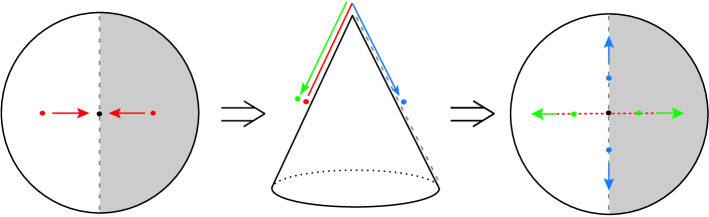
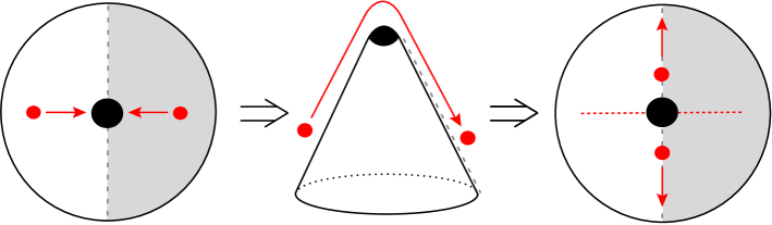
Figure 1: Scattering picture of two identical BPS D-vortices (upper panel) and of BPS Nielsen-Olesen vortices (lower panel). Since the two vortices are identical, a vortex sees only the half space (the shaded region is equivalent to the unshaded region). In addition, there is a ${\rm Z}_{2}$ symmetry between the upper and the lower quadrant. After semi-diametric dashed lines are identified, the moduli space for a vortex becomes a cone. For the zero-size D-vortices, the moduli space is a sharp cone. Considering the symmetry the scattering has two possibilities, 90^∘ scattering and 0^∘ (equivalently 180^∘) scattering. For the finite-size Nielsen-Olesen vortices, the moduli space is a stubbed cone, and there is only the 90^∘ scattering.

4 Interaction between non-BPS D-vortices

In the previous section, we considered the motion and scattering of BPS D-vortices in the context of moduli space dynamics. In the present section, we consider non-BPS D-vortex configurations in (2.10)–(2.11) with a finite $\tau_{{\rm BPS}}$, and study their dynamics and interaction between two D-vortices in the same manner based on (3.1). Note that the non-BPS configurations under consideration are given by the solutions (2.10)–(2.11) of the first-order Bogomolnyi equation (2.7). However, they are not exact solutions, but approximate solutions of the Euler-Lagrange equation. Therefore, the validity of forthcoming analysis is probably limited, and the obtained results may only be accepted qualitatively.

Since the Lagrangian (3.8) was derived for the configurations of arbitrary $\tau_{{\rm BPS}}$, it can also be employed in describing the motion and the interaction between non-BPS D-vortices. Here we restrict our interest to the case of two D-vortices $(n=2)$ since it is sufficient without loss of generality. As far as the dynamics of two D-vortices is concerned, only the relative motion is physically meaningful. Adopting the center-of-mass coordinates, we consider two identical non-BPS D-vortices at initial positions, ${\bf d}_{0}/2=(d/2,0)$ and $-{\bf d}_{0}/2=(-d/2,0)$. As time elapses, the motion of two D-vortices with size $1/\tau_{{\rm BPS}}$ is described in terms of the positions, ${\bf d}(t)/2$ and $-{\bf d}(t)/2$, with the linear momentum being conserved. Introducing rescaled variables, ${\bar{\bf d}}\equiv\tau_{{\rm BPS}}{\bf d}/(\sqrt{\pi}R)^{1/n}$ and ${\bar{t}}\equiv\tau_{{\rm BPS}}t/(\sqrt{\pi}R)^{1/n}$, the complicated Lagrangian (3.8) reduces to a simple one of the single particle

$$L^{(2)}({\bar{\bf d}}(t),{\dot{\bar{\bf d}}}(t))=-\frac{4{\cal T}_{0}}{\pi}\int d^{2}{\bar{x}}\,e^{-|{\bar{\bf x}}-{\bar{\bf d}}/2|^{2}|{\bar{\bf x}}+{\bar{\bf d}}/2|^{2}}\left(d_{\tau}^{2}+{\bar{\bf x}}^{2}\right)\sqrt{1-\frac{({\bar{\bf d}}/2)^{2}}{d_{\tau}^{2}+{\bar{\bf x}}^{2}}{\dot{\left(\frac{{\bar{\bf d}}}{2}\right)}}^{2}}\,,$$ (4.1)

where $d_{\tau}\equiv 1/2\pi^{\frac{1}{4}}\sqrt{R}\,\tau_{{\rm BPS}}$ and ${\dot{\bar{\bf d}}}={\dot{\bf d}}$.

The first step to understand the mutual interaction between two D-vortices is to investigate the potential energy,

$$U^{(2)}({\bar{\bf d}}) \equiv -\left.L^{(2)}({\bar{\bf d}},{\dot{\bar{\bf d}}})\right|_{{\dot{\bar{\bf d}}}={\mathbf{0}}}$$ (4.2)

$$= 2{\cal T}_{0}\left[1+\sqrt{\pi}\;d_{\tau}^{2}\;\exp\left(-\frac{{\bar{\bf d}}^{4}}{32}\right)\emph{I}_{0}\left(\frac{{\bar{\bf d}}^{4}}{32}\right)\right],$$ (4.3)

where $\emph{I}_{0}$ is the modified Bessel function.

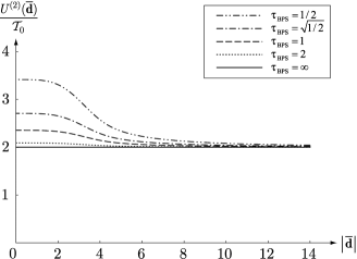
Figure 2: Potential energy $U^{(2)}({\tilde{d}})$ for various $\tau_{{\rm BPS}}$’s.

As shown in Fig. 2, the first constant piece in (4.3) is independent of $\tau_{{\rm BPS}}$ and stands for the rest mass of two D-vortices, $2{\cal T}_{0}$, in the BPS limit ($\tau_{{\rm BPS}}=\infty$). The second distance-dependent term is a monotonically-decreasing function. Its maximum value for the superimposed D-vortices is $U^{(2)}({\bar{\bf d}}=0)-2{\cal T}_{0}={\cal T}_{0}/2R\tau_{{\rm BPS}}^{2}$ which vanishes in the BPS limit of infinite $\tau_{{\rm BPS}}$. This $\tau_{{\rm BPS}}$-dependent potential energy shows a repulsive short-distance interaction between two non-BPS D-vortices. Fig. 2 also shows that as $\tau_{{\rm BPS}}$ increases the system approaches the BPS limit very rapidly.

In the current system, the conserved mechanical energy is nothing but the Hamiltonian, $E^{(2)}({\bar{\bf d}},{\dot{\bar{\bf d}}})=(\partial L^{(2)}/\partial{\dot{\bar{\bf d}}})\cdot{\dot{\bar{\bf d}}}-L^{(2)}$. The kinetic energy is then given by

$$K^{(2)}({\bar{\bf d}},{\dot{\bar{\bf d}}}) \equiv E^{(2)}({\bar{\bf d}},{\dot{\bar{\bf d}}})-U^{(2)}({\bar{\bf d}})$$ (4.4)

$$= \frac{4{\cal T}_{0}}{\pi}\int d^{2}{\bar{x}}\,e^{-|{\bar{\bf x}}-{\bar{\bf d}}/2|^{2}|{\bar{\bf x}}+{\bar{\bf d}}/2|^{2}}\Bigg{[}\frac{1}{\sqrt{1-\frac{({\bar{\bf d}/2)}^{2}}{d_{\tau}^{2}+{\bar{\bf x}}^{2}}{\dot{\left(\frac{{\bar{\bf d}}}{2}\right)}}^{2}}}-1\Bigg{]}.$$

To understand the motion in detail, the spatial integration over ${\bar{\bf x}}$ should be performed for the kinetic term (4.4), but it is impossible when the function inside the square root becomes negative,

$$0\leq{\bar{\bf x}}^{2}<{\left(\frac{{\bar{\bf d}}}{2}\right)}^{2}{\dot{\left(\frac{{\bar{\bf d}}}{2}\right)}}^{2}-d_{\tau}^{2}.$$ (4.5)

If the distance $|{\bar{\bf d}}/2|$ and the speed $|{\dot{\bar{\bf d}}}/2|$ are respectively smaller than the characteristic length $d_{\tau}$ and the speed of light (unity in our unit system), the integrand becomes imaginary and the moduli space dynamics is not validly described anymore. As expected, for non-BPS D-vortices, this formalism is applicable only to the regime of long distance and slow motion, so-called the IR region. As $\tau_{{\rm BPS}}$ approaches infinity in the BPS limit, $d_{\tau}$ becomes zero. Therefore, the integration can be performed for all $|{\bar{\bf d}}/2|$ and $|{\dot{\bar{\bf d}}}/2|$. (The UV physics is probed in the BPS limit.)

It is necessary to consider the nonrelativistic limit of two slowly-moving non-BPS D-vortices with $|{\dot{\bar{\bf d}}}/2|\ll 1$ in order to investigate the motions in detail. When the speed is low enough, the nonrelativistic Lagrangian is given from (4.1) as $L^{(2)}\approx(M^{(2)}/2)({\dot{\bar{\bf d}}}/2)^{2}-U^{(2)}$. Here the reduced mass function $M^{(2)}$ is

$$M^{(2)}({\bar{\bf d}})=2{\cal T}_{0}\frac{\sqrt{\pi}}{4}\;{\bar{\bf d}}^{2}\exp\left(-\frac{{\bar{\bf d}}^{4}}{32}\right)\emph{I}_{0}\left(\frac{{\bar{\bf d}}^{4}}{32}\right).$$ (4.6)

Figure 3: Mass function $M^{(2)}({\bar{\bf d}})$ of two D-vortices in nonrelativistic motion.

As shown in Fig. 3, the mass function (4.6) starts from zero and increases to a maximum value at a finite $d_{{\rm max}}$. Then it decreases rapidly and asymptotes to 2 at infinity. Although the mass formula itself (4.6) is independent of $\tau_{{\rm BPS}}$, the inequality (4.5) puts a limit on the validity. It is valid only at much larger distances than $d_{\tau}$. Note also that the region of drastic mass change, where two D-vortices are overlapped, should be excluded in reading detailed physics.

The speed of a D-vortex is obtained from the nonrelativistic mechanical energy $E^{(2)}$,

$$\left|\;\frac{{\dot{\bar{\bf d}}}}{2}\;\right|=\frac{1}{{\bar{\bf d}}}\sqrt{\frac{4(E^{(2)}/{\cal T}_{0}-2)}{\sqrt{\pi}\exp\left(-\frac{{\bar{\bf d}}^{4}}{32}\right)\emph{I}_{0}\left(\frac{{\bar{\bf d}}^{4}}{32}\right)}-\frac{2}{\sqrt{\pi}R\tau_{{\rm BPS}}^{2}}}\;.$$ (4.7)

When the initial speed $|{\dot{\bar{\bf d}}}_{0}/2|$ is lower than the critical speed $1/\sqrt{2R\tau_{\rm BPS}^{2}}\;$ for non-BPS D-vortices with finite $\tau_{\rm BPS}$, the D-vortex turns back at a finite turning point due to the repulsive potential (4.3). If the initial speed $|{\dot{\bar{\bf d}}}_{0}/2|$ exceeds the critical speed, two identical D-vortices can collide at the origin but this discussion in the region near the origin is not valid under the nonrelativistic and long-distance approximation.

In studying the interaction and relative motion of identical non-BPS vortices, we considered only two D-vortices. Extensions to the cases of arbitrary number of non-BPS D-vortices are straightforward, at least formally. Again, it should be noted that it is difficult to perform explicitly the spatial integration for the Lagrangian (3.8).

5 Conclusions

In this paper, we investigated the dynamics of D-strings produced in the coincidence limit of D3${\bar{\rm D}}$3 as codimension-two nonperturbative open string degrees. The model is described by a DBI type effective action with a complex tachyon field. It was shown in [13] that the infinitely thin static tachyon profile with a Gaussian-type potential reproduces the BPS configuration with the correct BPS sum rule and descent relation. Since the D-strings are parallelly stretched, their transverse dynamics is described by point-like BPS D-vortices in two dimensions.

In this work, we investigated the dynamics of such $n$ randomly-distributed BPS D-vortices assuming that their positions are time-dependent. We found that the classical moduli space dynamics before and after collision is governed by a simple Lagrangian $L^{(n)}({\bf x}_{p},{\dot{\bf x}}_{p})=-{\cal T}_{0}\sum_{p=1}^{n}\sqrt{1-{\dot{\bf x}}_{p}^{2}}$ which describes $n$ free relativistic point particles with the mass given by the D0-brane tension. Such a relativistic Lagrangian of multi-BPS objects has never been derived through systematic studies of moduli space dynamics. We also studied the classical scattering of identical D-vortices. Different from the Abelian Higgs BPS vortices with finite thickness, we could show that the head-on collision of two identical D-vortices with zero radius exhibits either 90^∘ scattering or 0^∘ even in the relativistic case.

Since the BPS limit is achieved in the zero-radius limit for D-vortices, the obtained moduli dynamics possibly describes the classical dynamics of the BPS D(F)-strings more accurately even for the motion of high speed. Dynamics of cosmic superstrings can be deduced analogously from the aforementioned vortex dynamics. After the collision, the identical cosmic D-strings can either reconnect with a probability $P$, or pass through without inter-commute with $1-P$. The computation of the reconnection probability $P$ requires string theory calculations. This picture is very different from that of the usual Nielsen-Olesen cosmic strings which always reconnect after the collision. In D-string collisions, the F-string pair production should also be considered since the energy cost of such a pair production becomes zero in the coincidence limit of D-strings. This F-string pair may provide another zero mode in the scheme of moduli space dynamics.

We studied the interaction of two D-vortices for the non-BPS case in which the vortices have a finite size. We could show that the effective potential for the motion exhibits a repulsive force. Slowly incoming D-vortices will eventually bounce back. As the vortex size approaches zero, the effective potential becomes flatter, and eventually becomes completely flat which describes the noninteracting BPS limit.

What we obtained shows a possibility for treating the BPS objects and their dynamics from non-BPS systems without supersymmetry, and thus further study to this direction is needed. In addition, it must be an evidence for the validity of the DBI type effective action at least in the classical level. Although the derivation of the relativistic Lagrangian for free particles (3.5) seems unlikely in the context of BSFT due to the complicated derivative terms, it is worth tackling to check this point explicitly.

Our analysis is valid only for the straight D-strings and their dynamics along transverse directions. Therefore, the next step is to extend the analysis to the thin D(F)-strings of arbitrarily deformed shapes. When an electric field ($E_{z}$) is turned on, D-strings become DF-strings. When two DF-strings collide, they are known to form a Y-junction [1, 15, 16]. Although the static BPS DF-configuration was obtained in the same manner as the BPS D-strings [13, 14], the scattering of such DF-strings is probably more complicated, and will not be simply described by what have been investigated here for D-strings.

Although there do not exist perturbative zero modes from open string side, massless closed string degrees are produced including graviton, dilaton, and antisymmetric tensor field. These may affect much on the dynamics of D(F)-strings as was done in the case of global U(1) strings [24]. In a relation to the string cosmology based on the KKLMMT setting, the BPS nature of D(F)-strings in a warped geometry is an intriguing subject [25].

References

- [1] E. J. Copeland, R. C. Myers and J. Polchinski, “Cosmic F- and D-strings,” JHEP 0406, 013 (2004) [arXiv:hep-th/0312067]; For a review, see J. Polchinski, “Introduction to cosmic F- and D-strings,” arXiv:hep-th/0412244.
- [2] E. Witten, “Cosmic superstrings,” Phys. Lett. B 153, 243 (1985).
- [3] A. Vilenkin and E. P. S. Shellard, Cosmic strings and other topological defects, (Cambridge University Press, 1984).
- [4] T. W. B. Kibble, “Cosmic strings reborn?,” arXiv:astro-ph/0410073.
- [5] For a review, see N. Manton and P. Sutcliffe, Topological solitons, (Cambridge University Press, 2004).
- [6] E. B. Bogomolny, “Stability of classical solutions,” Sov. J. Nucl. Phys. 24, 449 (1976) [Yad. Fiz. 24, 861 (1976)].
- [7] E. P. S. Shellard and P. J. Ruback, “Vortex scattering in two-dimensions,” Phys. Lett. B 209, 262 (1988); P. J. Ruback, “Vortex string motion in the Abelian Higgs model,” Nucl. Phys. B 296, 669 (1988); T. M. Samols, “Hermiticity of the metric on vortex moduli space,” Phys. Lett. B 244, 285 (1990); “Vortex scattering,” Commun. Math. Phys. 145, 149 (1992); E. Myers, C. Rebbi and R. Strilka, “A study of the interaction and scattering of vortices in the Abelian Higgs (or Ginzburg-Landau) model,” Phys. Rev. D 45, 1355 (1992).
- [8] P. Kraus and F. Larsen, “Boundary string field theory of the DD-bar system,” Phys. Rev. D 63, 106004 (2001) [arXiv:hep-th/0012198]; T. Takayanagi, S. Terashima and T. Uesugi, “Brane-antibrane action from boundary string field theory,” JHEP 0103, 019 (2001) [arXiv:hep-th/0012210].
- [9] A. Sen, “Dirac-Born-Infeld action on the tachyon kink and vortex,” Phys. Rev. D 68, 066008 (2003) [arXiv:hep-th/0303057].
- [10] M. R. Garousi, “D-brane anti-D-brane effective action and brane interaction in open string channel,” JHEP 0501, 029 (2005) [arXiv:hep-th/0411222].
- [11] N. T. Jones and S. H. H. Tye, “An improved brane anti-brane action from boundary superstring field theory and multi-vortex solutions,” JHEP 0301, 012 (2003) [arXiv:hep-th/0211180].
- [12] Y. Kim, B. Kyae and J. Lee, “Global and local D-vortices,” JHEP 0510, 002 (2005) [arXiv:hep-th/0508027]; I. Cho, Y. Kim and B. Kyae, “DF-strings from D3 D3-bar as cosmic strings,” JHEP 0604, 012 (2006) [arXiv:hep-th/0510218].
- [13] T. Kim, Y. Kim, B. Kyae and J. Lee, “Cosmic D- and DF-strings from D3Dbar3: Black Strings and BPS Bound,” arXiv:hep-th/0612285.
- [14] G. Go, A. Ishida and Y. Kim, “BPS limit of multi- D- and DF-strings in boundary string field theory,”Phys. Lett. B 651, 394 (2007) [arXiv:hep-th/0703144].
- [15] M. G. Jackson, N. T. Jones and J. Polchinski, “Collisions of cosmic F- and D-strings,” JHEP 0510, 013 (2005) [arXiv:hep-th/0405229].
- [16] E. J. Copeland, T. W. B. Kibble and D. A. Steer, “Collisions of strings with Y junctions,” Phys. Rev. Lett. 97, 021602 (2006) [arXiv:hep-th/0601153]; “Constraints on string networks with junctions,” Phys. Rev. D 75, 065024 (2007) [arXiv:hep-th/0611243].
- [17] S. H. Tye, I. Wasserman and M. Wyman, “Scaling of multi-tension cosmic superstring networks,” Phys. Rev. D 71, 103508 (2005) [Erratum-ibid. D 71, 129906 (2005)] [arXiv:astro-ph/0503506]; E. J. Copeland and P. M. Saffin, “On the evolution of cosmic-superstring networks,” JHEP 0511, 023 (2005) [arXiv:hep-th/0505110]; M. Hindmarsh and P. M. Saffin, “Scaling in a SU(2)/Z(3) model of cosmic superstring networks,” JHEP 0608, 066 (2006) [arXiv:hep-th/0605014].
- [18] S. Sarangi and S. H. H. Tye, “Cosmic string production towards the end of brane inflation,” Phys. Lett. B 536, 185 (2002) [arXiv:hep-th/0204074]; G. Dvali and A. Vilenkin, “Formation and evolution of cosmic D-strings,” JCAP 0403, 010 (2004) [arXiv:hep-th/0312007].
- [19] E. P. S. Shellard, “Cosmic string interactions,” Nucl. Phys. B 283, 624 (1987); “Understanding Intercommuting,” MIT-CTP-1683, Proc. of Yale Workshop: Cosmic Strings: The Current Status, New Haven, CT, May 6-7, 1988; R. A. Matzner, “Interaction of U(1) cosmic strings: numerical intercommutation,” Comput. Phys. 2, 51 (1989).
- [20] T. W. B. Kibble, “Evolution of a system of cosmic strings,” Nucl. Phys. B 252, 227 (1985) [Erratum-ibid. B 261, 750 (1985)]; T. Vachaspati and A. Vilenkin, “Evolution of cosmic networks,” Phys. Rev. D 35, 1131 (1987).
- [21] E. J. Weinberg, “Multivortex solutions of the Ginzburg-Landau equations,” Phys. Rev. D 19, 3008 (1979).
- [22] R. L. Davis, “Goldstone bosons in string models of galaxy formation,” Phys. Rev. D 32, 3172 (1985); “Cosmic axions from cosmic strings,” Phys. Lett. B 180, 225 (1986).
- [23] For a review, see A. Sen, “Tachyon dynamics in open string theory,” Int. J. Mod. Phys. A 20, 5513 (2005) [arXiv:hep-th/0410103].
- [24] A. Vilenkin, “Gravitational field of vacuum domain walls and strings,” Phys. Rev. D 23, 852 (1981).
- [25] H. Firouzjahi, L. Leblond and S. H. Henry Tye, “The (p,q) string tension in a warped deformed conifold,” JHEP 0605, 047 (2006) [arXiv:hep-th/0603161]; S. Thomas and J. Ward, “Non-Abelian (p,q) strings in the warped deformed conifold,” JHEP 0612, 057 (2006) [arXiv:hep-th/0605099]; H. Firouzjahi, “Dielectric (p,q) strings in a throat,” JHEP 0612, 031 (2006) [arXiv:hep-th/0610130].