Constraints on oscillating dark energy models

Abstract

The oscillating scenario of route to Lambda was recently proposed by us Hrycyna and Szydlowski (2007) as an alternative to a cosmological constant in a explanation of the current accelerating universe. In this scenario phantom scalar field conformally coupled to gravity drives the accelerating phase of the universe. In our model $\Lambda$CDM appears as a global attractor in the phase space. In this paper we investigate observational constraints on this scenario from recent measurements of distant supernovae type Ia, $H(z)$ observational data, CMB R shift and BAO parameter. The Bayesian methods of model selection are used in comparison the model with concordance $\Lambda$CDM one as well as with model with dynamical dark energy parametrised by linear form. We conclude that $\Lambda$CDM is favoured over FRW model with dynamical oscillating dark energy. Our analysis also demonstrate that FRW model with oscillating dark energy is favoured over FRW model with decaying dark energy parametrised in linear way.

I Introduction

Observations of distant supernovae type Ia still consistently suggest that the universe is in a accelerating phase of expansion Astier et al. (2006); Riess et al. (1998); Davis et al. (2007). These confirmations are supported by CMB observations which indicate that universe is almost spatially flat Spergel et al. (2007) and that the amount of matter in the universe calculated from galaxy clustering is not enough to account for this flatness Cole et al. (2005); Tegmark et al. (2004). These observational facts regarded on the background of standard general relativity indicate that about $2/3$ of total energy of the universe today being a dark energy with negative pressure which is responsible for the current accelerated expansion if the strong energy condition is violated.

There are many candidates for dark energy description (Copeland et al., 2006, and references therein). Here we consider dark energy in the form of phantom scalar field $\psi$ with the quadratic potential function $U(\psi)$ for simplicity of presentation. The scalar field is conformally coupled to gravity. In our previous work it has been demonstrated that for generic class of initial conditions the equation of state parameter $w_{\text{eff}}=p_{\text{eff}}/\rho_{\text{eff}}$ approaches $-1$ value through the damping oscillations around this mysterious value. Hence theoretically appeared the possibility to solve the cosmological constant problem where the smallness of of cosmological constant does not require fine tuning of model parameters.

Here we use different astronomical observations to confront the model with the observational data. In this paper we use SNIa data and other tests like CMB R shift, BAO and $H(z)$ data obtained from differential ages of galaxies Simon et al. (2005). Bayesian statistics is used to constrain a set of model parameters. In the constraining the model parameters we perform combined analysis with CMB R shift parameter as calculated by Wang and Mukherjee Wang and Mukherjee (2006) for WMAP 3 Spergel et al. (2007). The main question addressing in this paper is whether data sets to favour an evolving in oscillatory way dark energy model over $\Lambda$CDM one. Using Bayesian framework of model selection we also compare oscillating parametrisation with other most popular linear in scale factor $a$ parametrisation.

Guo, Ohta and Zhang Guo et al. (2005) developed theoretical method of reconstruction of the quintessence potential directly from the effective equation of state parameter $w(z)$ for minimally coupled scalar field. This method can be extended to the case of non-minimally coupled scalar field.

II Oscillating dark energy model

Investigations of different dark energy models Copeland et al. (2006) are hindered by lack of alternatives to the effective cosmological constant model Crittenden et al. (2007). The simple step toward more realistic description is that the dark energy might vary in time. Usually the form of $w(z)$ is a priori assumption to remove some degeneration problem in analysis of constraints on model parameters from observational data. However may happened that assumed form of parametrisation of the dark energy equation of state is incompatible with true dynamics which determine $w(z)$ itself. We propose to determine corresponding form of $w(z)$ directly from the dynamical behaviour in the vicinity of stable critical point representing effective model $\Lambda$CDM. From the dynamical systems methods we know that the system in the phase space can be good approximated by its linear part Perko (1991). Then we solve differential equation determining $w_{X}(z)$. As a result we obtain Hrycyna and Szydlowski (2007)

$$w_{X}(z)=-1+(1+z)^{3}\bigg{\{}C_{1}\cos(\ln(1+z))+C_{2}\sin(\ln(1+z))\bigg{\}}$$ (1)

for phantom scalar field non-minimally (conformally) coupled to gravity Faraoni (2001). Note that a single scalar field model with general Lagrangian $L=L(\phi,\partial_{\mu}\phi\partial^{\mu}\phi)$ will not be able to have $w$ crossing $-1$ Bonvin et al. (2006) and to realize that one must introduce non-minimal coupling or modification of Einstein gravity.

We consider conformally coupled phantom scalar field with $p_{\psi}$ and $\rho_{\psi}$ given by

$$p_{\psi} =-\frac{1}{2}\dot{\psi}^{2}-U(\psi)+\xi\Big{[}2H(\psi^{2})\dot{}+(\psi^{2})\ddot{}\Big{]}+\xi\Big{[}2\dot{H}+3H^{2}\Big{]}\psi^{2},$$

$$\rho_{\psi} =-\frac{1}{2}\dot{\psi}^{2}+U(\psi)-3\xi H^{2}\psi^{2}-3\xi H(\psi^{2})\dot{},$$

where dot denotes differentiation with respect to cosmological time.

From eq.(1), instead of most popular linear parametrisation, we obtain model with characteristic crossing of $w_{X}=-1$ “phantom divide”, thereby the violation of weak energy condition infinite times in the past.

With the help of formula (1) one can simply calculate energy density for dark energy $\rho_{\Lambda}$

$$\rho_{\Lambda}=\rho_{\Lambda,0}\exp(-D_{2})\exp{\bigg{(}(1+z)^{3}\Big{[}D_{1}\sin(\ln(1+z))+D_{2}\cos(\ln(1+z))\Big{]}\bigg{)}},$$ (2)

where $D_{1}=0.3(C_{1}+3C_{2})$ and $D_{2}=0.3(3C_{1}-C_{2})$. It is interesting that some special cases of this dark energy parametrisation are explored in probing for dynamics of dark energy Zhao et al. (2007); Hooper and Dodelson (2007).

Let us consider flat FRW model filled with dark energy with density $\rho_{\Lambda}$, dust matter (baryonic and dark) and radiation. For further analysis of constraints from cosmography it would be useful to write Friedmann first integral on $H^{2}$, where $H$ is the Hubble’s parameter

$$H=H_{0}\sqrt{\Omega_{\Lambda,0}\exp(-D_{2})\exp{\bigg{(}(1+z)^{3}\Big{[}D_{1}\sin(\ln(1+z))+D_{2}\cos(\ln(1+z))\Big{]}\bigg{)}}+\Omega_{m,0}(1+z)^{3}+\Omega_{r,0}(1+z)^{4}},$$ (3)

where $\Omega_{r,0}\simeq 0.5*10^{-4}$ is fixed and $\Omega_{\Lambda,0}=1-\Omega_{m,0}-\Omega_{r,0}$. $D_{1}$, $D_{2}$ and $\Omega_{m,0}$ are free parameters which should be fitted from observational data.

III Constraints from SNIa, SDSS, CMB and H(z) observations

To constrain the unknown values of model parameters we used the set of $N=192$ SNIa data Riess et al. (2007); Davis et al. (2007); Wood-Vasey et al. (2007). Here we based on the standard relation between the apparent magnitude ($m$) and luminosity distance ($d_{L}$): $m-M=5\log_{10}D_{L}+\mathcal{M}$, where $M$ is the absolute magnitude of SNIa, $\mathcal{M}=-5\log_{10}H_{0}+25$ and $D_{L}=H_{0}d_{L}$. The luminosity distance depends on the considered cosmological model and with assumption that $k=0$ is given by $d_{L}=(1+z)c\int_{0}^{z}\frac{dz^{\prime}}{H(z^{\prime})}$.
Posterior probability for model parameters (after marginalization over nuisance parameter - $H_{0}$ with the assumption that prior probability for this parameter is flat within the interval $<60,80>$) has the following form

$$P(\bar{\theta}|M,D)\propto\int\big{(}\pi(\bar{\theta}|M)\exp\left[-0.5\chi^{2}_{SN}(\bar{\theta})\right]\big{)}dH_{0},$$ (4)

where $\chi^{2}_{SN}(\bar{\theta})=\sum_{i=1}^{N}\left(\frac{\mu_{i}^{obs}-\mu_{i}^{th}}{\sigma_{i}}\right)^{2}$, $\mu_{i}^{obs}=m_{i}-M$, $\mu_{i}^{th}=5\log_{10}D_{Li}+\mathcal{M}$, $\pi(\bar{\theta}|M)$ is the prior probability for model parameters and $\bar{\theta}=(\Omega_{m,0},D_{1},D_{2})$. Here we assumed flat prior for model parameters within the interval: $\Omega_{m,0}\in<0,1>$, $D_{1}\in<-1,1>$, $D_{2}\in<-1,1>$.

The best fit values for model parameters (the mode of the posterior probability) are the same as the best fit values obtained by $\chi^{2}$ minimization within the interval for parameters assumed before. Results, i.e. values for model parameters obtained via $\chi^{2}$ minimization procedure are gathered in Table 1.
Posterior probabilities for model parameters defined in the following way

$$P(\Omega_{m,0}|M,D)=\int\int P(\bar{\theta}|M,D)dD_{1}dD_{2}$$

$$P(D_{1}|M,D)=\int\int P(\bar{\theta}|M,D)d\Omega_{m,0}dD_{2}$$

$$P(D_{2}|M,D)=\int\int P(\bar{\theta}|M,D)d\Omega_{m,0}dD_{1}$$

are presented on Figure 1. The values of the mean for such distributions together with $68\%$ and $95\%$ credible interval are gathered in Table 1. Two dimensional contour plots representing the $68\%$ and $95\%$ credible interval of the joint posterior probability distributions i.e. $P(\Omega_{m,0},D_{1}|M,D)=\int P(\bar{\theta}|M,D)dD_{2}$, $P(\Omega_{m,0},D_{2}|M,D)=\int P(\bar{\theta}|M,D)dD_{1}$, $P(D_{1},D_{2}|M,D)=\int P(\bar{\theta}|M,D)d\Omega_{m,0}$ are presented on Figure 2, 3 and 4 respectively.

We add constraints coming from observational H(z) data (N=9) Simon et al. (2005); Samushia and Ratra (2006); Wei and Zhang (2007). This data based on the differential ages ($\frac{dt}{dz}$) of the passively evolving galaxies which allow to estimate the relation $H(z)\equiv\frac{\dot{a}}{a}=-\frac{1}{1+z}\frac{dz}{dt}$. The posterior probability for model parameters has the following form

$$P(\bar{\theta}|M,D)\propto\int\big{(}\pi(\bar{\theta}|M)\exp\left[-0.5(\chi^{2}_{SN}(\bar{\theta})+\chi^{2}_{H}(\bar{\theta}))\right]\big{)}dH_{0},$$ (6)

where $\chi^{2}_{H}(\bar{\theta})=\sum_{i=1}^{N}\left(\frac{H(z_{i})-H_{i}(z_{i})}{\sigma_{i}^{2}}\right)^{2}$.

We also used constraints coming from so called CMB R shift parameter. In this case the posterior probability for model parameters has the following form

$$P(\bar{\theta}|M,D)\propto\int\big{(}\pi(\bar{\theta}|M)\exp\left[-0.5(\chi^{2}_{SN}(\bar{\theta})+\chi^{2}_{H}(\bar{\theta})+\chi^{2}_{R}(\bar{\theta}))\right]\big{)}dH_{0},$$ (7)

where $\chi^{2}_{R}(\bar{\theta})=\left(\frac{R^{obs}-R^{th}}{\sigma_{R}}\right)^{2}$ and $R^{th}=\sqrt{\Omega_{{m},0}}\int_{0}^{z_{dec}}\frac{H_{0}}{H(z)}dz$, $R^{{obs}}=1.70\pm 0.03$ for $z_{\mathrm{dec}}=1089$ Wang and Mukherjee (2006).

Finally we add constraints coming from the SDSS luminous red galaxies measurement of $A$ parameter ($A^{obs}=0.469\pm 0.017$ for $z_{A}=0.35$) Eisenstein et al. (2005), which is related to the baryon acoustic oscillation peak and defined in the following way $A^{th}=\sqrt{\Omega_{m,0}}\left(\frac{H(z_{A})}{H_{0}}\right)^{-\frac{1}{3}}\left[\frac{1}{z_{A}}\int_{0}^{z_{A}}\frac{H_{0}}{H(z)}dz\right]^{\frac{2}{3}}$.
This parameter was derived with assumption that $w(z)$ is a constant. Due to that using this value to constraints varying $w(z)$ lead to systematic errors in the parameter constraints Dick et al. (2006). The posterior probability has the following form

$$P(\bar{\theta}|M,D)\propto\int\big{(}\pi(\bar{\theta}|M)\exp\left[-0.5(\chi^{2}_{SN}(\bar{\theta})+\chi^{2}_{H}(\bar{\theta})+\chi^{2}_{R}(\bar{\theta})+\chi^{2}_{A}(\bar{\theta}))\right]\big{)}dH_{0},$$ (8)

where $\chi^{2}_{A}(\bar{\theta})=\left(\frac{A^{th}-A^{obs}}{\sigma_{A}}\right)^{2}$.

	SN				SN+H
	Best fit	Mean	$68\%$	$95\%$	Best fit	Mean	$68\%$	$95\%$
$\Omega_{m,0}$	$0.16$	$0.35$	$<0.30,0.43>$	$<0.09,0.47>$	$0.41$	$0.41$	$<0.38,0.44>$	$<0.35,0.47>$
$D_{1}$	$0.17$	$-0.37$	$<-0.67,-0.10>$	$<-0.95,0.19>$	$-0.99$	$-0.58$	$<-0.86,-0.32>$	$<-0.98,-0.13>$
$D_{2}$	$-0.004$	$-0.10$	$<-0.31,0.11>$	$<-0.59,0.32>$	$0.16$	$-0.12$	$<-0.30,0.07>$	$<-0.46,0.25>$
$\chi^{2}$	$194.35$				$206.23$
	SN+H+R				SN+H+R+A
	Best fit	Mean	$68\%$	$95\%$	Best fit	Mean	$68\%$	$95\%$
$\Omega_{m,0}$	$0.31$	$0.31$	$<0.29,0.34>$	$<0.26,0.36>$	$0.30$	$0.30$	$<0.28,0.31>$	$<0.26,0.33>$
$D_{1}$	$0.006$	$0.007$	$<0.003,0.01>$	$<0.001,0.014>$	$0.007$	$0.009$	$<0.004,0.015>$	$<0.001,0.021>$
$D_{2}$	$0.001$	$0.005$	$<0.002,0.008>$	$<-0.0001,0.011>$	$0.003$	$0.013$	$<0.002,0.02>$	$<-0.00003,0.04>$
$\chi^{2}$	$210.95$				$212.01$

Table 1: Values for oscillating DE model parameters obtained via $\chi^{2}$ minimization (best fit), values of the mean with the $68\%$ and $95\%$ credible intervals obtained from the posterior probability distribution for considered oscillating DE model parameter.

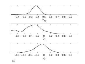
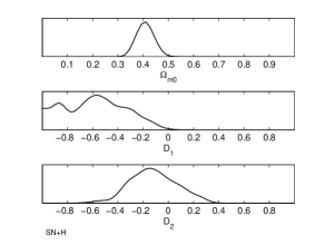
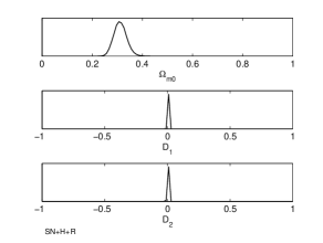
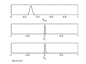
Figure 1: Posterior probability distributions for oscillating DE model parameters.

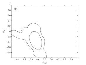
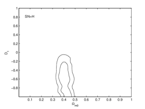
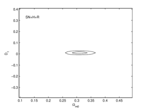
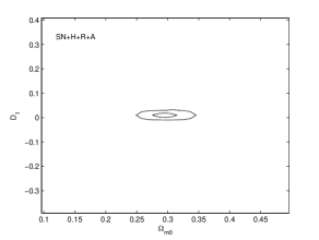
Figure 2: Contour plots representing the $68\%$ and $95\%$ credible interval of the joint posterior probability distribution for $\Omega_{m,0}$ and $D_{1}$ oscillating DE model parameters.

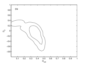
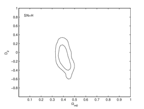
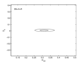
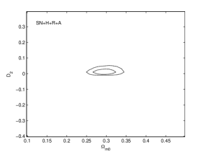
Figure 3: Contour plots representing the $68\%$ and $95\%$ credible interval of the joint posterior probability distribution for $\Omega_{m,0}$ and $D_{2}$ oscillating DE model parameters.

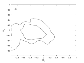
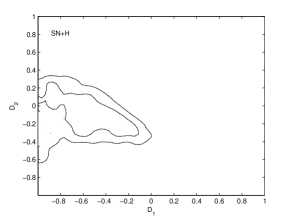
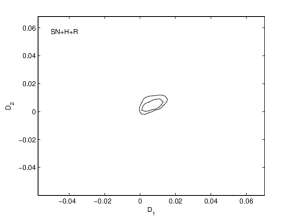
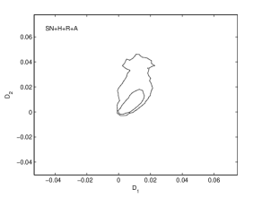
Figure 4: Contour plots representing the $68\%$ and $95\%$ credible interval of the joint posterior probability distribution for $D_{1}$ and $D_{2}$ oscillating DE model parameters.

As one can see after inclusion all data to the analysis we obtain the values for $D_{1}$ and $D_{2}$ parameters which are close to zero. Due to that we also consider two models which are special cases of the oscillating dark energy model:

1. Osc DE 1: $C_{2}=0\Rightarrow w_{X}(z)=-1+C_{1}(1+z)^{3}\cos(\ln(1+z))$,
   $H(z)=H_{0}\sqrt{\Omega_{\Lambda,0}\exp(-0.9C_{1})\exp{\bigg{(}0.3C_{1}(1+z)^{3}\Big{[}3\cos(\ln(1+z))+\sin(\ln(1+z))\Big{]}\bigg{)}}+\Omega_{m,0}(1+z)^{3}+\Omega_{r,0}(1+z)^{4}}$, where $\Omega_{r,0}\simeq 0.5*10^{-4}$ and $\Omega_{\Lambda,0}=1-\Omega_{m,0}-\Omega_{r,0}$.

2. Osc DE 2: $C_{1}=0\Rightarrow w_{X}(z)=-1+C_{2}(1+z)^{3}\sin(\ln(1+z))$,
   $H(z)=H_{0}\sqrt{\Omega_{\Lambda,0}\exp(0.3C_{2})\exp{\bigg{(}-0.3C_{2}(1+z)^{3}\Big{[}\cos(\ln(1+z))-3\sin(\ln(1+z))\Big{]}\bigg{)}}+\Omega_{m,0}(1+z)^{3}+\Omega_{r,0}(1+z)^{4}}$, where $\Omega_{r,0}\simeq 0.5*10^{-4}$ and $\Omega_{\Lambda,0}=1-\Omega_{m,0}-\Omega_{r,0}$

To constrain values of parameters for models defined above we repeat the calculation described before. Results are gathered in Table 2 and 3 respectively. Posterior probabilities are presented on Figure 5 and 7 respectively. Two dimensional contour plots in the ($\Omega_{m,0}$, $C_{i}$) plane are presented on Figure 6 and 8 respectively.

	SN				SN+H
	Best fit	Mean	$68\%$	$95\%$	Best fit	Mean	$68\%$	$95\%$
$\Omega_{m,0}$	$0.36$	$0.37$	$<0.30,0.44>$	$<0.20,0.48>$	$0.40$	$0.40$	$<0.36,0.45>$	$<0.19,0.48>$
$C_{1}$	$-0.19$	$-0.33$	$<-0.55,-0.07>$	$<-0.92,0.07>$	$-0.34$	$-0.42$	$<-0.70,-0.18>$	$<-0.95,0.11>$
$\chi^{2}$	$194.99$				$206.75$
	SN+H+R				SN+H+R+A
	Best fit	Mean	$68\%$	$95\%$	Best fit	Mean	$68\%$	$95\%$
$\Omega_{m,0}$	$0.31$	$0.32$	$<0.29,0.34>$	$<0.27,0.38>$	$0.29$	$0.29$	$<0.27,0.31>$	$<0.26,0.32>$
$C_{1}$	$0.97*10^{-6}$	$0.14*10^{-4}$	$<0.66*10^{-6},$	$<0.17*10^{-6},$	$0.42*10^{-6}$	$0.79*10^{-6}$	$<0.40*10^{-6},$	$<0.31*10^{-7},$
			$0.22*10^{-4}>$	$0.71*10^{-4}>$			$0.12*10^{-5}>$	$0.14*10^{-5}>$
$\chi^{2}$	$211.03$				$211.94$

Table 2: Values for oscillating DE 1 model parameters obtained via $\chi^{2}$ minimization (best fit), values of the mean with the $68\%$ and $95\%$ credible intervals obtained from the posterior probability distribution for considered Osc DE 1 model parameter.

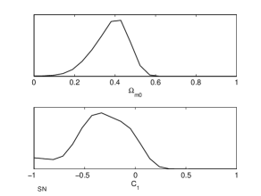
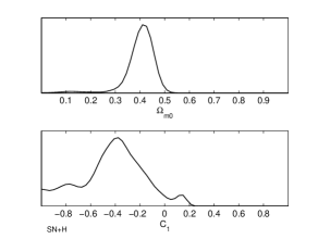
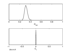
Figure 5: Posterior probability distributions for Osc DE 1 model parameters.

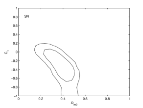
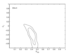
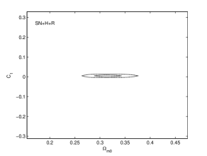
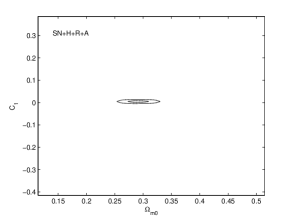
Figure 6: Contour plots representing the $68\%$ and $95\%$ credible interval of the joint posterior probability distribution for $\Omega_{m,0}$ and $C_{1}$ Osc DE 1 model parameters.

	SN				SN+H
	Best fit	Mean	$68\%$	$95\%$	Best fit	Mean	$68\%$	$95\%$
$\Omega_{m,0}$	$0.20$	$0.25$	$<0.22,0.28>$	$<0.20,0.29>$	$0.25$	$0.28$	$<0.26,0.30>$	$<0.24,0.31>$
$C_{2}$	$0.24$	$0.35$	$<0.11,0.54>$	$<-0.03,0.71>$	$0.13$	$0.19$	$<0.14,0.25>$	$<0.12,0.27>$
$\chi^{2}$	$194.37$				$207.65$
	SN+H+R				SN+H+R+A
	Best fit	Mean	$68\%$	$95\%$	Best fit	Mean	$68\%$	$95\%$
$\Omega_{m,0}$	$0.31$	$0.29$	$<0.26,0.31>$	$<0.24,0.34>$	$0.29$	$0.28$	$<0.26,0.30>$	$<0.25,0.32>$
$C_{2}$	$-0.13*10^{-5}$	$0.82*10^{-5}$	$<-0.40*10^{-5},$	$<-0.85*10^{-5},$	$-0.92*10^{-6}$	$0.25*10^{-6}$	$<-0.11*10^{-5},$	$<-0.23*10^{-5},$
			$0.24*10^{-4}>$	$0.32*10^{-4}>$			$0.17*10^{-5}>$	$0.29*10^{-5}>$
$\chi^{2}$	$211.03$				$211.94$

Table 3: Values for oscillating DE 2 model parameters obtained via $\chi^{2}$ minimization (best fit), values of the mean with the $68\%$ and $95\%$ credible intervals obtained from the posterior probability distribution for considered Osc DE 2 model parameter.

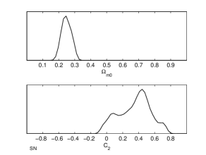
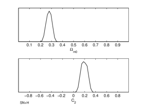
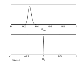
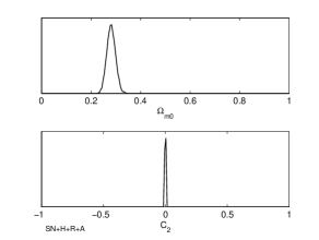
Figure 7: Posterior probability distributions for Osc DE 2 model parameters.

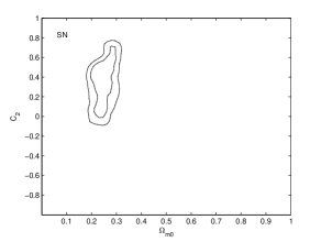
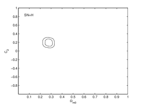
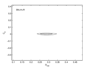
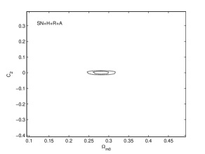
Figure 8: Contour plots representing the $68\%$ and $95\%$ credible interval of the joint posterior probability distribution for $\Omega_{m,0}$ and $C_{2}$ Osc DE 2 model parameters.

The $w_{X}(z)$, $\frac{\rho_{\Lambda}}{\rho_{\Lambda,0}}$ and $\frac{\rho_{\Lambda}}{\rho_{m}}$ functions together with $68\%$ credible interval for considered models ( calculated for the mean of the posterior distributions for the model parameters which are gathered in Table 1, 2, 3 in the SN+H+R+A case) are presented on Figure 9, 10, 11 respectively.

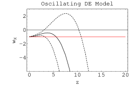
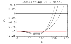
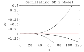
Figure 9: $w_{X}(z)$ for the Osc DE, Osc DE 1, Osc DE 2 Model (black line) together with $68\%$ credible intervals (dashed lines) (calculated for the mean and $68\%$ credible interval of the posterior distributions for the model parameters) and for the $\Lambda$CDM model (red line).

Figure 10: $\frac{\rho_{\Lambda}}{\rho_{\Lambda,0}}$ for the Osc DE, Osc DE 1, Osc DE 2 Model (black line) together with $68\%$ credible intervals (dashed lines) (calculated for the mean and $68\%$ credible interval of the posterior distributions for the model parameters).

Figure 11: $\frac{\rho_{\Lambda}}{\rho_{m}}$ for the Osc DE, Osc DE 1, Osc DE 2 Model (black line) together with $68\%$ credible intervals (dashed lines) (calculated for the mean and $68\%$ credible interval of the posterior distributions for the model parameters).

Finally we made a comparison of Oscillating DE Models, $\Lambda$CDM model and model with linear in scale factor parametrisation of $w$: $w(a)=w_{0}+w_{1}(1-a)$. Analysis was made in the Bayesian framework. Here the best model is this one which has the largest value of the posterior probability. It is convenient to use the posterior odds in analysis, which in the case when no model is favoured a priori is reduced to so called Bayes Factor $B_{ij}$ (the ratio of the evidence for models indexed by $i$ and $j$) Kass and Raftery (1995); Szydlowski et al. (2006). This quantity can be interpreted as a strength of evidence against worse model with respect to the better one: $0\leq|2\ln B_{ij}|<2$–not worth more than a bare mention, $2\leq|2\ln B_{ij}|<6$ – positive, $6\leq|2\ln B_{ij}|<10$ – strong, and $|2\ln B_{ij}|\geq 10$ – very strong. Here we used $BIC$ quantity Schwarz (1978) as an approximation to the minus twice logarithm of the evidence, which is defined in the following way:

$$BIC=-2\ln\mathcal{L}+d\ln N,$$

where $\mathcal{L}$ is the maximum of the likelihood function, $d$ is the number of model parameter and $N$ is the number of data. Values of Bayes Factor (calculated with respect to $\Lambda$CDM model) are gathered in Table 4.

Model	$2\ln B$
$\Lambda$CDM	$0$
Osc DE	$8.75$
Osc DE 1	$3.37$
Osc DE 2	$3.37$
Linear parametrisation	$5.76$

Table 4: Twice logarithm of the Bayes Factor

As one can conclude $\Lambda$CDM model is the best one from the set of models considered in this paper. Evidence in favour this model is strong when comparing with the Osc DE model and positive in the other cases. There is positive evidence in favour model with Linear parametrisation over the Osc DE model. Bayes Factor computed for Osc DE 1 and Osc DE 2 models is close to $1$ which indicate that the information coming from the data (used in analysis) are not enough to favour one of this model over another. In this situation calculation the Bayesian evidence by numerical integration could give better results. Finally Osc DE 1 and Osc DE 2 are favoured over the Osc DE Model and over model with linear in $a$ parametrisation of $w$.

IV Conclusions

In this paper we have placed constraints on a parametrised dark energy model Hrycyna and Szydlowski (2007) using the SNIa data sets, observational H(z) data, the size of the baryonic acoustic oscillation peak from SDSS and the shift parameter from the CMB observations. We study possibility that phantom dark energy is oscillating rather than decaying to $\Lambda$. Such a scenario opens the possibility of the non-minimal coupling to gravity for phantom scalar field. Combining four data bases (SNIa, H(z), CMB, SDSS) we obtain constraints on the oscillating dark energy model parameters $(\Omega_{m},D_{1},D_{2})$ and compare this model with $\Lambda$CDM model and with model with linear in $a$ parametrisation of $w$ in the Bayesian framework. It is found that special cases of oscillating phantom dark energy model ( called Osc DE 1 and Osc DE 2 in this paper) are favoured over the model with linear in $a$ parametrisation of $w$. Cosmological constant case still remains as the best one from the set of considered models.