Transport through single-level quantum dot in a magnetic field

Abstract

We study the effect of an external magnetic field on the transport properties of a quantum dot using a recently developed extension of the functional renormalization group approach to non-equilibrium situations. We discuss in particular the interplay and competition of the different energy scales of the dot and the magnetic field on the stationary non-equilibrium current and conductance. As rather interesting behavior we find a switching behavior of the magnetic field for intermediate correlations and bias voltage.

I Introduction

The investigation of transport through mesoscopic systems has developed into a very active research field in condensed matter during the past decade due to their possible relevance for next-generation electronic devices and quantum computing.goldhaber:2003 ; zutic:2004 The advance in preparation and nano-structuring of layered semiconductorsKouwenhoven et al. (2001) or the handling of molecules respectively nano-tubes has lead to an increasing amount of experimental knowledge about such systems.gershenson:2006

The simplest realization of a mesoscopic system is the quantum dot.Kastner (1992); Kouwenhoven et al. (1997, 2001) It can be viewed as artificial atom coupled to an external bath, whose properties can be precisely manipulated over a wide range.Kouwenhoven et al. (2001) The transport properties of quantum dots in the linear response regime are very well understood from the experimental as well as theoretical point of view.Kouwenhoven et al. (2001) On the other hand, a reliable theoretical description of even the stationary transport in non-equilibrium is still a considerable challenge.

In the present work we study the influence of an external magnetic field $B$ on the stationary transport properties of a single-level quantum dot subject to a bias voltage $V_{B}$ at $T=0$. Quantum dots in external magnetic field have been the subject of interest for some time and experimental studies of these systems have been performed by several groups.De Franceschi et al. (2002); Goldhaber-Gordon et al. (1998); Ralph and Buhrman (1992); Schmid et al. (2000) From a theoretical point of view, non-equilibrium properties in magnetic field were investigated by Meir and Wingreen Meir and Wingreen (1992) combining different methods such as noncrossing approximation (NCA), equations of motion (EOM) and variational wavelenght approach in the limit in which the Coulomb repulsion $U$ is very large. Rosch et al.Rosch et al. (2005) used a perturbative renormalization group, which permits the description of the transport properties in single-level quantum dots for large bias and magnetic fields. König et al.Koenig et al. (1996) studied tunneling through a single-level quantum dot in the presence of strong Coulomb repulsion beyond the perturbative regime by means of a real-time diagrammatic formulation. However, a theory that allows to access intermediate coupling, bias voltage and magnetic field strenghts on a unique footing is missing so far.

Here, we use as theoretical approach the functional renormalization group (fRG)Salmhofer (1998) extended to non-equilibrium, which we have introduced in a recent publication.Gezzi et al. (2007) We discuss how the current $J$ and the differential conductance $G$ are affected by $B$ and by the competition between magnetic field and bias voltage. We show in particular that $B$ is responsible for a switching behaviour in $J$ as function of $V_{B}.$ Interesting are also the individual contributions of spin up and down electrons, split by the presence of the magnetic field, to the transport parameters. To test our non-equilibrium fRG we have moreover studied, as limiting case, the equilibrium situation $V_{B}=0$, in order to compare the results of the imaginary-time fRG, which has been shown to provide a very good description of transport through mesoscopic systems in the linear response regime.Karrasch et al. (2006)

The paper is organized as follows: The next section is dedicated to a brief description of the model we use, namely the single impurity Anderson model (SIAM). Based on the derivation in Gezzi et al. (2007) we will provide an expression for the non-equilibrium fRG equations studied in this work. In Sec. III we present our results for the stationary transport properties. The limit $V_{B}\to 0$ is investigated first to make contact to previous work and find the regime, where our method is applicable. We then discuss how the transport parameters current $J$ and conductance $G$ behave as functions of an applied bias-voltage with and without magnetic field. Finally we consider the range of applicability of the non-equilibrium fRG in the presence of $B$. A summary and conclusions will finish the paper.

II Flow equations for single-level quantum dot in magnetic field

We consider in the following a quantum dot consisting of a single level $\varepsilon_{\sigma}$ with spin quantum number $\sigma=\pm 1$, coupled to left ($L$) and right ($R$) leads. The electronic states in the leads are described by a continuum of single-particle levels with dispersion $\varepsilon_{\vec{k}\sigma\alpha}$, where $\vec{k}$ denotes the wave vector and $\alpha=L$, $R$. Furthermore, we assume that the leads are always in equilibrium. The dot and the leads are coupled through an energy and spin independent hybridization $V_{\alpha}$. Finally, if two electrons occupy the dot, they experience a Coulomb repulsion $U$. This situation is described by the long-known single impurity Anderson model, given by the HamiltonianAnderson (1961)

$$H = \sum_{\vec{k}\sigma\alpha}\varepsilon_{\vec{k}\sigma\alpha}c^{\dagger}_{\vec{k}\sigma\alpha}c^{\phantom{{\dagger}}}_{\vec{k}\sigma\alpha}$$ (1)

$$+\sum_{\sigma}\varepsilon_{\sigma}d^{\dagger}_{\sigma}d^{\phantom{{\dagger}}}_{\sigma}+U\left(n_{\uparrow}-\frac{1}{2}\right)\left(n_{\downarrow}-\frac{1}{2}\right)$$

$$+\frac{1}{\sqrt{N}}\sum_{\vec{k}\sigma\alpha}\left[V_{\alpha}c^{\dagger}_{\vec{k}\sigma\alpha}d^{\phantom{{\dagger}}}_{\sigma}+h.c.\right]\;.$$

The left and right reservoirs can have different chemical potentials $\mu_{\alpha}$ through an applied bias voltage $V_{B}=\mu_{L}-\mu_{R}$. An external magnetic field is taken into account by the Zeeman splitting of the dot level, i.e. $\varepsilon_{\sigma}=V_{G}\pm\sigma B/2$, where we introduced the gate voltage $V_{G}$, which controls the filling on the dot. Since the magnetic fields applied are much smaller than the Fermi energy of the leads, its effect on the electrons in the leads can be ignored for the present purpose.

The detailed derivation of the fRG flow equations in a general non-equilibrium situation has been already discussed in Ref. Gezzi et al., 2007. Since one obtains an infinite hierarchy of differential equations for the irreducible $n$-particle vertices depending on a cutoff parameter $\Lambda$ in this approach,Salmhofer and Honerkamp (2001); Hedden et al. (2004); Gezzi et al. (2007) a truncation is necessary for actual calculations, which we realize by setting the three-particle vertex $\gamma_{3}^{\Lambda}\equiv 0$. In addition to this truncation of the hierarchy of differential equations, we further neglect the energy dependence of the vertex function $\gamma_{2}^{\Lambda}\equiv\gamma^{\Lambda}$, which results in an energy independent single particle self-energy $\Sigma^{\Lambda}$. Note that in the non-equilibrium approach, all quantities become tensors with respect to the branches $+$ and $-$ of the Keldysh contour.Keldysh (1965); Gezzi et al. (2007) In particular the Green function and self-energy are matrices, which we denote by $\hat{G}$ and $\hat{\Sigma}$, respectively.

Last but not least, we have to specify how the cutoff $\Lambda$ is introduced. As usualHedden et al. (2004) we choose a $\Theta$-cutoff on the level of the non-interacting dot here, i.e.

$$\hat{G}_{d\sigma,0}^{\Lambda}(\omega)=\Theta(\Lambda-|\omega|)\hat{G}_{d\sigma,0}$$

with $\hat{G}_{d\sigma,0}(\omega)$ the Green function matrix of the dot for $U=0$. Since in this case we have to deal with a non-interacting system, the corresponding expressions can be derived straightforwardly. For simplicity we assume that the dispersions $\varepsilon_{\vec{k}\sigma\alpha}$ and hybridizations $V_{\alpha}$ are identical for $\alpha=L$ and $\alpha=R$. In that case the coupling between dot and leads is characterized by the quantities

$$\Gamma_{\alpha}=\pi|V|^{2}N_{\rm F}\equiv\frac{\Gamma}{2}\;\;,$$ (2)

with $N_{\rm F}$ the local density of states of the leads at the dot site. The result for $\hat{G}_{d\sigma,0}(\omega)$ then reads Gezzi et al. (2007):

$$G_{d\sigma,0}^{--}(\omega) = \frac{\omega-\varepsilon_{\sigma}-i\Gamma\left[1-f_{L}(\omega)-f_{R}(\omega)\right]}{(\omega-\varepsilon_{\sigma})^{2}+\Gamma^{2}}\;,$$ (3)

$$G_{d\sigma,0}^{++}(\omega) = -[G_{d\sigma,0}^{--}(\omega)]^{*}\;,$$ (4)

$$G_{d\sigma,0}^{-+}(\omega) = i\frac{\Gamma\left[f_{L}(\omega)+f_{R}(\omega)\right]}{(\omega-\varepsilon_{\sigma})^{2}+\Gamma^{2}}\;,$$ (5)

$$G_{d\sigma,0}^{+-}(\omega) = -i\frac{\Gamma\left[f_{L}(-\omega)+f_{R}(-\omega)\right]}{(\omega-\varepsilon_{\sigma})^{2}+\Gamma^{2}}\;,$$ (6)

where $f_{\alpha}(\pm\omega):=f\left(\pm(\omega-\mu_{\alpha})\right)$ are the Fermi functions of the leads.

With these definitions and approximations, the resulting system of differential equations for the spin-dependent single particle self-energy and two-particle vertex we are going to integrate is given by (for details see e.g. App. B in Ref. Gezzi et al., 2007)

$$\frac{d}{d\Lambda}\Sigma^{\alpha\beta,\Lambda}_{\sigma}=-\frac{1}{2\pi}\sum\limits_{\sigma^{\prime}}\sum\limits_{\omega=\pm\Lambda}\sum\limits_{\mu\nu}\tilde{G}^{\mu\nu,\Lambda}_{\sigma^{\prime}}(\omega)\gamma^{\alpha\nu\beta\mu,\Lambda}_{\sigma,\sigma^{\prime},\sigma,\sigma^{\prime}}\;,$$ (7)

$$\frac{d}{d\Lambda}\gamma^{\alpha\beta\gamma\delta,\Lambda}_{\sigma_{1}^{\prime},\sigma_{2}^{\prime};\sigma_{1},\sigma_{2}}=\frac{1}{4\pi}\sum_{\omega=\pm\Lambda}\sum_{\sigma_{3},\sigma_{4}}\sum_{\mu,\nu\rho,\eta}\bigg{(} \!\!\!\tilde{G}^{\rho\eta,\Lambda}_{\sigma_{3}}(-\omega)\tilde{G}^{\nu\mu,\Lambda}_{\sigma_{4}}(\omega) \!\!\!\gamma^{\alpha\beta\rho\nu,\Lambda}_{\sigma_{1}^{\prime},\sigma_{2}^{\prime};\sigma_{3},\sigma_{4}}\gamma^{\eta\mu\gamma\delta,\Lambda}_{\sigma_{3},\sigma_{4};\sigma_{1},\sigma_{2}}-$$ (8)

$$\!\!\!\tilde{G}^{\eta\rho,\Lambda}_{\sigma_{3}}(\omega)\tilde{G}^{\nu\mu,\Lambda}_{\sigma_{4}}(\omega)\Big{[} \!\!\!\gamma^{\alpha\mu\gamma\eta,\Lambda}_{\sigma_{1}^{\prime},\sigma_{4};\sigma_{1},\sigma_{3}}\gamma^{\rho\beta\nu\delta,\Lambda}_{\sigma_{3},\sigma_{2}^{\prime};\sigma_{4},\sigma_{2}}+\gamma^{\alpha\rho\gamma\nu,\Lambda}_{\sigma_{1}^{\prime},\sigma_{3};\sigma_{1},\sigma_{4}}\gamma^{\mu\beta\eta\delta,\Lambda}_{\sigma_{4},\sigma_{2}^{\prime};\sigma_{3},\sigma_{2}}-$$

$$\!\!\!\gamma^{\beta\mu\gamma\eta,\Lambda}_{\sigma_{2}^{\prime},\sigma_{4};\sigma_{1},\sigma_{3}}\gamma^{\rho\alpha\nu\delta,\Lambda}_{\sigma_{3},\sigma_{1}^{\prime};\sigma_{4},\sigma_{2}}-\gamma^{\beta\rho\gamma\nu,\Lambda}_{\sigma_{2}^{\prime},\sigma_{3};\sigma_{1},\sigma_{4}}\gamma^{\mu\alpha\eta\delta,\Lambda}_{\sigma_{4},\sigma_{1}^{\prime};\sigma_{3},\sigma_{2}}\Big{]}\bigg{)}\;\;.$$

In expressions (7) and (8)

$$\tilde{G}_{\sigma}^{\mu\nu,\Lambda}(\omega)=\left[\frac{1}{\hat{G}_{d\sigma,0}(\omega)^{-1}-\hat{\Sigma}_{\sigma}^{\Lambda}}\right]^{\mu\nu}\;\;,$$

and the upper small greek indices refer to the branches of the Keldysh contour. The initial conditions at $\Lambda=\infty$ are are given by

$$\Sigma_{\sigma}^{\Lambda=\infty}=0$$

and

$$\gamma_{\sigma_{1}^{\prime},\sigma_{2}^{\prime};\sigma_{1},\sigma_{2}}^{\alpha\alpha\alpha\alpha,\Lambda=\infty}=i\alpha U(\delta_{\sigma_{1},\sigma_{1}^{\prime}}\delta_{\sigma_{2},\sigma_{2}^{\prime}}-\delta_{\sigma_{1},\sigma_{2}^{\prime}}\delta_{\sigma_{2},\sigma_{1}^{\prime}})\;\;.$$

All other components of $\gamma^{\Lambda=\infty}=0$. The integration of the equations (7) and (8) has to be done until $\Lambda=0$ is reached.

Compared to the system obtained in Ref. Gezzi et al., 2007 without external magnetic field the set of eqs. (7) and (8) show a more complicated structure which manifests itself in a spin-dependent flow for the selfenergy and the vertex. As $V_{B}\to 0,$ it can be shown Karrasch et al. (2006) that the vertex $\gamma_{2}$ can be parametrized as

$$\gamma^{\alpha\beta\gamma\delta,\Lambda}_{\sigma_{1}^{\prime},\sigma_{2}^{\prime};\sigma_{1},\sigma_{2}}=\delta_{\sigma_{1}^{\prime},\sigma_{1}}\delta_{\sigma_{2}^{\prime},\sigma_{2}}U^{\alpha\beta\gamma\delta,\Lambda}-\delta_{\sigma_{2}^{\prime},\sigma_{1}}\delta_{\sigma_{1}^{\prime},\sigma_{2}}U^{\beta\alpha\gamma\delta,\Lambda},$$

with spin-independent interaction parameters $U$. It is thus tempting to use the same parametrization out of equilibrium, too, resulting in the simpler set of equations

$$\frac{d}{d\Lambda}\Sigma^{\alpha\beta,\Lambda}_{\sigma}=-\frac{1}{2\pi}\sum\limits_{\omega=\pm\Lambda,\gamma,\delta}\left[\left(\tilde{G}_{\sigma}^{\gamma\delta,\Lambda}(\omega)+\tilde{G}_{-\sigma}^{\gamma\delta,\Lambda}(\omega)\right)U^{\alpha\beta\gamma\delta,\Lambda}-\tilde{G}_{\sigma}^{\gamma\delta,\Lambda}(\omega)U^{\beta\alpha\gamma\delta,\Lambda}\right]\;\;,$$ (9)

$$\frac{d}{d\Lambda}U^{\alpha\beta\gamma\delta,\Lambda}=\frac{1}{4\pi}\sum_{\omega=\pm\Lambda}\sum_{\mu,\nu\rho,\eta}\biggr{(}\tilde{G}^{\rho\eta,\Lambda}_{-\sigma}(-\omega)\tilde{G}^{\nu\mu,\Lambda}_{\sigma}(\omega)U^{\alpha\beta\eta\nu,\Lambda}U^{\rho\mu\gamma\delta,\Lambda}+\tilde{G}^{\rho\eta,\Lambda}_{\sigma}(-\omega)\tilde{G}^{\nu\mu,\Lambda}_{-\sigma}(\omega)U^{\beta\alpha\eta\nu,\Lambda}U^{\mu\rho\gamma\delta,\Lambda}-$$

$$\left[\tilde{G}^{\eta\rho,\Lambda}_{\sigma}(\omega)\tilde{G}^{\nu\mu,\Lambda}_{\sigma}(\omega)+\tilde{G}^{\eta\rho,\Lambda}_{-\sigma}(\omega)\tilde{G}^{\nu\mu,\Lambda}_{-\sigma}(\omega)\right]U^{\alpha\mu\gamma\eta,\Lambda}U^{\rho\beta\nu\delta,\Lambda}-\tilde{G}^{\eta\rho,\Lambda}_{\sigma}(\omega)\tilde{G}^{\nu\mu,\Lambda}_{\sigma}(\omega)U^{\alpha\mu\gamma\eta,\Lambda}U^{\beta\rho\nu\delta,\Lambda}-$$

$$\tilde{G}^{\eta\rho,\Lambda}_{-\sigma}(\omega)\tilde{G}^{\nu\mu,\Lambda}_{-\sigma}(\omega)U^{\mu\alpha\gamma\eta,\Lambda}U^{\rho\beta\nu\delta,\Lambda}+\left[\tilde{G}^{\eta\rho,\Lambda}_{\sigma}(\omega)\tilde{G}^{\nu\mu,\Lambda}_{\sigma}(\omega)+\tilde{G}^{\eta\rho,\Lambda}_{-\sigma}(\omega)\tilde{G}^{\nu\mu,\Lambda}_{-\sigma}(\omega)\right]U^{\alpha\rho\gamma\nu,\Lambda}U^{\mu\beta\eta\delta,\Lambda}-$$

$$\tilde{G}^{\eta\rho,\Lambda}_{\sigma}(\omega)\tilde{G}^{\nu\mu,\Lambda}_{\sigma}(\omega)U^{\alpha\rho\gamma\nu,\Lambda}U^{\beta\mu\eta\delta,\Lambda}-\tilde{G}^{\eta\rho,\Lambda}_{-\sigma}(\omega)\tilde{G}^{\nu\mu,\Lambda}_{-\sigma}(\omega)U^{\rho\alpha\gamma\nu,\Lambda}U^{\mu\beta\eta\delta,\Lambda}-$$

$$\tilde{G}^{\eta\rho,\Lambda}_{\sigma}(\omega)\tilde{G}^{\nu\mu,\Lambda}_{-\sigma}(\omega)U^{\mu\beta\gamma\eta,\Lambda}U^{\alpha\rho\nu\delta,\Lambda}+\tilde{G}^{\eta\rho,\Lambda}_{-\sigma}(\omega)\tilde{G}^{\nu\mu,\Lambda}_{\sigma}(\omega)U^{\rho\beta\gamma\nu,\Lambda}U^{\alpha\mu\eta\delta,\Lambda}\bigg{)}\;\;.~{}$$ (10)

By investigating the structure of the vertex for the full spin-dependent flow at $\Lambda=0$ it turns out, however, that the parametrized version breaks exact symmetries for exchanging indices. Due to the significantly reduced numerical effort for integrating Eqs. (9) and (10), it remains interesting to examine its value as an approximation.

After integration of system (7), (8) or (9), (10) we insert the resulting selfenergy into the Meir-Wingreen formula for the currentMeir and Wingreen (1992); Gezzi et al. (2007)

$$J_{\sigma}=\frac{ie\Gamma}{2\pi\hbar}\int d\epsilon\left[f_{L}(\epsilon)-f_{R}(\epsilon)\right]\left(\tilde{G}^{+-}_{d\sigma}(\epsilon)-\tilde{G}^{-+}_{d\sigma}(\epsilon)\right),$$ (11)

where $\hat{G}_{d\sigma}$ denotes the full spin dependent one-particle impurity Green function.

The conductance finally is obtained from (11) by numerical differentiation with respect to $V_{B}$.

III Results

Together with the initial conditions for self-energy and two-particle vertex we can now integrate the differential equations using a standard Runge-Kutta solver. Although the systems of equations are valid for $T>0$, too, we restrict our discussion to the case $T=0$ for simplicity, noting that preliminary results for $T>0$ in the weak-coupling regime are in agreement with previous studies and, in the linear response regime, NRG results.

III.1 Test of the parametrized flow

Let us start by comparing the full flow according to Eqs. (7) and (8) with the parametrized ones Eqs. (9) and (10). We observe a good agreement at small $V_{B}$ for $\Sigma^{-+,\Lambda}$ (see Fig. 1b),

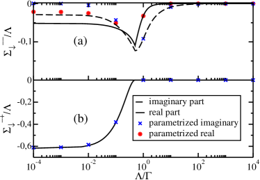
Figure 1: (color online) (a) Flow of real (full curve and stars) and imaginary part (dashed curve and crosses) of $\Sigma^{--,\Lambda}_{\downarrow}/\Gamma,$ for $V_{G}/\Gamma=0,$ $U/\Gamma=5,$ $V_{B}/\Gamma=1,$ $B/\Gamma=0.116$. The continuous lines represent the solutions of Eqs. (7) and (8), the symbols the parametrized version Eqs. (9) and (10). (b) Flow of $\Sigma^{-+,\Lambda}_{\downarrow}/\Gamma$.

while deviations appear in $\Sigma^{--,\Lambda}$ (see Fig. 1a). However, since $|\Sigma^{-+,\Lambda}|\gg|\Sigma^{--,\Lambda}|$, this does not affect the behaviour of experimentally relevant quantities even for larger $B$, as can be seen for the case of the conductance $G$ as function of gate voltage in Fig. 2.

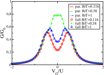
Figure 2: (color online) Conductance $G$ normalized to $G_{0}=2e^{2}/h$ as function of $V_{G}$ for $U/\Gamma=5,$ $V_{B}/\Gamma=1$ and several values of $B$.

Increasing the bias voltage, the agreement is still good for small $B$ (see Fig. 3, full curve and circles). As soon as we increase the magnetic field, $\mathrm{Im\,}\Sigma^{-+,\Lambda}$, too, shows deviations between the

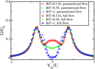
Figure 3: (color online) The same parameters as in Fig. 2 except for $V_{B}/\Gamma=3$.

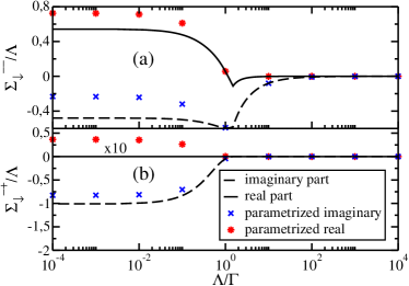
Figure 4: (color online) The same parameters as in Fig. 1 except for $V_{B}/\Gamma=3$ and $B/\Gamma=1.$ In (b) the real part of $\Sigma^{-+}$ has been rescaled by a factor ten to make it visible.

full and parametrized flow (see Fig. 4). In particular, the flow of the parametrized system gives rise to a small real component of $\Sigma^{+-,\Lambda}$ at $\Lambda=0$ (Fig. 4b), which actually should not exist, and leads to unphysical breaking of the particle-hole symmetry in physical quantities like the conductance, as is visible from the dashed and dot-dashed curves in Fig. 3.

We thus can conclude that the parametrized set of flow equations is a reasonable approximation at least for calculating the conductance as long as $V_{B}$ and the magnetic field $B$ become not too large.

III.2 Equilibrium case

Before studying the influence of a magnetic field on stationary non-equilibrium transport at $T=0$, we first present results for the linear response regime, i.e. the limit $V_{B}=\mu_{L}-\mu_{R}\to 0$. This limit can serve as a test for the non-equilibrium fRG, because it should reproduce the imaginary-time fRG results.Karrasch et al. (2006)

In Fig. 5 we compare

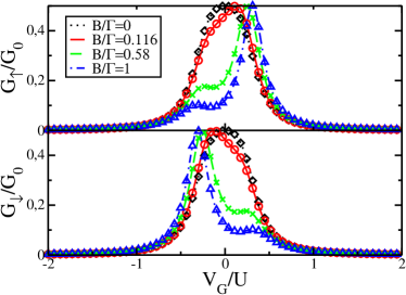
Figure 5: (color online) Conductance $G_{\sigma}$ from the individual spin channels in the limit $V_{B}\to 0$ normalized to $G_{0}=2e^{2}/h$ as function of $V_{G}/U$ for $U/\Gamma=5$ and several values of $B$. Symbols were obtained from the non-equilibrium fRG, lines from the imaginary-time fRG of Karrasch et al. (2006).

the contributions $G_{\sigma}$ to the conductance from the individual spin channels calculated with the non-equilibrium fRG (symbols) as $V_{B}\to 0$ for different values of $B$ to the results of the imaginary-time fRG obtained by Karrasch et al. (2006) (lines). We note, that for $V_{B}/\Gamma=0$ our calculations perfectly reproduce the results of Karrasch et al. (2006). We see that, as soon as the magnetic field increases, $G_{\sigma}$ starts to split into two peaks which reflects the field dependent shifts of the spectral functions for up and down spin.

We would like to mention here that for too large $U$ and magnetic field a crossing of solutions of the differential equations appears, and the numerical procedure picks the one on the wrong Riemannian sheet. At present we do not know how to avoid this numerical instabilty, which limits the applicability of the method to intermediate coupling parameters. We will come back to this problem later.

For an extensive discussion of the linear response results with an applied magnetic field we refer the reader to the seminal paper by Karrasch et al. (2006).

III.3 Non-equilibrium

Switching on the bias voltage $V_{B}$ we observe different behaviours of the conductance $G$ as a function of the gate voltage $V_{G}$ depending on the competition between the voltage and the magnetic field. In Fig. 6a-d we present $G=G_{\uparrow}+G_{\downarrow}$ as function of $V_{G}$ for fixed Coulomb interaction $U/\Gamma=5$ and $V_{B}/\Gamma=0$, $1$, $3$, $5$ for different values of $B$. We observe a drastic change of the conductance due to the interplay of $V_{B}$ and $B$.

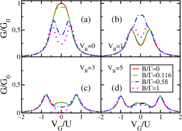
Figure 6: (color online) Total conductance $G$ normalized to $G_{0}=2e^{2}/h$ as function of $V_{G}/U$ for $U/\Gamma=5$, $V_{B}/\Gamma=0$, $1$, $3$, $5$ and several values of $B/\Gamma$.

In particular, we see that for small bias ($V_{B}/\Gamma=1$, Fig. 6b) and fields $B/\Gamma=0.116$, $G$ consists of just two peaks separated by $U$. If we now increase the value of the magnetic field, the conductance at small $V_{G}$ initially strongly increases (dashed and dot-dashed curves in Fig. 6b), the peaks disappear and a small plateau appears. Increasing $B$ further, the plateau disappears and we get back the two peaks separated by a rather deep valley and two shoulders whose spacing is $\Delta\approx U$.

This behaviour can be explained as follows: The spectral density for each spin channel is split by $V_{B}$ into two peaks moving the spectral weight to higher frequencies and decreasing it in the region $V_{G}\approx 0$.Gezzi et al. (2007) Switching on $B$ will lead to a splitting $\sim B$ of each peak, due to field induced shifts of the spectral functions from the individual spin contributions. Thus, increasing $B$, the two outer peaks move away from each other while the inner ones get closer and even merge, enhancing the conductance at $V_{G}\approx 0$. As direct consequence we observe a small plateau for $V_{G}\approx 0$ (see Fig. 6b). Further increasing $B$, these contributions will again drift apart, leading to a collapse of the conductance and disappearance of the plateau.

Completely different is the behaviour for $V_{B}/\Gamma=3$ and $V_{B}/\Gamma=5$ (Fig. 6c and d). We find a monotonic decrease of G with the magnetic field. In addition the field dependence is initially weaker than in Fig. 6b. We interpret this behaviour in the following way: For large $V_{B}$, the Fermi window in e.g. Eq. (11) will lead to an averaging over a large energy region. Thus structures due to the magnetic field at too small energies will be washed out, i.e. the subtle interplay between the rearrangement of spectral weight due to $V_{B}$ and the shifts induced by the magnetic field $B$ cannot be resolved any more.

III.4 Current and Conductance as function of the applied bias

The non-monotonic behaviour of $G(V_{G}=0)$ for moderate $V_{B}$ as function of the external magnetic field $B$ is an interesting feature we want to explore in somewhat more detail in the following. To this end we calculated the current $J$ and the differential conductance $G=dJ/dV_{B},$ at $V_{G}/\Gamma=0$ and $U/\Gamma=5$ as function of the applied bias for different values of $B$. The results are collected in Fig. 7.

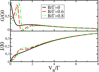
Figure 7: (color online) Total current normalized to $J_{0}=G_{0}\frac{\Gamma}{e}$ and conductance as function of the bias voltage $V_{B}/\Gamma$ for $V_{G}/\Gamma=0$, $U/\Gamma=5$ and several values of $B$.

Compared to the case $B=0$ (full line) we see that a finite magnetic field $B$ basically induces two features. First, as is also the case for $B=0$ at larger $U$, we observe a shoulder in the current, resulting in a small region of negative differential conductance. More interesting, however, is the appearance of an almost unitary conductance peak at $V_{B}\approx B$ for intermediate magnetic fields. For large fields the features is suppressed again. This behaviour can be explained by noting that when $V_{B}\approx B$, the electrochemical potentials $\mu_{L,R}$ of the leads are close to the split dot levels, respectively, therefore the tunnel probability from the leads to the dot is enhanced. For $V_{B}\gg B$ the curves converge again to the same values, i.e. $B$ does not influence the current any longer, the behavior is dominated by the now rather wide Fermi window.

Thus we observe that $B$ can act as a switch, suppressing the current for small $V_{B}$ and leading to a steep increase of the current in the voltage range $V_{B}\approx B$.

III.5 Range of applicability of the fRG

Let us finally discuss in which range of parameters the non-equilibrium fRG furnishes reliable results. In Fig. 8 we show the transport parameters plotted as function of the magnetic field for different bias voltages in the weak ($\frac{U}{\pi\Gamma}<1$, Fig. 8a) and intermediate coupling regime ($\frac{U}{\pi\Gamma}\gtrsim 1$, Fig. 8b). While for $\frac{U}{\pi\Gamma}<1$ the fRG always converged smoothly,

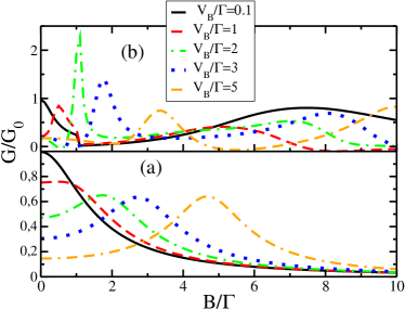
Figure 8: (color online) Total conductance normalized to $G_{0}=2e^{2}/h$ plotted versus $B/\Gamma$ for $V_{G}/\Gamma=0$ and several values of $V_{B}$. (a) weak coupling regime $U/\Gamma=1$. (b) strong coupling regime $U/\Gamma=5$.

we see that for $\frac{U}{\pi\Gamma}>1$ the curves show a discontinuity in $G$ (see Fig. 88b for $V_{B}/\Gamma=1$). Increasing $V_{B}$ further this discontinuity disappears but for $V_{B}/\Gamma=2..3$ the conductance now overshoots the unitary limit in the range $1<B/\Gamma<2$.

While these results are at first sight very disturbing, they can be traced back to a crossing of solutions of the differential equations in this parameter regime. As already mentioned earlier and discussed in detail in Ref. Gezzi et al., 2007, the Runge-Kutta algorithm picks the wrong solution, leading to the observed pathologies in the physical properties. At very large bias $V_{B}\geq U$ the solution of the differential equations does not show this problem any longer.

This means that our approach is due to numerical reasons not reliable in this parameter range and possibly for larger magnetic fields. We are presently not aware of any algorithm that can avoid this numerical difficulty related to the appearance of a pole in the physical Riemannian sheet.

IV Summary and outlook

In this work we applied the non-equilibrium fRG approach to the stationary transport through a single-level quantum dot subject to a constant bias $V_{B}$ and magnetic field $B$ at $T=0$. Besides the truncation of the infinite hierarchy of the fRG differential equations at the two-particle level we also neglected the energy dependence of the two-particle vertex function $\gamma_{2}$, resulting in an energy independent single-particle self energy. Guided by the structure of the fRG equations in equilibrium, we studied as further possible approximation the neglect of the spin-dependence in the vertex function $\gamma_{2}$. This latter approximation further significantly reduces the complexity of the system of differential equations. We compared the results of this approximation with those from the equations maintaining the full spin dependence, finding that for not too large $V_{B}$ and field $B$ it actually can be used to accurately calculate transport properties.

Although the truncation and especially the neglect of the energy dependence must be viewed as rather crude approximations, we have shown that one can obtain reasonable results for the transport parameters $J$ and $G$ up to the intermediate coupling regime for an extended regime of the parameters $V_{B}$ and $B$. A particularly interesting observation is the switching behaviour found in the current for intermediate values of $V_{B}$ and magnetic field $B$, which we could explain with the interplay of the different structures we expect in the single-particle spectra as function of the gate voltage and $B$. We also showed that for bias voltage $V_{B}\to 0$ we recover, as expected, the linear response results by Karrasch et al. (2006).

As an important future step we view the introduction of the energy dependence in the flow equations of the non-equilibrium fRG. Besides curing certain deficiencies not discussed here (see Gezzi et al. (2007)), we expect that this step will extend the range of applicability of our formalism to larger magnetic fields and Coulomb interaction. Furthermore, coping with the full energy dependence of the vertex will eventually enable us to study time-dependent phenomena off equilibrium, which will open a wide and interesting field of physical phenomena and applications.

- (1) I. Žutić, J. Fabian, and S. Das Sarma, Rev. Mod. Phys. 76, 323 (2004).
- (2) D. Goldhaber-Gordon, and I. Goldhaber-Gordon, Nature 412, 594 (2001).
- Kouwenhoven et al. (2001) L. P. Kouwenhoven, D. G. Austing, and S. Tarucha, Rep. Prog. Phys. 64, 701 (2001).
- (4) M.E. Gershenson, V. Podzorov, and A.F. Morpurgo, Rev. Mod. Phys. 78, 973 (2006).
- Kastner (1992) M. A. Kastner, Rev. Mod. Phys. 64, 849 (1992).
- Kouwenhoven et al. (1997) L. P. Kouwenhoven et al., in Mesoscopic Electron Transport, edited by L. L. Sohn et al. (Dordrecht: Kluwer, 1997), p. 105.
- Ralph and Buhrman (1992) D.C. Ralph and R.A Buhrman, Phys. Rev. Lett. 69, 2118 (1992).
- Schmid et al. (2000) J. Schmid J. Weis K. Eberl and K. v.Klitzing, Phys. Rev. Lett. 84, 5824 (2000).
- Goldhaber-Gordon et al. (1998) H. Shtrikman, D. Mahalu, and D. Abusch-Magder, U. Meirav,and M.A. Kastner Nature 391, 156 (1998).
- De Franceschi et al. (2002) S. De Franceschi, W.G van der Wiel, J.L Elzermann, J.J Wijpkema, T. Fujisawa, S Tarucha,and L.P. Kouwenhoven, Phys. Rev. Lett 89, 156801 (2002).
- Meir and Wingreen (1992) Y. Meir and N. S. Wingreen, Phys. Rev. Lett. 69, 2118 (1992).
- Rosch et al. (2005) A. Rosch, J. Paaske, J. Kroha, and P. Wölfle, J. Phys. Soc. Jpn. 74, 118 (2005).
- Koenig et al. (1996) J. Koenig, J. Schmid, and H. Schoeller, G. Schoen, Phys. Rev. B 54, 16820 (1996).
- Salmhofer (1998) M. Salmhofer, Renormalization (Springer, Berlin, 1998).
- Gezzi et al. (2007) R. Gezzi, T. Pruschke, and V. Meden, Phys. Rev. B 75, 045324 (2007).
- Karrasch et al. (2006) C. Karrasch, T. Enss, and V. Meden, Phys. Rev. B 73, 235337 (2006).
- Anderson (1961) P. W. Anderson, Phys. Rev. 124, 41 (1961).
- Salmhofer and Honerkamp (2001) M. Salmhofer and C. Honerkamp, Prog. Theor. Phys. 105, 1 (2001).
- Hedden et al. (2004) R. Hedden, V. Meden, T. Pruschke, and K. Schönhammer, J. Phys.: Condens. Matter 16, 5279 (2004).
- Keldysh (1965) L. P. Keldysh, JETP 20, 1018 (1965).
- Meir and Wingreen (1992) Y. Meir and N. S. Wingreen, Phys. Rev. Lett. 68, 2512 (1992).