Magnetic phases in the correlated Kondo-lattice model

Abstract

We study magnetic ordering of an extended Kondo-lattice model including an additional on-site Coulomb interaction between the itinerant states. The model is solved in the dynamical mean-field theory using Wilson’s numerical renormalization group approach as impurity solver. For a bipartite lattice we find at half filling the expected antiferromagnetic phase. Upon doping this phase is gradually suppressed and hints towards phase separation are observed. For large doping the model exhibits ferromagnetism, the appearance of which can at first sight be explained by Rudermann-Kittel-Kasuya-Yosida interaction. However, for large values of the Kondo coupling $J$ significant differences to a simple Rudermann-Kittel-Kasuya-Yosida picture can be found. We furthermore observe signs of quantum critical points for antiferromagnetic Kondo coupling between the local spins and band states.

I Introduction

The Kondo-lattice model (KLM) is one of the most analyzed models in solid state theory due to its large variety of applications. Quite generally, the KLM describes the interaction between localized spins and a band of conduction electrons. One particular class of systems, where such a situation can be realized, are the transition metal oxides, which have received considerable interest due to their rich phase diagram comprising different types of magnetic and orbital order and even supercondunctivity.Imada et al. (1998) This complexity stems from the interplay between the formation of narrow $3d$-bands leading to a delocalization of these states on the one hand and the local part of the Coulomb interaction between the $3d$-electrons tending to localize them.Imada et al. (1998) A particularly interesting example is La_1-xCa_xMnO₃Salamon et al. (2001). In this cubic perovskite the five-fold degenerate $3d$ level is split by crystal field into three-fold degenerate $t_{2g}$, which have the lower energy, and two-fold degenerate $e_{g}$ states. These states have to be filled with $4-x$ electrons, nominally yielding a metal even for $x=0$. However, taking into account the local Coulomb interaction, three of these electrons will occupy the $t_{2g}$-states forming an $S=3/2$ high-spin state due to Hund’s coupling, which interacts ferromagnetically with the electron occupying the $e_{g}$ states. Besides its complicated phase diagram with a large variety of paramagnetic and magnetically ordered metallic and insulating phases one finds a colossal magneto-resistance (CMR).Ramirez (1997) The physics just described can be covered in great parts by the KLM, in this context usually called Double Exchange Model (DE).Zener (1951); Millis et al. (1995)

Another class of materials which can be addressed by the KLM with ferromagnetic exchange interaction between conduction states and the localized spin degrees of freedom are magnetic semiconductors or semi-metals in the series of the rare earth monopnictides and monochalcogenides.Ovchinnikow (1991); sharma:05 ; sharma:06 Here the focus lies on the magnetic respectively magneto-optic properties of for example EuS, EuO, GdN or thin films of such systems.kienert:07

Last but not least the ferromagnetic KLM can be applied to investigate the magnetic properties of diluted magnetic semiconductors such as Ga_1-xMn_xAs. In these materials the III-V semiconductor GaAs becomes ferromagnetic by introducing magnetic ions,Ohno (1998); dms_review such as Mn. The local spin of the Mn-ions couples ferromagnetically to the states of the semiconductor, a setup which can be modeled by the KLM. Note, however, that in these materials disorder effects are expected to play a vital role.tang:06

A completely different realization of the KLM starts from the periodic Anderson model (PAM),Vidhyadhiraja and Logan (2004); Grenzebach et.al (2006); Hewson (1993) a model for heavy fermion physics.Stewart (2001) Heavy fermion physics manifests itself in a number of lanthanide and actanide compounds, which have a very large effective mass in common. The low-temperature physics of these compounds is determined by a partly filled f shell and hybridization induced spin flip scattering between the f and conduction electrons. By a Schrieffer-Wolff-TransformationSchrieffer and Wolff (1966) the periodic Anderson model can be mapped onto the KLM with antiferromagnetic exchange interaction. Note that in these materials one typically expects a competition between the heavy fermion physics, driven by the Kondo effect due to the antiferromagnetic coupling, and the formation of antiferromagentism.doniach:77

In most of the approaches one does not include Coulomb interaction among the conduction band electrons. Especially for manganites this is quite likely an insufficient approximation, because all the physics takes place in a correlated d-band, as explained above. There is no reason to ignore the local Coulomb correlations in the itinerant subshells, in particular because estimates of its magnitude typically lead to values of the order or even larger than the bandwidth of the d states at the Fermi level.Imada et al. (1998) Therefore, we want to address the influence of these local Coulomb correlations among the conduction band on the magnetic properties of the KLM.

Generally, the 5-fold or 14-fold degenerate d- respectively f-shells split in a crystalline environment into more or less well separated subshells. Here, we assume that the different crystal field levels are well separated on the scale of relevant low-energy structures – this is typically true in transition metal compounds, but less obvious in rare earth systems – and focus on a situation, where we have one subshell well localized, hosting a spin $S$, while the remaining levels are split sufficiently to leave one relevant, spin-degenerate state close to the Fermi energy. Our model thus consists of a conventional one-band Hubbard-Model,Hubbard (1963); Gutzwiller (1963); Kanamori (1963) where the itinerant states are in addition coupled to local spins $S$, i.e.

$$H=H_{\rm Hub}+H_{\rm Spin}\;\;.$$ (1)

$H_{\rm Hub}$ describes the ordinary Hubbard Model,

$$H_{\rm Hub}=-t\sum_{<i,j>,\sigma}\hat{c}_{i,\sigma}^{\dagger}\hat{c}_{j,\sigma}+U\sum_{i}\hat{n}_{i,\uparrow}\hat{n}_{i,\downarrow}\;\;,$$

where $\hat{c}_{i,\sigma}^{\dagger}(\hat{c}_{i,\sigma})$ creates (annihilates) an electron at lattice site $R_{i}$ with spin $\sigma$. While the inclusion of an arbitrary hopping $t_{ij}$ presents no principle problem, we focus on the simplest case of next-neighbor-hopping parametrized by an amplitude $t$. Finally, $\hat{n}_{i,\sigma}=\hat{c}^{\dagger}_{i,\sigma}\hat{c}_{i,\sigma}$ denotes the density operator for a $\sigma-$electron at site $R_{i}$ and $U$ parametrizes the local Coulomb interaction.

The band electrons are in addition coupled to a local spin $S_{i}$ at each lattice site by an exchange interaction

$$H_{\rm Spin}=-J\sum_{i}\vec{s}_{i}\cdot\vec{S}_{i}\;\;,$$

where $\vec{s}_{i}$ is the spin operator for the band states at site $R_{i}$. As discussed before, such a term can arise through Hund coupling, in which case $J$ is ferromagnetic, or through a hybridization, leading to an antiferromagnetic $J$.Schrieffer and Wolff (1966) Note that both effects can appear simultaneously, thus partially compensating each other.Nekrasov et al. (2003)

Even without Coulomb interaction $U$ this model is not exactly solvable in general, thus approximations have to be made. For $U=0$, a first approach can consist of a perturbative treatment of the exchange interaction $J$, leading to the well-known effective Rudermann-Kittel-Kasuya-Yoshida (RKKY) interactionrudermann:54 ; kasuya:56 ; Yosida (1957) with a characteristic, dimension-dependent dependence on distance. Although generally accepted as an at least proper ansatz for a qualitative discussion of magnetic properties of models like the KLM, it has not yet been studied in detail how well this approximation works for increasing $J$. Furthermore, for the antiferromagnetic Kondo lattice model, where heavy Fermion physics can play an essential role, or in the presence of additional correlations in the band states, the validity of the use of the RKKY arguments is far from clear. Thus one aspect of the present paper is to investigate to what extent the RKKY exchange indeed leads to a reasonable description of the low-temperature properties of the KLM.

As approximation to study the KLM while leaving as much of the local correlations induced by both the Coulomb interaction $U$ and the exchange $J$ intact as possible we use the Dynamical Mean Field Theory (DMFT),Georges et al. (1996) mapping the lattice model onto an effective impurity problem. In former treatments of the model (1), especially within DMFT,Furukawa (1994); Held and Vollhardt (2000); Sen et al (2006) classical spins were assumed to avoid the sign problem of the quantum Monte-Carlo treatment of the effective impurity problem employed there. The importance of a fully quantum mechanical treatment of the local spins even in impurity problems has been addressed by Peters and Pruschke (2056) and the effects of quantum spins in the KLM by Kienert and Nolting (2006). To achieve such a fully quantum mechanical treatment we use Wilsons’s Numerical Renormalization Group (NRG)Wilson (1975); Krishnamurthy et al. (1980); Bulla (2007) as impurity solver. The NRG can handle the whole interaction and temperature regime and is also able to calculate Green’s function even in ordered phases. We use a recent improved technique for calculating Green’s functionsAnders et al. (2005); Peters et al. (2006); Weichselbaum et al. (2006) within NRG. Therefore we are able to treat a large bandwidth of values of both on-site interactions $J$ and $U$.

The paper is organized as follows. In the next section we discuss the form of the perturbative RKKY exchange in the limit spatial dimension $D\to\infty$ appropriate for the DMFT. In section III we present our results for the magnetic phase diagrams of the model (1) at half-filling and finite doping and different values of $U$ and discuss their dependence on the sign and magnitude of $J$. A summary will conclude the paper.

II RKKY-interaction in the limit $D\to\infty$

Conventionally the interaction between localized spins in metals is analyzed in terms of the RKKY interaction.rudermann:54 ; kasuya:56 ; Yosida (1957) This effective exchange interaction shows a characteristic dependence on distance $R$ and local exchange coupling $J$ of the form

$$J_{RKKY}\propto J^{2}\frac{\cos(k_{F}R)}{(k_{F}R)^{\alpha}}\;\;,$$ (2)

where $k_{F}$ is the Fermi momentum of the host and $\alpha$ some positive, dimension-dependent number. This distance-dependence is due to the sharp Fermi surface in metals and, strictly speaking, valid only in the limit $J\to 0$. Note that, because $J_{RKKY}\propto J^{2}$, the sign of $J$ does not matter. Furthermore, it is a priori not evident, how the distance-dependence looks like in the limit spatial dimension $D\to\infty$, which sets the framework for the construction of the DMFT. In particular, in this limit there is no proper definition of $k_{F}$, which controls the dependence of $J_{RKKY}$ on the occupancy of the band. Thus, in order to be able to study to what extent the RKKY interaction controls the magnetic properties of the KLM in DMFT, we will derive this interaction and especially its dependency on the filling for the limit $D\to\infty$ in the following.

To this end we consider the extended Hubbard model (1) on a hypercubic lattice. In the paramagnetic phase with $\langle\vec{S}_{i}\rangle=\langle\vec{s}_{i}\rangle=0$, an effective Hamiltonian for the local spins can be calculated perturbatively in $J$ by formally tracing out the band states. The resulting expression in lowest order in $J$ reads

$$H_{\rm eff} \approx -J^{2}\sum\limits_{ij}\sum\limits_{\alpha=1}^{3}\int\limits_{0}^{\beta}d\tau S_{i}^{\alpha}S_{j}^{\alpha}\langle s_{i}^{\alpha}[\tau]s_{j}^{\alpha}[0]\rangle_{J=0}$$

$$= -J^{2}\sum\limits_{ij}\sum\limits_{\alpha=1}^{3}S_{i}^{\alpha}S_{j}^{\alpha}\chi_{ij}^{\alpha\alpha}\;\;,$$

where $\chi_{ij}^{\alpha\alpha}$ denotes the static susceptibility of the bare Hubbard model. In the paramagnetic case, $\chi_{ij}^{\alpha\alpha}$ does not depend on $\alpha$, and we are free to evaluate it for $\alpha=3$, for example. This leads to an effective spin-spin interaction

$$J_{\rm RKKY}(R_{i}-R_{j}) = J^{2}\chi_{ij}^{zz}$$ (3)

$$= J^{2}\frac{1}{N}\sum\limits_{q}e^{iq\cdot(R_{i}-R_{j})}\chi^{zz}(q)$$

Let us evaluate the latter sum for a model with nearest-neighbor hopping in the limit $D\to\infty$. As has been shown by Müller-Hartmann,Müller-Hartmann (1989) the $q$-dependence then enters only via

$$\eta(q):=\frac{1}{D}\sum\limits_{l=1}^{D}\cos(q_{l}a)\;\;,$$

where $a$ is the lattice parameter.

Due to inversion symmetry, we have

$$\frac{1}{N}\sum\limits_{q}e^{iq\cdot(R_{i}-R_{j})}\chi^{zz}(q)=2\frac{1}{N}\sum\limits_{q}\cos\left(q\cdot(R_{i}-R_{j})\right)\chi^{zz}(q)\\ =\int\limits_{-1}^{1}dx\varrho_{ij}(x)\chi^{zz}(x)$$

with

$$\varrho_{ij}(x):=2\frac{1}{N}\sum\limits_{q}\left[\cos\left(q\cdot(R_{i}-R_{j})\right)\delta(x-\eta(q))\right]\;\;.$$

For a nontrivial result in the limit $D\to\infty$ we need $D\cdot J_{\rm RKKY}$ to be finite. We thus will evaluate

$$D\int\limits_{-1}^{1}dx\varrho_{ij}(x)\chi^{zz}(x)$$

directly. Following again the arguments by Müller-Hartmann, we first rewrite

$$\delta(x-\eta(q))=\int\limits_{-\infty}^{\infty}\frac{ds}{2\pi}e^{i(x-\eta(q))s}$$

and obtain

$$D\varrho_{ij}(x)=2D\int\limits_{-\pi}^{\pi}\frac{d^{D}q}{(2\pi)^{D}}\int\limits_{-\infty}^{\infty}\frac{ds}{2\pi}e^{i(x-\eta(q))s}\cos\left(q\cdot(R_{i}-R_{j})\right)\;.$$

Expanding the exponential in terms of $\eta(q)$ and observing that

$$\int\limits_{-\pi}^{\pi}\frac{d^{D}q}{(2\pi)^{D}}\cos\left(q(R_{i}-R_{j})\right) = \delta_{i,j}$$

$$\int\limits_{-\pi}^{\pi}\frac{d^{D}q}{(2\pi)^{D}}\cos\left(q(R_{i}-R_{j})\right)\sum\limits_{l=1}^{D}\cos(q_{l}\cdot a) = \delta_{|R_{i}-R_{j}|,a}\;\;,$$

and so on for terms involving $\eta(q)^{m}$ for $m>1$, we obtain for $i\neq j$

$$2D\varrho_{ij}(x) \stackrel{{\scriptstyle D\to\infty}}{{=}} 2\int\limits_{-\pi}^{\pi}\frac{d^{D}q}{(2\pi)^{D}}\int\limits_{-\infty}^{\infty}\frac{ds}{2\pi}e^{ixs}\left[D-iD\eta(q)s+\ldots\right]$$

$$\cdot\cos\left(q\cdot(R_{i}-R_{j})\right)$$

$$= -i\delta_{|R_{i}-R_{j}|,a}\int\limits_{-\infty}^{\infty}\frac{ds}{2\pi}e^{ixs}s+O\left(\frac{1}{D}\right)$$

$$= -\delta_{|R_{i}-R_{j}|,a}\,\frac{d}{dx}\delta(x)\,+O\left(\frac{1}{D}\right)\;\;.$$

With this result we find in the limit $D\to\infty$ for the RKKY exchange

$$D\cdot J_{\rm RKKY}(R_{i}-R_{j})=J^{2}\,\delta_{|R_{i}-R_{j}|,a}\,\left.\frac{d}{dx}\chi^{zz}(x)\right|_{x=0}$$ (4)

Note that the right hand side of (4) is already correctly scaled to obtain nontrivial results in the limit $D\to\infty$. Furthermore, the RKKY exchange acts only on nearest neighbors, the oscillatory structures arising from Fermi surface singularities in finite dimensions are absent in $D\to\infty$. Nevertheless, the dominant nearest-neighbor exchange constant which through its sign determins the type of order can be obtained.

For $U=0$, the susceptibility is given by the simple bubble, which can be evaluated exactly albeit only numerically, leading to the behavior for $J_{RKKY}$ depicted in Fig. 1. Note that the sign change from $J<0$ (afm) to $J>0$ (fm) appears for $n<0.5$. We will discuss this figure in connection with numerical results in the next sections.

Figure 1: $\frac{d}{dx}\chi^{zz}(x)|_{x=0}$ for $U=0$ as function of the occupancy $n$

For finite $U>0$, a similar evaluation is not possible, because the susceptibility entering now is the full lattice susceptibility. While $\chi_{zz}(x=0)$ is the local susceptibility, which can be obtained from the effective impurity problem directly, its derivative determining $J_{RKKY}$ involves neighboring $x$ values, which cannot be calculated within NRG. We content ourselves here by noting that finite Coulomb correlations typically lead to a more asymmetric distribution of spectral weight, which is known to tend to enhance ferromagnetic correlations. We thus expect that the root of $J_{RKKY}$ will shift to larger values of the occupancy $n$ for finite $U$.

III Results

In this section we present our results for the magnetic phases of the extended KLM (1). Up to now the local spin $S$ was completely arbitrary and can in principle take any value. Although it is surely interesting to study the effect of increasing spin quantum number on the results,Kienert and Nolting (2006) we restrict the discussion to the case $S=1/2$ here.

The calculations were done for a Bethe lattice employing a bipartite subdivision to accommodate antiferromagnetic order.Georges et al. (1996); pruschke:05 We used a Bethe lattice instead of a hypercubic one for computational reasons. However, we did not find any significant differences between the two lattices in test calculations. As discretization parameter for the NRG we used $\Lambda=2$ and typically kept $1000\ldots 2000$ states in each NRG step. As our unit of energy we choose the bandwidth $W=4t$.

III.1 Antiferromagnetism at half filling

Let us begin by examining the magnetic order at half-filling, $n=1$. Clearly Fig. 1 states that the interaction between the localized spins is negative which is supposed to result in antiferromagnetic order.

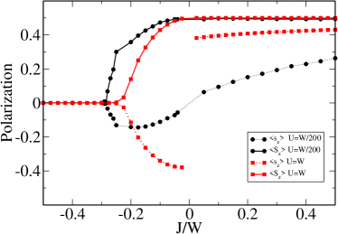
Figure 2: (color online) Antiferromagnetic polarization at half-filling and $T=0$ as function of the coupling $J$ between spins and band electrons. Circles were calculated for $U/W=1/200$, corresponding approximately to $U=0$, squares for $U=W$.

In Fig. 2 are collected results for the polarization $\langle s_{z}\rangle=\frac{1}{2}(n_{\uparrow}-n_{\downarrow})$ of the band electrons and $\langle S_{z}\rangle$ of the local spin. One can see in Fig. 2 two curves corresponding to $U\approx 0$ (circles) and $U=W$ (squares). For large negative $J$ there is no magnetic order. The system forms a Kondo-insulator, locally quenching all moments. Within DMFT we find for the critical value of the coupling at $U=0$ $J_{c}/t\approx-0.3W/t=-1.2$ which is consistent with long-known results.Lacroix and Cyrot (1979) With increasing $U$, this value is shifted to somewhat smaller absolute values $|J|$.

For $J>J_{c}$ antiferromagnetic order can emerge before all moments have been quenched locally. Quite generally, we observe that the polarization $\langle s_{z}\rangle$ of the band states and $\langle S_{z}\rangle$ of the local spins are opposite in sign for $J<0$. Around the critical value $J_{c}$ the resulting total polarization $\langle s_{z}+S_{z}\rangle$ thus is very small, although both contributions can already have rather sizable values. This result is quite interesting, in particular in view of the so-called small-moment antiferromagnetism observed in several rare-earth compounds.

Obviously, for $U=0$ there is no antiferromagnetic order at $J=0$; however, even for very small $|J/W|\ll 1$ the local spins are almost fully polarized, $\langle S_{z}\rangle\approx 0.5$. On the other hand, the polarization of the conduction electrons $\langle s_{z}\rangle$ goes smoothly through zero. We can thus identify this range of $J$ values as corresponding to the RKKY regime, where the local spins are fully polarized and the band electrons show a polarization proportional to the “effective field” $\sim J\langle S_{z}\rangle$ provided by the local spins. In this region we also observe that the magnetic properties of the system are roughly independent of the sign of $J$, as predicted by RKKY.

On the other hand, the behavior in the vicinity of $J_{c}$ cannot be understood in terms of RKKY any more, although $|J_{c}|=0.3W$ is still significantly smaller than $W$ and one might expect the perturbational arguments to be still valid. However, the physical properties are radically different for $J<0$ and $J>0$, as no critical point exists for $J>0$ and the model always is in the fully polarized state.

For $U>0$ there is antiferromagnetic order even at $J=0$, which represents the pure Hubbard model.Georges et al. (1996); pruschke:05 As mentioned before, for $J<0$ spin and electron polarizations are antiparallel while for $J>0$ both orientations are parallel. Due to to numerical errors we were not able to determine the behavior as $J\rightarrow 0$. Even with as many as $4000$ states kept in each NRG step DMFT+NRG calculations did not converge but showed strong fluctuation for $|J/W|<0.04$. The results obtained nevertheless suggest a jump at $J=0$. Again, as $J\to 0^{-}$, the net polarization $\langle s_{z}+S_{z}\rangle$ is strongly reduced from the almost full values for each individual part.

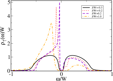
Figure 3: (color online) Spectral function for the majority spin at half filling for $U/W=1/200$ and temperature $T/W=2.3\cdot 10^{-4}$.

Fig. 3 shows the majority spectral functions for $U/W=1/200$ and different $J$. All calculations show a gap at $\omega=0$, characteristic for an insulating behavior. The solid line represents the results for a large antiferromagnetic coupling, i.e. in the Kondo insulating state. The spectral function agrees with the typical result for paramagnetic phase of a Kondo-insulator. The remaining lines correspond to $J>J_{c}$. The dotted and dashed lines correspond to the same value $|J|$, however with opposite signs. The general shape is that of a weak-coupling antiferromagnetZitzler et al. (2006) with the characteristic square-root van-Hove singularities at the gap edges. Note that for $J<0$ we find a shallow shoulder for $\omega>0$ which quite likely is the remnant of a quasiparticle peak due to the Kondo effect expected in this regime.Peters and Pruschke (2056) This is again a sign, that already for moderate values of $J$ the physical properties are significantly different for $J<0$ and $J>0$, i.e. cannot be understood by pure RKKY physics.

The dotted-dashed line in Fig. 3 corresponds to a large ferromagnetic coupling. Here, life-time effects due to a large self-energy already substantially dominate the spectrum.

III.2 Doped model at $U=0$

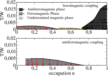
Figure 4: (color online) Magnetic phase diagrams for $U=0$ and $|J|=W/2$ as function of filling and temperature. The upper (lower) panel shows the results for ferromagnetic (antiferromagnetic) coupling. Lines are meant as guide to the eyes. For ferromagnetic coupling a magnetic phase exists between $0.45<n<0.7$, whose nature could not be determined (see text). The number of states kept during NRG calculation was increased at phase boundaries.

Figure 4 shows the magnetic phases of the Kondo-lattice model at $U=0$ as function of filling $n$ and temperature calculated within DMFT for a Kondo coupling $|J|=W/2$. Note that this value is already larger than the critical value $J_{c}$ at half filling, thus we expect that for $J<0$ the physics is governed by local quenching of the moments close to half filling.

The upper panel in Fig. 4 shows the model with ferromagnetic coupling, while the lower one displays the results for antiferromagnetic coupling. In the ferromagnetic Kondo-lattice model we find an antiferromagnetic phase around half-filling $n>0.7$, and a ferromagnetic phase for $n<0.45$. The location of phase boundary of the ferromagnet at $T=0$ appears to agree very well with RKKY prediction from Fig. 1, where the coupling between the localized spins within DMFT becomes ferromagnetic for $n<0.45$. We have focused in our work on homogeneous ferromagnetic-, antiferromagnetic Néel- and paramagnetic states. Between $0.45<n<0.7$ calculations showed also significant magnetic response. But neither a ferromagnetic nor an antiferromagnetic Néelstate could be stabilized. The real nature of this phase could not yet be clarified in our calculations, but one might argue that one should expect some type of incommensurate order. In fact, the magnetic phase diagram of the Kondo-lattice model has been analyzed by a number of other authors.Lacroix and Cyrot (1979); Fazekas and Müller-Hartmann (1991); Yunoki et al. (1998); Dagotto et al. (1998); Nagai et al. (1999); Santos and Nolting (2002); Nolting, Müller, Sanots (2003); Yin (2003); Kienert and Nolting (2006); Fishman et. al. (2006) In addition to the conventional homogeneous ferromagnet and Néel antiferromagnet other magnetic phases like incommensurate, chiral and short range ordered phases were analyzed for $0.5<n<1.0$ in these studies and found to be stable in the regime where our calculations fail to converge.

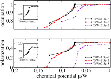
Figure 5: (color online) Occupancy (upper panel) and polarization (lower panel) for the antiferromagnetic solution around half filling as function of chemical potential $\mu$ for different temperatures. Other parameters as in Fig. 4.

For the antiferromagnet close to $n=1$, several authorsYunoki et al. (1998); Dagotto et al. (1998); Nagai et al. (1999); Yin (2003); Kienert and Nolting (2006) also reported phase separation between antiferromagnetism at half-filling and phases away from half-filling. Figure 5 shows our results for the occupancy and polarization in the antiferromagnetic phase as function of the chemical potential $\mu$ for different temperatures. We see that with decreasing temperature the slope of the curves for $n\to 1.0$ get larger and larger. However, even for the lowest temperature we could stabilize every occupation number $n<1.0$, even if there is a large slope for $n\to 1.0$. Increasing the numerical accuracy by for example keeping more states per NRG step also tend to increase the slope further. However, we did never observe a clear jump of the occupation at a critical value of the chemical potential. Note, however, that we cannot rule out phase separation at $T=0$ from our numerical results.

The lower panel in figure 4 shows the phase diagram of the antiferromagnetic Kondo-lattice model. Here our results yield only evidence for a ferromagnetic phase. In contrast to the ferromagnetic Kondo-lattice model, this phase reaches to significantly higher occupations and temperatures; the antiferromagnetic coupling seems to stabilize ferromagnetic order. This behavior as well as the rather large critical value for $n$ at $T=0$ cannot be explained within the RKKY picture. Furthermore, the quite likely incommensurate phase neighboring the ferromagnet for $J>0$ is absent here. For $n\to 0$ we could not stablilize a magnetic phase any more due to numerical problems connected with the small filling.

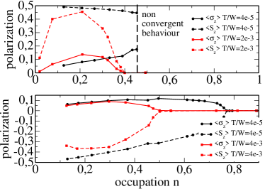
Figure 6: (color online) Polarization of the ferromagnetic solutions. The upper (lower) panel corresponds to ferromagnetic (antiferromagnetic) coupling. Other parameters as in Fig. 4.

The previous observations are further substantiated by the results in Fig. 6, where we show the ferromagnetic polarizations for ferromagnetic (upper panel) and antiferromagnetic (lower panel) coupling parameter. The circles correspond to a very low temperature, squares to a temperature near the transition into the paramagnetic state. Full lines represent $\langle s_{z}\rangle$, dashed lines $\langle S_{z}\rangle$. For $J>0$ and temperatures above the critical temperature for the “incommensurate” phase, both $\langle s_{z}\rangle$ and $\langle S_{z}\rangle$ show a similar behavior as function of doping. In particular, they vanish smoothly as $n\to n_{c}$, indicating a second order phase transition. For very low $T$, on the other hand, $\langle S_{z}\rangle$ remains almost constant at the fully polarized value until we reach the phase boundary to the “incommensurate” phase at $n_{c}\approx 0.45$. At the same time, $\langle s_{z}\rangle$ monotonically increases with filling up to $n_{c}$. Although we cannot determine the true structure of the phase for $n>n_{c}$, its existence seems to be connected to the peculiar behavior of $\langle s_{z}\rangle$ rather than with $\langle S_{z}\rangle$, i.e. is primarily driven by the itinerant electrons. We are currently further investigating this phase transition by including magnetic structures other than the Néel state in our calculations.

For antiferromagnetic coupling (lower panel of Fig. 6) we find a critical $n_{c}$ increasing with temperature, where the ferromagnetic metal becomes a Kondo insulator. Note that for $T/W=4\cdot 10^{-5}$ we are effectively in the ground state. Further lowering the temperature does not change the phase diagram any more. Both $\langle s_{z}\rangle$ and $\langle S_{z}\rangle$ appear to vanish smoothly, too, thus again indicating a second order phase transition.

Choosing $|J|<|J_{c}|$ does not modify the general structure of the phase diagram for ferromagnetic coupling. The results for antiferromagnetic coupling, of course, do change, in particular close to half filling, where now an antiferromagnetic phase appears, too. While the overall structure of the phase diagram is now similar to the case $J>0$ in Fig. 4 upper panel, the values for $n_{c}^{(FM)}$ are still enhanced with respect to the RKKY prediction.

III.3 Finite Coulomb interaction $U=W/2$

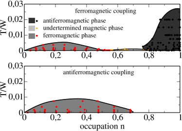
Figure 7: (color online) Magnetic phase diagrams for $U=W/2$ and $|J|=W/2$ as function of filling and temperature. The upper (lower) panel shows results for ferromagnetic (antiferromagnetic) coupling. Lines are meant as guides to the eye. For ferromagnetic coupling a magnetic phase exists between $0.5<n<0.8$, whose nature could not be determined (see text). The number of states kept during NRG calculation was increased at phase boundaries.

Let us now turn to the model with finite on-site Coulomb interaction. We present results for fixed $U=|J|=W/2$, changing these parameters modifies the observations quantitatively but not qualitatively. The phase diagrams for ferromagnetic (upper panel) and antiferomagnetic (lower panel) coupling are shown in Fig. 7. As for $U=0$, we find both an antiferromagnetic phase around half filling and a ferromagnetic phase for larger doping in the ferromagnetic Kondo-lattice model. The critical values have changed to $n_{c}^{(AF)}\approx 0.8$ and $n_{c}^{(FM)}\approx 0.53$ for $T=0$, indicating that local correlations additionally stabilize ferromagnetic order but destabilize antiferromagnetic for $J>0$, in accordance with the anticipated variation of $J_{RKKY}$ with $U$.

For the ferromagnetic Kondo lattice model we again find between the ferromagnetic phase for $n<0.53$ and the antiferromagnetic for $0.8<n<1$ a magnetic phase whose nature could not be determined for the same reasons as for $U=0$. Guided by our observations for $U=0$ and a comparison to other studies by other groups, one can again assume the appearance of an incommensurate magnetic phase like a spin wave or a chiral phase. From quantum Monte-Carlo studies Freericks and Jarrell (1995) for the conventional Hubbard model an incommensurate phase can indeed be anticipated in this parameter regime.

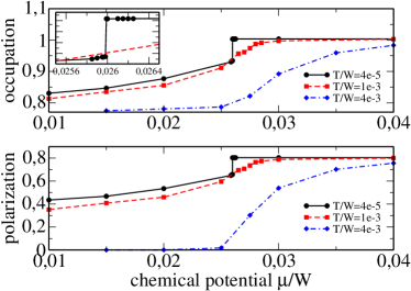
Figure 8: (color online) Occupancy (upper panel) and polarization (lower panel) for the antiferromagnetic solution around half filling as function of chemical potential $\mu$ for different temperatures. chemical potential $\mu$. Other parameters as in Fig. 7.

Figure 8 shows occupation and polarization as function of the chemical potential $\mu$ for different temperatures. For high-temperatures, squares and triangles, there is a smooth crossover from half-filling to lower occupancies, as for $U=0$ (cf. Fig. 5). However, in contrast to the indecisive results at $U=0$, we observe clear evidence for phase separation at $T/W=4\cdot 10^{-5}$, circles, this time. There exists a critical value $\mu_{crit}$, where both occupation and polarization jump from their values at half-filling to a smaller occupancy and polarization. We therefore have phase separation between the antiferromagnetic insulator at half-filling and an antiferromagnetic metal with a lower occupancy. Note that one also finds phase separation in the conventional Hubbard model, which here however occurs between an antiferromagnetic insulator with $n=1$ and a paramagnet with $n<n_{c}^{(AF)}$.Zitzler et al. (2006)

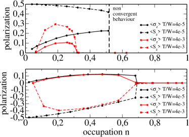
Figure 9: (color online) Polarization of the ferromagnetic solutions. The upper (lower) panel corresponds to ferromagnetic (antiferromagnetic) coupling. Other parameters as in Fig. 7.

The dependence of the polarization on $n$ and $T$ in the ferromagnetic phase for the present values of $U$ and $|J|$ is shown in Fig. 9 for $J>0$ (upper panel) and $J<0$ (lower panel). As in Fig. 6, full lines represent $\langle s_{z}\rangle$ and dashed lines $\langle S_{z}\rangle$. For high temperatures (squares) we again find second order phase transitions, indicated by the smooth simultaneous vanishing of both $\langle s_{z}\rangle$ and $\langle S_{z}\rangle$, while for low $T$ (circles) and $J>0$ the peculiar behavior at the phase boundary to the “incommensurate” phase already seen in Fig. 6 is observed.

A markable difference to the behavior for $U=0$ collected in Fig. 6 can be observed for antiferromagnetic coupling $J<0$. Here, the polarization now vanishes discontinously at $n_{c}^{(FM)}$ for $T\to 0$, indicating a first order phase transition in contrast to the second order type observed for $U=0$. Thus, while the results at $U=0$ would predict a quantum critical point at $n_{c}^{(FM)}$, such a scenario is obvioulsy destroyed by Coulomb correlations in the conduction band, at least within DMFT.

Note that for the bare Hubbard model no ferromagnetic phase exists in this parameter regime for a bipartite lattice. It is thus clearly the spin-electron interaction which leads to ferromagnetism. Our results are consistent with earlier studies by other groups, who however treated the electron-electron interaction in an effective medium approach,Nolting et al. (2003); Kienert et al. (2003); Golosov (2005); Stier and Nolting (2007) while we are able to treat the on-site correlations exactly within DMFT and NRG. Especially our Curie temperatures are located in the same range as in these earlier studies.

A possible reason for the tendency of both finite $U$ and negative $J$ to stabilize ferromagnetism is the strong asymmetry induced by $U$ and $J$Tasaki (1998); Ulmke (1998). As can be seen from Fig. 10, this effect is most pronounced

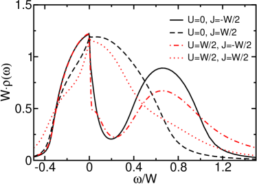
Figure 10: (color online) DOS for $n=0.6$, $T=4\cdot 10^{-5}$, $U=0$, $W/2$ and $J=\pm W/2$.

for $J<0$. For $J>0$, a weaker, but nonetheless significant redistribution of spectral weight is observed, which can explain the increase of $n_{c}^{(FM)}$ here, too.

IV Summary

In this paper we discussed the magnetic properties of the extended Kondo lattice model, where in addition to an exchange coupling between itinerant states and localized spins the band electrons are subject to a local Coulomb interaction. Such a model is expected to describe the properties of e.g. transition metal compounds, where part of the $d$-states are localized in the crystalline environment due Coulomb correlations and form a local spin which couples to the remaining, usually itinerant $d$-states either due to Hund’s exchange or hybridization.

These materials typically have a rich magnetic phase diagram, and it is an interesting question, how these two interactions cooperate or compete in driving different magnetic phases. A particularly interesting question in this respect is, to what extent, qualitatively and quantitatively, the concept of the RKKY approximation of an effective interaction between the local spins mediated by the itinerant conduction states holds.

We treat the model within DMFT, using NRG as solver for the effective impurity problem. The calculations were done for a bipartite lattice, allowing for homogeneous ferromagnetism and Néel antiferromagnetism. At half filling, we find an antiferromagnetic phase, as expected, for all ferromagnetic Kondo couplings $J>0$. For antiferromagnetic coupling $J<0$, there exists a critical $J_{c}$, where the system becomes a paramagnetic Kondo insulator.doniach:77

For $J>J_{c}$, this antiferromagnetic phase prevails for finite doping up to a critical filling $n_{c}^{(AF)}$ depending on $J$ and the local Coulomb interaction $U$. For finite $U$ and $J>0$, we in addition find phase separation between the antiferromagnetic insulator with $n=1$ and an antiferromagnetic metal with $n<1$. For $U=0$ we find no convincing evidence that such a phase separation exists, too, but the numerical results are not sufficiently clear to rule it out either. For $J<J_{c}$ no antiferromagnetic phase exists at all.

Below a second critical filling $n_{c}^{(FM)}$ a homogeneous ferromagnet is found. Quite interestingly, the extent and stability of this phase is increased by both a finite $U$ and an antiferromagnetic $J$. The reason for this stabilization can quite likely be traced back to the introduction of a strong asymmetric redistribution of spectral weight in the electronic spectral function. An interesting aspect in connection with quantum critical points in e.g. ferromagnetic heavy fermion compounds is that for antiferromagnetic Kondo exchange a finite Coulomb correlation among the conduction states has the tendency to change the order of the phase transition at $n_{c}^{(FM)}$ from second order without correlation to first order with correlations.

We find that for ferromagnetic Kondo coupling $J$ the predictions by RKKY can be used to at least qualitatively account for the different phases. For moderate and large $J<0$, however, RKKY cannot even qualitatively predict the phases correctly, underestimating the ferromagnetic phase grossly. Moreover, the variations of the polarizations of the local spin and bandelectrons seem to follow RKKY for very small $|J|$, but already deviate substantially for moderate values.