Quantum Attractor Flows

Abstract:

Motivated by the interpretation of the Ooguri-Strominger-Vafa conjecture as a holographic correspondence in the mini-superspace approximation, we study the radial quantization of stationary, spherically symmetric black holes in four dimensions. A key ingredient is the classical equivalence between the radial evolution equation and geodesic motion of a fiducial particle on the moduli space $\cM^{*}_{3}$ of the three-dimensional theory after reduction along the time direction. In the case of $\cN=2$ supergravity, $\cM^{*}_{3}$ is a para-quaternionic-Kähler manifold; in this case, we show that BPS black holes correspond to a particular class of geodesics which lift holomorphically to the twistor space $\cZ$ of $\cM^{*}_{3}$, and identify $\cZ$ as the BPS phase space. We give a natural quantization of the BPS phase space in terms of the sheaf cohomology of $\cZ$, and compute the exact wave function of a BPS black hole with fixed electric and magnetic charges in this framework. We comment on the relation to the topological string amplitude, extensions to $\cN>2$ supergravity theories, and applications to automorphic black hole partition functions.

1 Introduction

In view of the inherent difficulties in quantizing Einstein’s gravity, mini-superspace models of quantum gravity, where all but a finite number of degrees of freedom consistent with certain symmetries are retained, have been a popular subject of study, particularly in quantum cosmology. A space-like analogue of these cosmological models, the radial quantization of static, spherically symmetric black holes in Einstein and Einstein-Maxwell gravity has also been much studied [1, 2, 3, 4, 5, 6]. In the present work we instill supersymmetry in these early treatments and lay out a quantization scheme for stationary, spherically symmetric solutions of four-dimensional ${\cal N}=2$ supergravity. Our motivation stems from recent developments in black hole and string physics, which we now briefly review.

1.1 Motivation

The microscopic origin of the geometric entropy of supersymmetric black holes in type IIA string theory compactified on a Calabi-Yau three-fold $Y$ can be investigated by virtue of several simplifying properties:

• The “attractor phenomenon” [7, 8, 9] implies that the entropy and scalar fields at the horizon (hence the Kähler moduli of $Y$) are functions of the electric and magnetic charges only.

• Since BPS black holes are extremal, they are not subject to Hawking evaporation, yet their entropy can be made as large as desired by increasing their charges.

• Being supersymmetric, they are expected to correspond to exact zero-energy eigen-states (or eigen-matrices) of the microscopic Hamiltonian.

• Due to the tree-level decoupling between vector multiplets and hypermultiplets, the string coupling may be made as small as desired, such that micro-states can be described as a gas of weakly coupled open strings or membranes, whose microscopic entropy can be reliably computed on combinatorial grounds.

Taken together, these simplifications have led to a clear microscopic derivation of the Bekenstein-Hawking entropy of a class of BPS black holes [10, 11, 12], accurate in the limit of large charges (even reproducing the first subleading correction in the M-theory approach [13]). The modern version of this argument uses holographic duality between M-theory on the attractor near-horizon geometry $[AdS_{3}/\Gamma]\times S^{2}\times Y_{*}$ of a five-dimensional black string whose reduction to four dimensions produces the black hole of interest, and a two-dimensional superconformal field theory at the boundary of $AdS_{3}$ (see e.g. [14, 15] for reviews and references).

Recently, there have been many efforts to extend this agreement beyond the large charge regime. On the macroscopic side the geometric entropy, including the effects of an infinite series of higher-derivative BPS couplings in the low energy effective action, has been computed [16, 17, 18]; the result takes a particularly simple form when expressed in terms of a mixed thermodynamical ensemble with fixed magnetic charges $p^{I}$ and electric potentials $\phi^{I}$ [19]. Combined with the relation between higher-derivative BPS couplings and the topological string amplitude on the Calabi-Yau threefold $Y$, it suggests a intriguing relation [19]

$$\Omega(p^{I},q_{I})\sim\int d\phi^{I}\ \Psi_{\rm top}^{*}(p^{I}-i\phi^{I})\ \Psi_{\rm top}(p^{I}+i\phi^{I})\ e^{\pi\phi^{I}q_{I}}\,,$$ (1.1)

between the indexed degeneracies $\Omega(p^{I},q_{I})$ of BPS states with magnetic and electric charges $(p^{I},q_{I})$, and the topological string amplitude $\Psi_{\rm top}$; the latter should be understood as a wave function in the real (background-independent) polarization ensuring covariance under a change of electric-magnetic duality frame [20, 21, 22, 23]. The equality in (1.1) was conjectured to hold to all orders in an expansion at large charges, as supported by various explicit checks for compact [24, 25] and non-compact $Y$ [26, 27, 28]. The relation (1.1) has been derived recently by evaluating the elliptic genus of M-theory in the above near-horizon geometry [29, 30, 31, 32] (see also [33] for an alternative approach using D6-branes).

Both these recent discussions of the subleading corrections to the entropy, as well as the original derivations in [11, 12, 13], rely on the possibility of lifting the four-dimensional black hole to a five-dimensional black string: while this is indeed possible for vanishing or unit $D6$-brane charge, in general the five-dimensional parent is a black hole in a singular Taub-NUT background, possibly accompanied by a black ring [34, 35]. In fact, standard holography arguments suggest that it should be possible to describe the spectrum of black hole micro-states in terms of superconformal quantum mechanics on the (disconnected) boundary of the near-horizon geometry $AdS_{2}\times S^{2}\times Y_{*}$. Unfortunately, this superconformal quantum mechanics has remained vexingly elusive (see however [36, 37] for some recent progress).

Lacking a concrete definition of the superconformal quantum mechanics on the boundary of $AdS_{2}$, it is worthwhile trying to obtain indirect information on its spectrum using the AdS/CFT correspondence. Specifically, the cylinder-like topology of thermal $AdS_{2}$ suggests, in analogy with the familiar open/closed string duality, that it should be possible to derive the partition function of the black hole micro-states – the “open string channel” – as an overlap of wave functions in a radial quantization scheme – the “closed string channel” – see Figure 1. Performing a radial quantization of gravity is hardly doable in general, but becomes tractable in a “mini-superspace” truncation where only stationary spherically symmetric geometries are retained.

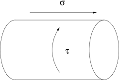
Figure 1: Left: the cylinder amplitude in string theory can be viewed either as a trace over the open string Hilbert space (quantizing along $\tau$) channel) or as an inner product between two wave functions in the closed string Hilbert space (quantizing along $\sigma$). Right: The global geometry of Lorentzian $AdS_{2}$ has the topology of a strip; its Euclidean continuation at finite temperature becomes a cylinder. $\tau$ and $t$ are the global and Poincaré time, respectively.

It has been proposed to interpret (1.1) in just this way [38]: regard the left-hand side as the partition function in the Hilbert space of BPS black holes with given values of the charges (and zero Hamiltonian), and the right-hand side as the overlap of two wave functions in the Hilbert space of spherically symmetric BPS geometries. To spell this out, analytically continue $\phi^{I}=i\chi^{I}$ to the imaginary axis and define

$$\Psi_{p,q}^{\pm}(\chi)\equiv e^{\pm\frac{i\pi\chi q}{2}}\ \Psi_{\rm top}(\chi\mp p)\equiv V_{p,q}^{\pm}\cdot\Psi_{\rm top}(\chi)\ .$$ (1.2)

Equation (1.1) may then be rewritten more suggestively as an overlap of two wave functions,

$$\Omega(p,q)\sim\int d\chi\ [\Psi^{-}_{p,q}(\chi)]^{*}\ \Psi_{p,q}^{+}(\chi)\ .$$ (1.3)

This interpretation assumes one can view the topological amplitude $\Psi_{\rm top}$ as a wave function for the radial quantization of spherically symmetric geometries; if true, it would provide a physical interpretation for the wave function property of the topological string partition function, observed at a formal level in [20].

While the mini-superspace approximation is usually at best ill-controlled, one may hope that, for the purpose of the indexed partition function of BPS black holes, the truncation to BPS ground states in the radial channel may be justified. In this respect, note that the quantization of BPS configurations has been applied in various set-ups [39, 40, 41, 42, 43], and used for a derivation of the entropy of two-charge black holes [44].

Finally, we note that further interest in the quantization of attractor flows arises from the analogy between black hole attractor equations and the equations that determine supersymmetric vacua in flux compactifications, and possible applications of the black hole wave function to vacuum selection in string theory [38].

1.2 Summary and Outline

Some of our results have been announced in [45, 15]: the key observation, explained in Section 2, is the equivalence [46] between the radial equations of motion for stationary, spherically symmetric solutions, and the geodesic motion of a fiducial superparticle on a pseudo-Riemannian manifold ${\cal M}_{3}^{*}$; the latter arises by supplementing the four-dimensional moduli space ${\cal M}_{4}$ with the various scalars arising in the dimensional reduction along the time direction. The electric and magnetic charges $(q_{I},p^{I})$ of the black hole, the ADM mass $m$ as well as the NUT charge $k$ are conserved Noether charges associated to isometries of ${\cal M}_{3}^{*}$, whose Poisson brackets obey an extended Heisenberg algebra (2.7). Extremal black holes correspond to light-like geodesics on ${\cal M}_{3}^{*}$. The phase space of stationary, spherically symmetric solutions is the cotangent bundle $T^{*}({\cal M}_{3}^{*})$, or one of its symplectic quotients when some conserved charges are held fixed. Quantization is then in principle clear: the Hilbert space for radial quantization is the space of square-integrable functions on ${\cal M}_{3}^{*}$, subject to the Hamiltonian and charge constraints. In Subsection 2.3, we briefly outline how physical observables can be extracted from a wave function in this Hilbert space; we note however that conserved charges alone do not select a unique wave function.

This situation is vastly improved when restricting to BPS solutions. As we show in Section 3, supersymmetry strongly restricts the allowed momentum along the geodesic, effectively removing half the degrees of freedom. In the context of ${\cal N}=2$ supergravity, ${\cal M}_{3}^{*}$ is an analytic continuation of a quaternionic-Kähler space ${\cal M}_{3}$ obtained by the $c$-map construction from the four-dimensional special Kähler moduli space ${\cal M}_{4}$. Supersymmetry requires the momentum to satisfy certain quadratic constraints (3.7b) built from the quaternionic vielbein of ${\cal M}_{3}$. The geometric structure of the BPS phase space is however obscure in this formulation.

Instead the supersymmetry constraint is better expressed by introducing the twistor space $\cZ$ – a two-sphere bundle over ${\cal M}_{3}$ which carries a canonical complex structure, as well as a Kähler-Einstein metric. It is also useful to introduce the Swann bundle $\mathcal{S}$ over ${\cal M}_{3}$, which is a line bundle over $\cZ$ with a hyperkähler, $SU(2)$ and scale invariant metric. Physically, the $S^{2}$ or $\mathbb{R}^{4}$ fiber of $\cZ$ or $\mathcal{S}$, respectively, over ${\cal M}_{3}$ keeps track of the Killing spinor preserved by the black hole. Supersymmetric trajectories on the base $\cM_{3}$ then simply correspond to “holomorphic” geodesics in one complex structure on $\mathcal{S}$ (i.e. trajectories whose tangent vector is holomorphic at any point), with no angular momentum in the fiber. These BPS geodesics descend to holomorphic geodesics on $\cZ$. The BPS phase space is then the twistor space $\cZ$ itself equipped with its Kähler form. Thus, it is roughly twice as small as the non-BPS phase space $T^{*}({\cal M}_{3}^{*})$.

With this reformulation at hand quantization is again in principle clear: the BPS Hilbert space should be the Kähler quantization of the twistor space $\cZ$. Technically, this is complicated by the fact that $\cZ$ does not admit non-trivial holomorphic functions, and moreover has indefinite signature, due to the negative curvature of the base $\cM_{3}$. Moreover, it should be possible to view the BPS Hilbert space as a subspace of the unconstrained Hilbert space $L^{2}(G/K)$, determined by generalized harmonicity constraints (3.37) quantizing the classical quadratic constraints (3.7b).

There is a natural conjecture that addresses these concerns all at once: the BPS Hilbert space should be the sheaf cohomology group $H^{1}(\cZ,{\cal O}(-\ell))$ for appropriate $\ell$. Indeed, there exists a generalized Penrose transform which relates classes in $H^{1}(\cZ,$ ${\cal O}(-\ell))$ to functions on the base $\cM_{3}$ solving exactly these partial differential equations [47, 48, 49]. A special case of this is the standard Penrose transform, which relates a cohomology class on a subset of ${\mathbb{C}}{\mathbb{P}}^{3}$ to a solution of the conformal Laplacian on a subset of $S^{4}$ (see [50, 51]). The value of $\ell$ determines the spin of the wave function on $\cM_{3}$, and could in principle be computed by a careful quantization of the fermions in the one-dimensional non-linear sigma model, which we defer to a forthcoming publication [52].

In contrast to the non-BPS case, specifying the conserved charges $p^{I},q_{I}$ (at vanishing NUT charge $k=0$) now determines a unique wave function $\Psi_{p,q}$, a plane wave in the complex coordinates on $\cZ$ adapted to the Heisenberg symmetries. Contour integration of the BPS wave function on $\cZ$ leads to the exact wave function (3.43) of a BPS black hole with charges $(p,q)$ as a function of the four-dimensional vector-multiplet moduli, as well as of the scale $U$ of the time direction. The norm of the wave function is maximal at the classical attractor point(s), but is not exponentially suppressed away from them, contrary perhaps to expectations. In fact, the effective Planck constant grows as $e^{-U}$ toward the horizon at $U\to-\infty$, leading to large quantum fluctuations. The implications of this result deserve to be further investigated.

The outline of this paper is as follows. In Section 2 we review the general equivalence between the radial evolution equations for stationary, spherically black holes in 4 dimensions and geodesic flow on the three-dimensional moduli space, and discuss the general features of the radial quantization for non-supersymmetric black holes. In Section 3 we specialize to $\cN=2$ supergravity, show that twistor techniques allow one to characterize the geodesics associated to BPS black holes, propose a natural quantization scheme of the BPS phase space, based on the Kähler quantization of the twistor space, and compute the exact wave function for a BPS black hole in this framework (some of the material in this Section is a review of the results in [49]). We conclude in Section 4 with a discussion of the relation of our wave function to the topological string amplitude, applications to symmetric $\cN=2$ and $\cN>2$ supergravities, and to automorphic counting functions for black hole micro-states, and other directions. In Appendix A we supply details on the reduction of the supersymmetry conditions from 4 to 3 dimensions. In Appendix B we discuss pure $\cN=2$ supergravity in four dimensions. In Appendix C, we comment on supergravity theories with $\cN=4$ and $\cN=8$.

2 Attractor Flows and Geodesic Motion

We begin by reformulating the equations of motion for stationary solutions in four dimensions in terms of a gravity-coupled non-linear sigma-model on an extended moduli space ${\cal M}_{3}^{*}$ in three Euclidean dimensions. By assuming spherical symmetry the problem is further reduced in Subsection 2.2 to the geodesic motion of a fiducial particle on ${\cal M}_{3}^{*}$. In Subsection 2.3 we quantize this mechanical system. No assumption about supersymmetry is made in this Section.

2.1 Stationary Metrics and Harmonic Maps

We consider Einstein gravity in four dimensions coupled to $n_{A}$ Abelian gauge fields $A_{4}^{I}$ and $n_{S}$ scalar fields $z^{i}$ with action

$$S_{4}=\!\int\!d^{4}x\left[-\frac{1}{2}\sqrt{-\gamma}\ R[\gamma]-g_{ij}\ dz^{i}\!\wedge{}^{\star}\!dz^{j}+F^{I}\!\wedge\!\Big{(}\frac{1}{4}({\rm Im}{\cal N})_{IJ}\wedge{}^{\star}\!F^{J}\!-\frac{1}{8}({\rm Re}{\cal N})_{IJ}F^{J}\Big{)}\right].$$ (2.1)

Here $\gamma$ denotes the four-dimensional metric, $g_{ij}$ ($i=1\dots n_{S}$) the metric on the moduli space ${\cal M}_{4}$ where the (real) scalars $z^{i}$ take their values, $F^{I}=dA_{4}^{I}$ ($I=1\dots n_{A}$) are the field strengths of the Maxwell fields with complexified gauge couplings ${\cal N}_{IJ}(z^{i})=({\cal N}^{IJ})^{-1}$.

Now we restrict our attention to stationary configurations. The most general stationary metric has the form

$$ds_{4}^{2}=-e^{2U}(dt+\omega)^{2}+e^{-2U}ds^{2}_{3}\ ,\quad$$ (2.2)

where the scalar $U$, one-form $\omega$ and line element $ds_{3}^{2}$ are functions on the spatial slice $\Sigma$ and independent of $t$. Similarly we decompose the vector fields as

$$A_{4}^{I}=\zeta^{I}(dt+\omega)+A^{I}_{3}\ ,$$ (2.3)

into pseudo-scalars $\zeta^{I}$ and one-forms $A^{I}_{3}$ defined on $\Sigma$ and assume that the scalars $z^{i}$ are independent of time. The equations of motion for $(U,\omega,ds^{2}_{3},\zeta^{I},A^{I}_{3})$ may be obtained by reducing action $S_{4}$ along the time direction. In three dimensions, the one-forms $A^{I}_{\rm i}$ and $\omega$ can be dualized into axionic scalars $\tilde{\zeta}_{I}$ and $\sigma$. Thus, the four-dimensional theory reduces to a non-linear sigma model coupled to Euclidean gravity,

$$S_{3}=\int\ \ d^{3}x\left(\sqrt{g_{3}}\ R[g_{3}]-g_{mn}\ d\phi^{m}\wedge\star d\phi^{n}\right)\ ,$$ (2.4)

whose the coordinates $\phi^{m}$ on the target space ${\cal M}_{3}^{*}$ include the scalar fields $z^{i}$ from four dimensions together with $U$, $\zeta^{I}$, $\tilde{\zeta}_{I},\sigma$. In contrast to the usual Kaluza-Klein reduction along a space-like direction, the metric $g_{mn}$ on ${\cal M}_{3}^{*}$ has indefinite signature:

$$ds^{2}_{\cM_{3}^{*}} = dU^{2}+\frac{1}{2}g_{ij}dz^{i}dz^{j}+e^{-4U}\left(d\sigma-\tilde{\zeta}_{I}d\zeta^{I}+\zeta^{I}d\tilde{\zeta}_{I}\right)^{2}$$

$$+\frac{1}{2}e^{-2U}\left[({\rm Im}{\cal N})_{IJ}d\zeta^{I}d\zeta^{J}+\,({\rm Im}{\cal N})^{IJ}\left(d\tilde{\zeta}_{I}+({\rm Re}{\cal N})_{IK}d\zeta^{K}\right)\left(d\tilde{\zeta}_{J}+({\rm Re}{\cal N})_{JL}d\zeta^{L}\right)\right]\ ,$$

(recall that $({\rm Im}{\cal N})_{IJ}$ is negative definite). It is related to its Riemannian counterpart ${\cal M}_{3}$ (from standard Kaluza-Klein reduction, see e.g. [53]) by analytic continuation $(\zeta^{I},\tilde{\zeta}_{I})\to i(\zeta^{I},\tilde{\zeta}_{I})$ [45]. Thus, stationary solutions in four dimensions are given by harmonic maps from the (in general curved) three-dimensional spatial slice to ${\cal M}_{3}^{*}$ [46].

Importantly, ${\cal M}_{3}^{*}$ possesses $2n+2$ isometries, reflecting symmetries of the stationary sector of the four-dimensional theory: these are the shift symmetries of $A^{I},\tilde{A}_{I},\omega$, as well as rescalings of time $t$. The Killing vector fields generating these isometries are

$$p^{I}=\partial_{\tilde{\zeta}_{I}}+\zeta^{I}\partial_{\sigma}\ ,\quad q_{I}=\partial_{\zeta^{I}}-\tilde{\zeta}_{I}\partial_{\sigma}\ ,\quad k=\partial_{\sigma}\ ,\quad m=-\partial_{U}-\zeta^{I}\partial_{\zeta^{I}}-\tilde{\zeta}^{I}\partial_{\tilde{\zeta}^{I}}-2\sigma\partial_{\sigma}\ ,$$ (2.6)

and satisfy the Lie algebra

$$[p^{I},q_{J}]=-2\delta^{I}_{J}\ k\ ,\quad[m,p^{I}]=p^{I}\ ,\quad\ [m,q_{I}]=q_{I}\ ,\quad[m,k]=2k\ .$$ (2.7)

This notation anticipates the fact that the associated conserved quantities will be the electric and magnetic charges, NUT charge, and ADM mass of the black hole. In particular, the electric and magnetic charges $p^{I},q_{I}$ satisfy an Heisenberg algebra graded by the ADM mass $m$, with center $k$.

2.2 Stationary, Spherically Symmetric Black Holes and Geodesics

We now further restrict to spherically symmetric solutions. The metric on the spatial slice $\Sigma$ can be parameterized as

$$ds_{3}^{2}=N^{2}(\rho)\ d\rho^{2}+r^{2}(\rho)\ (d\theta^{2}+\sin^{2}\theta\ d\phi^{2})\ ,$$ (2.8)

while the scalars become functions of $\rho$ only. The scalar curvature of $\Sigma$ is

$$\sqrt{g_{3}}\ R^{(3)}=2\sin\theta\left[\frac{(r^{\prime})^{2}}{N}+N-\frac{d}{d\rho}\left(\frac{2rr^{\prime}}{N}\right)\right]\ ,$$ (2.9)

where the prime denotes a $\rho$–derivative. Substituting in (2.4), integrating over the angles $\theta,\phi$ and dropping a total derivative term leads to

$$S_{1}=\int d\rho\ \left[\frac{N}{2}+\frac{1}{2N}\left(r^{\prime 2}-r^{2}\,g_{mn}\,\phi^{\prime m}\,\phi^{\prime n}\right)\right]\ .$$ (2.10)

This Lagrangian describes the motion of a fiducial particle on a cone ${\cal C}$ over the $d=3$ moduli space ${\cal M}_{3}^{*}$. The einbein $N$ on the particle worldline ensures invariance under reparametrizations; its equation of motion enforces the mass shell condition

$$r^{\prime 2}-r^{2}\,g_{mn}\,\phi^{\prime m}\,\phi^{\prime n}=N^{2}\ ,$$ (2.11)

or equivalently, the Wheeler-De Witt (or Hamiltonian) constraint

$$H_{WDW}=(p_{r})^{2}-\frac{1}{r^{2}}g^{mn}p_{m}p_{n}-1\equiv 0\ ,$$ (2.12)

where $p_{r},p_{m}$ are the canonical momenta conjugate to $r$ and $\phi^{m}$.

Solutions are thus massive geodesics on the cone $\mathcal{C}$, with fixed unit mass. The motion separates into geodesic motion on the base of the cone ${\cal M}_{3}^{*}$, with affine parameter $\tau$ such that $d\tau=N\,d\rho/r^{2}$, and motion along the radial direction $r$,

$$(p_{r})^{2}-\frac{C^{2}}{r^{2}}-1\equiv 0\ ,\quad g^{ab}p_{a}p_{b}\equiv C^{2}\ ,$$ (2.13)

where $p_{r}=r^{\prime}/N$ and $p_{m}=r^{2}\phi^{{}^{\prime}m}/N$. It is interesting to note that the radial motion is governed by the same Hamiltonian as in [57, 55], and therefore exhibits one-dimensional conformal invariance

The motion along $r$ is easily integrated in the gauge $N=1$ to

$$r=\frac{C}{\sinh(C\tau)}\ ,\quad\rho=\frac{C}{\tanh(C\tau)}\ .$$ (2.14)

By looking at the behavior of the metric near $\tau=\infty$, it is easy to see that the integration constant $C$ is related to the Hawking temperature $T_{H}$ and black hole entropy $S_{BH}$ through [9]

$$C=2S_{BH}T_{H}\ .$$ (2.15)

Non-extremal black holes have $C>0$ (the opposite sign results in a naked singularity), while extremal black holes correspond to light-like geodesics, with $C=0$. In this case, the first and last term in (2.12) must cancel,

$$r^{\prime}=N\ ,$$ (2.16)

leading to flat spatial slices $\Sigma$. In the gauge $N=1$, Equations (2.14) imply that the affine parameter is the inverse of the radial distance, $\tau=1/r=1/\rho$. While one may dispose of the radial variable $r$ altogether, it is however advantageous to retain it for the purpose of defining observables such as the horizon area, $A_{H}=4\pi e^{-2U}r^{2}|_{U\to-\infty}$ and the ADM mass $m=r(e^{2U}-1)|_{U\to 0}$.

As anticipated in (2.7), the isometries of ${\cal M}_{3}^{*}$ lead to conserved Noether charges,

$$q_{I}\ d\tau = e^{-2U}\left[({\rm Im}{\cal N})_{IJ}d\zeta^{J}+({\rm Re}{\cal N})_{IJ}({\rm Im}{\cal N})^{JL}\left(d\tilde{\zeta}_{L}+({\rm Re}{\cal N})_{LM}d\zeta^{M}\right)\right]-2k\,\tilde{\zeta}_{I}\,,$$

$$p^{I}\ d\tau = e^{-2U}({\rm Im}{\cal N})^{IL}\left(d\tilde{\zeta}_{L}+({\rm Re}{\cal N})_{LM}d\zeta^{M}\right)+2k\,\zeta^{I}\,,$$ (2.17)

$$k\ d\tau\ = 2\,e^{-4U}\left(d\sigma-\zeta^{I}d\tilde{\zeta}_{I}+\tilde{\zeta}^{I}d\zeta_{I}\right)\,,$$

identified as the electric, magnetic and NUT charges $p^{I},q_{I},k$. Their Poisson brackets of course obey the same algebra as the Killing vectors (2.7).

The NUT charge $k$ is related to the off-diagonal term in the metric (2.2) via $\omega=k\cos\theta\ d\phi$. When $k\neq 0$, the metric

$$ds_{4}^{2}=-e^{2U}(dt+k\,\cos\theta\,d\phi)^{2}+e^{-2U}[d\rho^{2}+r^{2}(d\theta^{2}+\sin^{2}\theta\,d\phi^{2})]\,,$$ (2.18)

has closed timelike curves along the compact $\phi$ coordinates near $\theta=0$, all the way from infinity to the horizon. Bona fide black holes have $k=0$, which corresponds to a “classical” limit of the Heisenberg algebra (2.7).

Using the conserved charges (2.2), one may express the Hamiltonian for affinely parameterized geodesic motion on ${\cal M}_{3}^{*}$ as

$$H\equiv p_{m}g^{mn}p_{n}=\frac{1}{4}p_{U}^{2}+\frac{1}{2}p_{z^{i}}g^{ij}p_{z^{j}}-e^{2U}V_{BH}+\frac{1}{4}k^{2}e^{4U}\ ,$$ (2.19)

where $p_{U},p_{z^{i}}$ are the momenta canonically conjugate to $U,z^{i}$,

$$V_{BH}(p,q,z)=-\frac{1}{2}(\hat{q}_{I}-({\rm Re}{\cal N})_{IJ}\hat{p}^{J})({\rm Im}{\cal N})^{IK}(\hat{q}_{K}-({\rm Re}{\cal N})_{KL}\hat{p}^{L})-\frac{1}{2}\hat{p}^{I}({\rm Im}{\cal N})_{IJ}\hat{p}^{J}\,,$$ (2.20)

and

$$\hat{p}^{I}=p^{I}-2k\zeta^{I}\ ,\quad\hat{q}_{I}=q_{I}+2k\tilde{\zeta}_{I}\ .\quad$$ (2.21)

Following [9], we refer to $V_{BH}$ as the “black hole potential”, keeping in mind that it contributes negatively to the actual potential governing the Hamiltonian motion $V=-e^{2U}V_{BH}+k^{2}e^{4U}$. For $k=0$, the motion along $(\zeta^{I},\tilde{\zeta}_{I},\sigma)$ separates from that along $(U,z^{i})$, effectively producing a potential for these variables. The attractor flow equations, to be discussed in Section 3.1 below, correspond to the restricted class of supersymmetric solutions to (2.19).

2.3 Radial Quantization of Spherically Symmetric Black Holes

Having shown the equivalence between the radial evolution equations for stationary, spherically symmetric geometries and the geodesic motion of a fiducial particle on the cone ${\cal C}$ over ${\cal M}_{3}^{*}$, quantization is now in principle straightforward: replace functions on the classical phase space $T^{*}({\cal C})$ by square integrable wave functions on ${\cal C}$, satisfying mass-shell (Wheeler-De Witt) condition

$$\left[-\frac{\partial^{2}}{\partial r^{2}}+\frac{\Delta_{3}}{r^{2}}-1\right]\Psi(r,U,z^{i};\zeta^{I},\tilde{\zeta}_{I},\sigma)=0\ .$$ (2.22)

Here, $\Delta_{3}$ is the Laplace-Beltrami operator on ${\cal M}_{3}^{*}$, (the quantum analogue of the Hamiltonian $-4H$)

$$\Delta_{3} = \partial_{U}^{2}+\Delta_{4}+e^{4U}\partial_{\sigma}^{2}+2e^{2U}\left[({\rm Im}{\cal N})_{IJ}\,\nabla^{I}\,\nabla^{J}\right.$$

$$\left.+({\rm Im}{\cal N})^{IJ}\left(\nabla_{I}-({\rm Re}{\cal N})_{IK}\nabla^{K}\right)\left(\nabla_{J}-({\rm Re}{\cal N})_{JL}\nabla^{L}\right)\right]\,,$$

while $\Delta_{4}$ is the Laplace-Beltrami operator on the four-dimensional moduli space $\cM_{4}$,

$$\nabla_{I}=\partial_{\zeta^{I}}-\tilde{\zeta}^{I}\partial_{\sigma},\quad\nabla^{I}=\partial_{\tilde{\zeta}_{I}}+\zeta^{I}\partial_{\sigma}\,,$$ (2.24)

and we have rescaled the wave function $\Psi$ with appropriate powers of $r$ and $e^{U}$ to cancel the $\partial_{r}$ and $\partial_{U}$ linear derivatives in the above equations.

The wave equation separates into a Bessel-type equation for the radial direction $r$ and a Laplace equation along ${\cal M}_{3}^{*}$:

$$\Psi(r,U,z^{i};\zeta^{I},\tilde{\zeta}_{I},\sigma)=\sqrt{r}\left[\alpha\ J_{\frac{1}{2}\sqrt{1-4C^{2}}}(r)+\beta\ Y_{\frac{1}{2}\sqrt{1-4C^{2}}}(r)\right]\ \Psi_{C}(U,z^{i},\zeta^{I},\tilde{\zeta}_{I},\sigma)\,,$$ (2.25)

where

$$\left[\Delta_{3}+C^{2}\right]\ \Psi_{C}(U,z^{i},\zeta^{I},\tilde{\zeta}_{I},\sigma)=0\,.$$ (2.26)

In practice, we may also be interested in wave functions which are eigenmodes of the electric and magnetic charge operators, given by the differential operators in (2.6),

$$\Psi_{C}(U,z^{i},\zeta^{I},\tilde{\zeta}_{I},\sigma)=\Psi_{C,p,q}(U,z^{i})\ e^{i(p^{I}\tilde{\zeta}_{I}+q_{I}\zeta^{I})}\,,$$ (2.27)

which is then automatically a zero eigenmode of the NUT charge $k$. Note however that, due to the Heisenberg algebra (2.7), it is impossible to simultaneously diagonalize the ADM mass operator $M$, unless either $p^{I}$ or $q_{I}$ vanish. Equation (2.26) then implies that the wave function $\Psi_{C,p,q}(U,z^{i})$ should satisfy the quantum version of (2.19),

$$\left[\partial_{U}^{2}+\Delta_{4}+4e^{2U}V_{BH}(p,q,z)+C^{2}\right]\ \Psi_{C,p,q}(U,z^{i})=0\,.$$ (2.28)

The wave function $\Psi_{C,p,q}(U,z^{i})$ is the main object of interest in this paper, and describes the quantum fluctuations of the scalars $z^{i}$ as a function of the scale $e^{U}$ of the time direction (i.e. effectively as a function of the distance to the horizon). Alternatively, one may study the full wave function $\Psi_{p,q}(r,U,z^{i})$ as a function of the radius $r$: changing variable from $r$ to $A_{H}=4\pi r^{2}e^{-2U}$ gives access to the quantum fluctuations of the horizon area $A_{H}$. In the absence of supersymmetry, it is hardly surprising that the wave function is not uniquely specified by the charges and extremality parameter, as the condition (2.28) leaves an infinite dimensional Hilbert space.

An important aspect of quantization is the definition of an inner product: as in similar instances of mini-superspace quantization, the $L^{2}$ norm on the space of functions on ${\cal C}$ is inadequate for defining expectation values, since it involves an integration along the “time” direction $r$ at which one is supposed to perform measurements. The customary solution to this problem is to note that (2.22) is a Klein-Gordon-type equation, and to replace the $L^{2}$ norm on ${\cal C}$ by the $r$-independent Wronskian

$$\langle\Psi|\Psi\rangle=\int dU\ dz^{i}\ d\zeta^{I}\ d\tilde{\zeta}_{I}\ d\sigma\,e^{-2(n_{V}+2)U}\sqrt{\det(g_{ij})}\,\Psi^{*}\stackrel{{\scriptstyle\leftrightarrow}}{{\partial_{r}}}\Psi\ .$$ (2.29)

For factorized wave functions (2.25), the resulting norm is proportional to the $L^{2}$ norm on ${\cal M}_{3}^{*}$. A severe malady of this construction is that the above scalar product is not positive definite. The standard remedy is to perform a “second quantization” and replace the wave function $\Psi$ by an operator; a similar procedure can be followed here, in analogy with “third quantization” in quantum cosmology [59]. It is reasonable to expect that this procedure describes multi-centered geometries. Fortunately, as we shall see in the next Section, the situation is much improved for BPS states, since the Klein-Gordon product (2.29) is (formally) positive definite when restricted to this sector.

3 BPS Black Holes in $\cN=2$ Supergravity and Twistors

We now specialize to supersymmetric black holes in ${\cal N}=2$ supergravity. In Subsection 3.1, we review the quaternionic-Kähler geometry of the resulting ${\cal M}_{3}^{*}$, identify the geodesics which correspond to black holes preserving half of the supersymmetries, and recover the known form of the attractor equations. In Subsection 3.2, we outline the construction of the twistor space $\cZ$ and Swann space $\mathcal{S}$ over ${\cal M}_{3}$. These provide the most convenient framework to formulate and solve the BPS conditions. In Subsection 3.3, we show that the phase space of BPS black holes is isomorphic to the twistor space $\cZ$, and that BPS black holes correspond to holomorphic geodesics on $\mathcal{S}$. Finally, in Subsection 3.4 we propose a quantization scheme for spherically symmetric BPS configurations, based on the Penrose transform between cohomology classes valued in a certain holomorphic line bundle on $\cZ$ and solutions of certain second order partial differential equations on the quaternionic-Kähler base ${\cal M}_{3}$. In this framework, we obtain the exact wave function for a BPS black hole with fixed electric and magnetic charges, and discuss some of its properties. While most of the mathematical results in this Section were obtained in [49], our aim here is to illuminate the physics motivations behind these mathematical constructions.

3.1 Attractor Flow and Geodesic Flow

Four-dimensional ${\cal N}=2$ supergravity with $n_{V}$ vector multiplets consists of $n_{S}/2=n_{V}$ complex scalars, $n_{A}=n_{V}+1$ Maxwell fields (including the graviphoton), two gravitini and $n_{V}$ gaugini (hypermultiplets may be safely ignored as they are not sourced by black holes). The couplings in the four-dimensional action (2.1) are determined in terms of a holomorphic prepotential function $F(X^{I})$. The manifold ${\cal M}_{4}$ is a projective special Kähler manifold with Kähler potential

$${\cal K}(z^{i},\bar{z}^{\overline{j}})=-\log K(X,\bar{X})=-\log\left[i\left(\bar{X}^{I}F_{I}-X^{I}\bar{F}_{I}\right)\right]\ ,$$ (3.1)

where $F_{I}:=\partial F(X)/\partial X^{I}$, $I=0\dots n_{V}$, while the gauge kinetic terms are related to the second derivative $\tau_{IJ}:=\partial_{I}\partial_{J}F(X)$ via

$${\cal N}_{IJ}=\bar{\tau}_{IJ}+2i\frac{({\rm Im}\tau\cdot X)_{I}~{}({\rm Im}\tau\cdot X)_{J}}{X\cdot{\rm Im}\tau\cdot X}\ .$$ (3.2)

The scalar manifold ${\cal M}_{3}$ obtained by Kaluza-Klein reduction to three dimensions is a quaternionic-Kähler space, obtained by the “c-map” from the special Kähler manifold ${\cal M}_{4}$ [60, 61, 62, 53]. The analytically continued ${\cal M}_{3}^{*}$ is a para-quaternionic-Kähler space, which we shall refer to as the c^∗-map of ${\cal M}_{4}$. While ${\cal M}_{3}$ has a Riemannian metric with special holonomy $USp(2)\times USp(2n_{V}+2)$, ${\cal M}_{3}^{*}$ has a split signature metric with special holonomy $Sp(2,{\mathbb{R}})\times Sp(2n_{V}+2,{\mathbb{R}})$. As mentioned in the introduction, we work for convenience with the more familiar Riemannian space ${\cal M}_{3}$, leaving the analytic continuation implicit most of the time.

In addition to the bosonic fields appearing in (2.10), the three-dimensional Lagrangian contains also the fermionic partners of $\phi^{m}$ and of the graviton, resulting in $\cN=4$ Euclidean supergravity in three dimensions. Upon further restriction to spherically symmetric solutions, one expects to find fermionic partners for the one-dimensional graviton $N$ and the bosonic fields $r,\phi^{m}$ in $\mathbb{R}^{+}\times{\cal M}_{3}^{*}$, such that the resulting Lagrangian has $\cN=4$ supersymmetry in one dimension. The resulting one-dimensional supergravity model will be presented in [52]. For the present purposes, we only require the supersymmetry transformations of the fermions, the reduction of which is given in Appendix A. To describe this explicitly, let us recall some basic features of quaternionic-Kähler manifolds. The restricted holonomy implies that the complexified tangent bundle of ${\cal M}_{3}$ splits locally as

$$T_{\mathbb{C}}{\cal M}_{3}=E\otimes H\ ,$$ (3.3)

where $E$ and $H$ are complex vector bundles of respective dimensions $2n_{V}+2$ and $2$. This decomposition is preserved by the Levi-Civita connection. The latter decomposes into its $USp(2)$ and $USp(2n_{V}+2)$ parts $p$ and $q$,

$$\Omega_{AA^{\prime}}^{BB^{\prime}}=p_{A^{\prime}}^{B^{\prime}}\delta_{A}^{B}+q^{A}_{B}\delta_{A^{\prime}}^{B^{\prime}}\ ,$$ (3.4)

where $\epsilon_{A^{\prime}B^{\prime}}$, $\epsilon_{AB}$ are the antisymmetric tensors invariant under $USp(2)$, $USp(2n_{V}+2)$ respectively. The change of basis from $T_{\mathbb{C}}{\cal M}_{3}$ to $E\otimes H$ is achieved by a covariantly constant “quaternionic vielbein” $V^{AA^{\prime}}=V^{AA^{\prime}}_{m}d\phi^{m}$ ($A=1,..,2n_{V}+2,\,A^{\prime}=1,2,\,m=1,\dots,4n_{V}+4$), from which one can construct the metric $ds^{2}$, as well as three almost complex structures and their two-forms $\omega^{i}$,

$$ds^{2}=\epsilon_{A^{\prime}B^{\prime}}\ \epsilon_{AB}\ V^{AA^{\prime}}\otimes V^{BB^{\prime}}\ ,\quad\omega^{i}=\epsilon_{A^{\prime}B^{\prime}}\ (\sigma^{i})^{B^{\prime}}_{C^{\prime}}\ \epsilon_{AB}\ V^{AA^{\prime}}\wedge V^{BC^{\prime}}\ .$$ (3.5)

The fermions in the non-linear $\cN=4$ sigma model on $\cM_{3}$ transform under $USp(2n_{V}+2)$ and are $USp(2)$-inert, with supersymmetric variations [52]

$$\delta\chi^{A}=-\frac{1}{N}V_{m}^{AA^{\prime}}\,\stackrel{{\scriptstyle\circ}}{{\phi}}\!{}^{m}\ \epsilon_{A^{\prime}}\ ,$$ (3.6)

where $\stackrel{{\scriptstyle\circ}}{{\phi}}{}^{m}$ is the supercovariant time derivative of $\phi^{m}$, which reduces to the usual time derivative $\phi^{{}^{\prime}m}$ for zero value of the worldline gravitino.

From (3.6), it is apparent that supersymmetric solutions are obtained when $V^{AA^{\prime}}$ has a null eigenvector,

SUSY $$\Leftrightarrow \quad\exists\,\epsilon_{A^{\prime}}\ |\ V^{AA^{\prime}}\epsilon_{A^{\prime}}=0$$ (3.7a)

$$\Leftrightarrow \quad\epsilon_{A^{\prime}B^{\prime}}\,V^{AA^{\prime}}V^{BB^{\prime}}=0\ .$$ (3.7b)

For fixed $\epsilon^{A^{\prime}}$, these are $2n_{V}+2$ conditions on the velocity vector $\phi^{{}^{\prime}m}$ at any point along the geodesic, removing half of the degrees of freedom from the generic trajectories. We now demonstrate that these conditions imply the usual attractor flow equations generalized to include the NUT charge.

For the case of the $c$-map ${\cal M}_{3}$, the quaternionic vielbein was computed explicitly in [53]. After analytic continuation, one obtains

$$V^{AA^{\prime}}=\begin{pmatrix}iu&v\\ e^{a}&iE^{a}\\ -i\bar{E}^{\bar{a}}&\bar{e}^{\bar{a}}\\ -\bar{v}&i\bar{u}\end{pmatrix}\ .$$ (3.8)

where $e^{a}=e^{a}_{i}dz^{i}$ is a vielbein of the special Kähler manifold, $e^{a}_{i}\bar{e}_{\bar{a}\overline{\jmath}}\delta_{a\bar{a}}=g_{i\overline{\jmath}}$, and

$$u = e^{K/2-U}X^{I}\left(d\tilde{\zeta}_{I}+{\cal N}_{IJ}d\zeta^{J}\right)\ ,$$ (3.9a)

$$v = dU-i\,e^{-2U}\left(d\sigma-\tilde{\zeta}^{I}d\zeta_{I}+\zeta^{I}d\tilde{\zeta}_{I}\right)\ ,$$ (3.9b)

$$E^{a} = e^{-U}e^{a}_{i}g^{i\overline{\jmath}}\bar{f}_{\overline{\jmath}}^{I}\left(d\tilde{\zeta}_{I}+{\cal N}_{IJ}d\zeta^{J}\right)\ .$$ (3.9c)

Expressing $d\zeta^{I},d\tilde{\zeta}_{I},d\sigma$ in terms of the conserved charges (2.17), the entries in the quaternionic vielbein may be rewritten as

$$u = ie^{K/2+U}X^{I}\left[q_{I}-2k\tilde{\zeta}_{I}-{\cal N}_{IJ}(p^{J}+2k\zeta^{J})\right]d\tau\ ,\quad$$ (3.10a)

$$v = dU-{i\over 2}e^{2U}k\ d\tau\ ,$$ (3.10b)

$$e^{a} = e^{a}_{i}\ dz^{i}\ ,\quad$$ (3.10c)

$$E^{a} = i\,e^{U}e^{ai}g^{i\overline{\jmath}}\bar{f}_{\overline{\jmath}}^{I}\left[q_{I}-2k\tilde{\zeta}_{I}-{\cal N}_{IJ}(p^{J}+2k\zeta^{J})\right]d\tau\,.$$ (3.10d)

Now we return to the supersymmetry variation of the fermions (3.6): the existence of $\epsilon^{A^{\prime}}$ such that $\delta\chi^{A}$ vanishes implies that the first column of $V$ has to be proportional to the second, hence

$$\frac{dU}{d\tau}-{i\over 2}e^{2U}k = -i\ e^{i\theta}\ e^{K/2+U}\ X^{I}\left(q_{I}-2k\tilde{\zeta}_{I}-{\cal N}_{IJ}(p^{J}+2k\zeta^{J})\right)\,,$$ (3.11a)

$$\frac{dz^{i}}{d\tau} = -i\ e^{i\theta}\ e^{U}\ g^{i\overline{\jmath}}\bar{f}_{\overline{\jmath}}^{I}\left(q_{I}-2k\tilde{\zeta}_{I}-{\cal N}_{IJ}(p^{J}+2k\zeta^{J})\right)\,,$$ (3.11b)

where the phase $\theta$ is determined by requiring the reality of $U$. For vanishing NUT charge, this becomes the well-known attractor flow equations  [7, 8, 9, 64, 65]

$$\frac{dU}{d\tau} = -e^{U}\ |Z|\ ,$$ (3.12a)

$$\frac{dz^{i}}{d\tau} = -2~{}e^{U}~{}g^{i\overline{\jmath}}\partial_{\overline{\jmath}}|Z|\ ,$$ (3.12b)

where $Z$ is the central charge

$$Z(p,q;z^{i},\bar{z}^{\bar{i}})=e^{\mathcal{K}/2}\left(p^{I}F_{I}-q_{I}X^{I}\right)\ .$$ (3.13)

The equivalence between the attractor flow equations on ${\cal M}_{4}$ and supersymmetric geodesic motion on ${\cal M}_{3}$ was observed long ago in [66], and is a consequence of the T-duality between black holes and instantons [67, 68, 69].

Having reproduced the usual form of the attractor equations, we return to the supersymmetry conditions (3.7), and comment on their structure. The quaternionic viel-bein $V^{AA^{\prime}}/d\tau=V^{AA^{\prime}}d\phi^{m}/d\tau$ can be viewed as a $2\times(2n_{V}+2)$ matrix of functions on the unconstrained phase space $T^{*}({\cal M}_{3})$, after expressing the velocity $d\phi^{m}/d\tau$ in terms of the momentum $p_{m}$. Similarly, the quadratic constraints

$$H_{AB}\equiv\epsilon_{A^{\prime}B^{\prime}}\,V^{BB^{\prime}}\,V^{AA^{\prime}}/d\tau^{2}=0\,,$$ (3.14)

are functions on the unconstrained phase space, corresponding to the $2\times 2$ minor determinants of the matrix $V^{AA^{\prime}}$. The constraints $H_{AB}\equiv 0$ are first class, in the sense that their Poisson brackets vanish on the constrained locus. Indeed, computations show that

$$[H_{AB},H_{CD}]=-8\,V_{[AA^{\prime}}\,q^{A^{\prime}}_{B]}{}^{E}_{[C}\,H_{D]E}\,.$$ (3.15)

where $q^{A^{\prime}E}_{BC}$ is the $USp(2n_{V}+2)$ connection, whose one-form index has been traded to $A^{\prime}E$ using the inverse of the quaternionic vielbein. The constraints $H_{AB}$ are not independent however, since the rank one condition on $V^{AA^{\prime}}$ enforces only $2n_{V}+1$ conditions on its $4n_{V}+4$ entries. Since each first class constraint reduces the dimension by two, the real dimension of the BPS phase space is $8n_{V}+8-2(2n_{V}+1)=4n_{V}+6$. The symplectic structure on this space is however obscure from this construction. In the next Section, we show that once the Killing spinor $\epsilon^{A^{\prime}}$ is included, the BPS phase space is realized as the twistor space $\cZ$ of $\cM_{3}$, with complex dimension $2n_{V}+3$.

3.2 Twistor Space and Swann Bundle

The one-dimensional ${\cal N}=4$ non-linear sigma model on $\cM_{3}$ is unusual because the three complex structures responsible for extended supersymmetry are not integrable. This is hardly surprising because the model must also be coupled to worldline gravity. Exactly such a study is underway [52], however, for BPS configurations, this problem can also be circumvented by a standard mathematical construction which physically incorporates the Killing spinor in the black hole geometry, as we discuss further in Subsection 3.3.

Let $\mathcal{S}$ be the total space of the bundle $H$ over ${\cal M}_{3}$. This $4n_{V}+8$ dimensional space, known as the Swann bundle or hyperkähler cone, admits a dilation and $SU(2)$-invariant hyperkähler metric [70, 71]

$$ds^{2}_{\mathcal{S}}=|D\pi|^{2}+\frac{\nu}{4}\,R^{2}\,ds^{2}_{{\cal M}_{3}}\,.$$ (3.16)

Here, $\pi^{A^{\prime}}$ are coordinates in the $\mathbb{R}^{4}$ fiber of $H$, $R^{2}=|\pi^{1}|^{2}+|\pi^{2}|^{2}$ is the $USp(2)$ invariant norm, and $D\pi^{A^{\prime}}$ is the covariant exterior derivative of $\pi^{A^{\prime}}$,

$$D\pi^{A^{\prime}}=d\pi^{A^{\prime}}+p^{A^{\prime}}_{B^{\prime}}\pi^{B^{\prime}}\ ,$$ (3.17)

and $\nu$ is related to the scalar curvature of the base by $R=4n(n+2)\nu$. In particular, $\nu<0$, and $\mathcal{S}$ has quaternionic Lorentzian signature $(1,n_{V}+1)$ and holonomy $USp(2,2n_{V}+2)$. The spin connection $\Omega^{\aleph}_{\beth}$ and the covariantly constant quaternionic vielbein ${\cal V}^{\aleph}$ (where $\aleph\in\{A,A^{\prime}\}$ runs over two more indices than $A$) can be simply obtained from the quaternionic vielbein $V^{AA^{\prime}}$ on the base $\cM_{3}$ via

$${\cal V}^{\aleph}=\begin{pmatrix}D\pi^{A^{\prime}}\\ \hline\cr V^{AA^{\prime}}\pi_{A^{\prime}}\end{pmatrix}\ ,\quad\Omega^{\aleph}_{\beth}=\left(\begin{array}[]{c|c}p^{A^{\prime}}_{B^{\prime}}&V^{AA^{\prime}}\\ \hline\cr V_{BB^{\prime}}&q^{A}_{B}\end{array}\right)\ .$$ (3.18)

The vielbein ${\cal V}^{\aleph}$ gives a set of $(1,0)$-forms on $\mathcal{S}$ (for a particular complex structure), which together with $\bar{\cal V}$ span the cotangent space of $\mathcal{S}$.

It is useful to view the unit sphere $S^{3}$ in $H$ as a Hopf fibration and choose coordinates

$$e^{i\varphi}=\sqrt{\pi^{2}/\bar{\pi}^{2}}\ ,\quad z=\pi^{1}/\pi^{2}\,,$$ (3.19)

on the $U(1)$ fiber and $S^{2}$, respectively. The hyperkähler cone metric (3.16) can then be rewritten as

$$ds^{2}_{\mathcal{S}}=dR^{2}+R^{2}\left(\sigma_{1}^{2}+\sigma_{2}^{2}+\sigma_{3}^{2}+\frac{\nu}{4}ds^{2}_{\cM_{3}}\right)\ ,$$ (3.20)

where the triplet of 1-forms

$$\sigma_{1}+i\sigma_{2}=\frac{dz+{\cal P}}{1+z\bar{z}}\ ,\quad\sigma_{3}=d\varphi-\frac{i}{2(1+z\bar{z})}(\bar{z}dz-zd\bar{z})-\frac{i}{r^{2}}\pi^{A^{\prime}}p_{A^{\prime}}^{B^{\prime}}\bar{\pi}_{B^{\prime}}\,,$$ (3.21)

and $\cal P$ is the projectivized USp(2) connection,

$${\cal P}=p_{2}^{1}+z(p^{1}_{1}-p^{2}_{2})-z^{2}p_{1}^{2}\ .$$ (3.22)

Hence $\mathcal{S}$ is a real cone over a $4n_{V}+7$-dimensional 3-Sasaki space $\mathcal{J}$, which in turn is a $U(1)$ bundle over a $4n_{V}+6$-dimensional “twistor” space $\cZ$ with metric

$$ds^{2}_{\cZ}=\sigma_{1}^{2}+\sigma_{2}^{2}+\frac{\nu}{4}ds^{2}_{\cM_{3}}=\frac{|dz+{\cal P}|^{2}}{(1+\bar{z}z)^{2}}+\frac{\nu}{4}ds^{2}_{\cM_{3}}\,.$$ (3.23)

The twistor space $\cZ$ is an $S^{2}$ bundle over ${\cal M}_{3}$, with complex Lorentzian signature $(1,2n_{V}+2)$, see Figure 2. The twistor space can also be obtained from $\mathcal{S}$ directly as the Kähler quotient by the $U(1)$ symmetry shifting the coordinate $\varphi$ (at unit value of the moment map $|\pi|^{2}$). In particular, it carries a canonical complex structure whose Kähler form is

$$\omega_{\cZ}=i\frac{|dz+{\cal P}|^{2}}{(1+\bar{z}z)^{2}}-\frac{i\nu}{2(1+z\bar{z})}\left[(z+\bar{z})\omega^{1}+i(z-\bar{z})\omega^{2}+(1-z\bar{z})\omega^{3}\right]\ ,$$ (3.24)

where $\omega_{i}$ are the quaternionic 2-forms in (3.5).

Figure 2: Bundles over the quaternionic-Kähler space $\cM_{3}$.

Isometries on $\cM_{3}$ lift to holomorphic isometries on $\cZ$ [72, 73], and tri-holomorphic isometries on $\mathcal{S}$. A set of complex coordinates $\xi^{I},{\tilde{\xi}}_{I},\alpha$ on the Swann bundle $\mathcal{S}$ and twistor space $\cZ$ adapted to the Heisenberg symmetries was constructed in [49]. In terms of these coordinates, the complexified Heisenberg algebra acts as

$$P^{I}=\partial_{{\tilde{\xi}}_{I}}-\xi^{I}\partial_{\alpha}\ ,\quad Q_{I}=-\partial_{\xi^{I}}-{\tilde{\xi}}_{I}\partial_{\alpha}\ ,\quad K=\partial_{\alpha}\,.$$ (3.25)

Only the real Heisenberg algebra $P^{I}+\bar{P}^{I},Q_{I}+\bar{Q}_{I},K+\bar{K}$ is an isometry of $\cZ$, however. The Kähler-Einstein metric on $\cZ$ may be obtained from the Kähler potential [49]

$$K_{{\cal Z}}=\frac{1}{2}\log\left\{\Sigma^{2}\left[\frac{i}{2}(\xi^{I}-\bar{\xi}^{I}),\frac{i}{2}({\tilde{\xi}}_{I}-\bar{\tilde{\xi}}_{I})\right]+\frac{1}{16}\left[\alpha-\bar{\alpha}+\xi^{I}\bar{\tilde{\xi}}_{I}-\bar{\xi}^{I}{\tilde{\xi}}_{I}\right]^{2}\right\}+\log 2\ ,$$ (3.26)

where $\Sigma(\phi^{I},\chi_{I})$ is the Hesse potential associated to the special geometry of the four-dimensional moduli space; namely, the Legendre transform of the “topological free energy” with respect to the magnetic charge $p^{I}$ [74, 75, 76],

$$\Sigma(\phi^{I},\chi_{I})=\langle\ \frac{1}{2i}\left[F(p^{I}+i\chi^{I})-\bar{F}(p^{I}-i\chi^{I})\right]+ip^{I}\chi_{I}\rangle_{p^{I}}\,.$$ (3.27)

Note in particular that $\Sigma$ has the same functional dependence on the “potentials” $(\phi^{I},\chi_{I})$ as the tree-level black hole entropy on the charges $(p^{I},q_{I})$, and is invariant under symplectic rotations of $(\phi^{I},\chi_{I})$.

The complex coordinates on $\mathcal{S}$ can be obtained by supplementing $(\xi^{I},{\tilde{\xi}}_{I},\alpha)$ with one complex coordinate $v^{\flat}$ such that $U(1)$ acts by rotating the phase of $v^{\flat}$, and

$$R^{2}=|v^{\flat}|^{2}\ e^{K_{\cZ}}\,.$$ (3.28)

This quantity $\chi=R^{2}$ in fact equals the hyperkähler potential of $\mathcal{S}$, a simultaneous Kähler potential for its two-sphere’s worth of complex structures.

The relation between the complex coordinates $\xi^{I},{\tilde{\xi}}_{I},\alpha$ (and their complex conjugates) on $\cZ$ and the coordinates $U,z^{i},\zeta^{I},\tilde{\zeta}_{I},\sigma$ on the quaternionic-Kähler base as well as the fiber coordinate $z\in{\mathbb{C}}{\mathbb{P}}^{1}$ was worked out in [49] by forming $\mathbb{R}^{\times}\times SU(2)$ invariants, leading to the “twistor map”

$$\xi^{I} = \zeta^{I}+2i\ e^{U+{\cal K}(X,\bar{X})/2}\left(z\bar{X}^{I}+z^{-1}X^{I}\right)\ ,$$ (3.29a)

$${\tilde{\xi}}_{I} = \tilde{\zeta}_{I}+2i\ e^{U+{\cal K}(X,\bar{X})/2}\left(z\ \bar{F}_{I}+z^{-1}\ F_{I}\right)\ ,$$ (3.29b)

$$\alpha = \sigma+\zeta^{I}{\tilde{\xi}}_{I}-\tilde{\zeta}_{I}\xi^{I}\ ,$$ (3.29c)

where $(X^{I},F_{I})$ and ${\cal K}(X)$ have been defined in Section 3.1. In the para-quaternionic case relevant for black holes, the holomorphic and anti-holomorphic variables become independent real variables. This may be further lifted to $\mathcal{S}$ by using

$$\begin{pmatrix}\pi^{1}\\ \pi^{2}\end{pmatrix}=2\,e^{U}\,\sqrt{v^{\flat}}\begin{pmatrix}z^{\frac{1}{2}}\\ z^{-\frac{1}{2}}\end{pmatrix}.$$ (3.30)

A key feature is that, for a fixed point on the base, the complex coordinates $\xi^{I},{\tilde{\xi}}_{I},\alpha$ depend rationally on the coordinate $z$ in the twistor fiber; said differently, the fiber over any point on the base is rationally embedded in $\cZ$. This distinctive property of twistor spaces is the origin of the Penrose transform between holomorphic sections of $\mathcal{O}(-\ell)$ on $\cZ$ and harmonic sections on $\cM_{3}$. We shall return to this topic in Section 3.4.

3.3 The BPS Phase Space as the Twistor Space

We now return to physics and show that supersymmetric black holes correspond to a special class of geodesics on $\cM_{3}$ which can be lifted holomorphically to the Swann space $\mathcal{S}$. We emphasize again (see Footnote 6 of the introduction) that $\cM_{3}$ and related spaces are complexified, despite our use for convenience of the language appropriate to the real slice $\cM_{3}$.

First we observe that geodesic motion on $\cM_{3}$ is equivalent to geodesic motion on $\mathcal{S}$, provided one restricts to trajectories with vanishing angular momentum along $S^{3}$. Indeed, geodesic motion on $\mathcal{S}$ decouples into a radial motion along $R$, with a conformal Hamiltonian of the same type as in (2.13), and geodesic motion along the 3-Sasakian base $\mathcal{J}$. The restriction to zero angular momentum along $S^{3}$ can be enforced by gauging the $SU(2)$ isometries $\sigma_{i}\to\sigma_{i}+{\cal A}_{i}$, and restricting to the $SU(2)$-singlet sector.

Similarly, the one-dimensional $\cN=4$ non-linear sigma model on $\cM_{3}$ should be obtained by gauging a $\cN=4$ non-linear sigma model on the Swann space $\mathcal{S}$, with fermions $\psi^{\aleph}$ now transforming under $USp(2,2n_{V}+2)$. As $\mathcal{S}$ is hyperkähler, its $USp(2)$ curvature vanishes, so that the supersymmetry variations on $\mathcal{S}$ split into holomorphic and antiholomorphic parts,

$$\delta\psi^{\aleph}=\mathcal{V}^{\aleph}\epsilon\ ,\quad\delta\bar{\psi}^{\bar{\aleph}}=\bar{\mathcal{V}}^{\aleph}\bar{\epsilon}\ .$$ (3.31)

where $\mathcal{V}^{\aleph}$ is the holomorphic vielbein introduced in (3.18). Taking advantage of the $SU(2)$ symmetry on $\mathcal{S}$, which rotates $\epsilon$ into $\bar{\epsilon}$, we can assume that the unbroken symmetry generator is $\bar{\epsilon}$. Thus, we could define supersymmetric geodesics on $\mathcal{S}$ as those whose momentum is purely holomorphic at any point along the trajectory, namely $\bar{\cal V}^{\bar{\aleph}}=0$. Using (3.18), this condition may be rewritten as

$${\rm BPS}\quad\Leftrightarrow\quad\left\{\begin{matrix}D\pi^{A^{\prime}}&=&0\,,\\ V^{AA^{\prime}}\pi_{A^{\prime}}&=&0\,.\end{matrix}\right.$$ (3.32)

Now let us compare these conditions with the conditions defining BPS black holes. Upon identifying the coordinate in the fiber $\pi^{A^{\prime}}$ with the supersymmetry parameter $\epsilon^{A^{\prime}}$, we recognize the first equation in (3.32) as the condition (3.7) for supersymmetric motion on the quaternionic-Kähler base. In Appendix A, we show that the radial dependence of the Killing spinor preserved by the black hole solution is indeed governed by $D\epsilon^{A^{\prime}}=0$, consistently with the second equation in (3.32). Thus, we may identify the $\mathbb{R}^{4}$ fiber of the Swann bundle as the Killing spinor preserved by the black hole geometry. Similarly, the coordinate $z\in\mathbb{P}^{1}$ on the twistor space $\cZ$ keeps track of the projectivized Killing spinor, $z=\epsilon^{1}/\epsilon^{2}$.

We conclude from this discussion that stationary, spherically symmetric BPS black holes correspond to holomorphic geodesics on the Swann space $\mathcal{S}$, with vanishing momentum along the $S^{3}$ fiber. This description will be very useful for the purpose of quantizing BPS black holes, as explained in the next Subsection.

This reformulation is already advantageous at the classical level: in particular, it allows to integrate the BPS equations of motion explicitly, and recover the known spherically symmetric BPS solutions in $\cN=2$ supergravity [49]. The key observation is that, as a result of the vanishing of the anti-holomorphic momenta $\bar{p}_{\bar{\aleph}}\equiv\bar{\cal V}^{\bar{\aleph}}\equiv 0$, the holomorphic coordinates $z^{\aleph}$ on $\mathcal{S}$ are constants of motion. Moreover, the holomorphic momenta $p_{\aleph}$ are also constants of motion, related to the conserved charges $p^{I},q_{I},k$ associated to the Heisenberg symmetries. Using the Kähler property of the metric, the equation $p_{\aleph}=g_{\aleph\bar{\aleph}}dz^{\bar{\aleph}}/d\tau$ can be integrated into

$$\partial_{z^{\aleph}}\chi=p_{\aleph}\tau+c_{\aleph}\,,$$ (3.33)

where $c_{\aleph}$ are integration constants. This equation may be solved to express ${\bar{z}}^{\bar{\aleph}}$ in terms of the constants of motion $z^{\aleph},p_{\aleph}$ and $c_{\aleph}$ and the time $\tau$. By inverting the twistor map (3.29), the geodesic motion on $\mathcal{S}$ can be projected to the base $\cM_{3}$. If we also require that the momentum for the $U(1)\subset SU(2)$ preserving the complex structure on $\mathcal{S}$ should vanish, we recover the known spherically symmetric solutions of $\cN=2$ supergravity. We note that (after an appropriate redefinition of $p_{\aleph}$ [49]) the BPS geodesics on $\cM_{3}$ depend on the constants $z^{\aleph}$ only via overall shifts of $\zeta^{I},\tilde{\zeta}_{I},\sigma$, corresponding to gauge symmetries in four dimensions. The number of physical parameters labeling the solution is therefore $2n_{V}+4$, or $2n_{V}+3$ after enforcing $U(1)$ invariance.

This reformulation also allows us to clarify the geometric nature of the BPS phase space. In particular, the BPS constraints $\bar{p}_{\bar{\aleph}}\equiv 0$ are manifestly first class. The BPS phase space is the symplectic quotient of the unconstrained phase space $T^{*}(\mathcal{S})$, with symplectic form $\omega=dz^{\aleph}\wedge dp_{\aleph}+d{\bar{z}}^{\bar{\aleph}}\wedge d{\bar{p}}_{\bar{\aleph}}$ by the Hamiltonian vector fields $\partial_{\bar{z}^{\bar{\aleph}}}$ associated to these constraints, corresponding to the afore-mentioned gauge symmetries in four dimensions. A standard trick to treat first class constraints is to augment them with gauge fixing constraints, such that the total system is second class. A simple choice of gauge fixing constraints is to fix the value of ${\bar{z}}^{\bar{\aleph}}$ to arbitrary constants, leading to

$$\omega_{\rm BPS}=dz^{\aleph}\wedge dp_{\aleph}\ .$$ (3.34)

In this gauge the BPS phase space is the holomorphic cotangent bundle to $\mathcal{S}$. (It would become a real symplectic manifold if we chose the real slice over $\cM_{3}^{*}$.) Alternatively, the gauge fixing constraint

$$p_{\aleph}=\gamma\,\partial_{z^{\aleph}}\chi\ ,$$ (3.35)

where $\kappa$ is an arbitrary constant, leads to

$$\omega_{\rm BPS}=\gamma\,\partial_{z^{\aleph}}\partial_{\bar{z}^{\bar{\aleph}}}\chi\,dz^{\aleph}\wedge d\bar{z}^{\bar{\aleph}}\ ,$$ (3.36)

proportional to the Kähler form $\omega_{\mathcal{S}}$ on $\mathcal{S}$. The $U(1)$ invariance can be enforced by performing a further symplectic quotient. Thus, we may identify the BPS phase space as the twistor space $\cZ$, equipped with its Kähler form $\omega_{\cZ}$. The difference between these two descriptions of the BPS phase space presumably arises from singularities in the gauge-fixing conditions, which we have not closely investigated. We note that the value of $\gamma$, irrelevant for local, classical considerations, becomes important quantum mechanically, as it determines the normalization of $\omega_{\rm BPS}$ and hence the line bundle in which the wave function should be valued.

3.4 Quantizing Spherically Symmetric BPS Black Holes

According to the discussion in Section 3.1 and 3.3, we have two equivalent characterizations of supersymmetric black holes at our disposal:

• Geodesic motion on the quaternionic-Kähler space ${\cal M}_{3}$, satisfying the quadratic constraints (3.14),

• Holomorphic geodesic motion on the Swann space $\mathcal{S}$, with vanishing angular momentum along the $S^{3}$ in the $\mathbb{R}^{4}$ fiber.

In the first formulation, it is natural to try and construct the BPS Hilbert space as a subspace of $L^{2}(\cM_{3})$ annihilated by a quantum version of the constraints (3.14),

$$\left[\epsilon^{A^{\prime}B^{\prime}}\nabla_{AA^{\prime}}\,\nabla_{BB^{\prime}}+\kappa\,\epsilon_{AB}\right]\Psi=0\ .$$ (3.37)

Here, $\nabla_{AA^{\prime}}=V_{AA^{\prime}}^{m}\nabla_{m}$ is the covariant derivative on $\cM_{3}$, and we have allowed for a possible quantum ordering ambiguity parameterized by the c-number $\kappa$. While this description has the advantage of not introducing any gauge degrees of freedom, finding the general solution of the second order partial differential system (3.37) is a priori difficult.

In the second formulation, the Hilbert space is a priori much simpler to construct, since the linear supersymmetry conditions (3.32) can be quantized as

$$\bar{\partial}_{\aleph}\Psi=0\ ,$$ (3.38)

where $\bar{\partial}_{\aleph}$ are partial derivatives with respect to the antiholomorphic coordinates $\bar{z}^{\bar{\aleph}}$ on $\mathcal{S}$. Moreover, the vanishing of the $U(1)$ momentum in the fiber implies that $\Psi$ should be a homogeneous holomorphic function on $\mathcal{S}$ of vanishing degree classically. Equivalently, $\Psi$ is a holomorphic function on $\cZ$.

This leads to an immediate puzzle: globally, the only holomorphic functions on $\cZ$ are constants. More care is needed however: in particular, we did not include the fermionic degrees of freedom, but imposed by hand the BPS constraints on the bosonic trajectory. Including the fermions and the (super)ghosts in the one-dimensional sigma model (2.10) may lead to a non-zero degree of homogeneity $\ell$ on $\mathcal{S}$, so that $\Psi$ is now a section of the line bundle $\mathcal{O}(-\ell)$ over $\cZ$, and possibly replace holomorphic functions by sheaf cohomology classes, as usual in Kähler quantization (see e.g. [77]). Since the Kähler-Einstein metric on the twistor space $\cZ$ has two negative eigenvalues, it is natural to propose that $\Psi$ is valued in $H^{1}(\cZ,\mathcal{O}(-\ell))$. A more detailed analysis of the BRST quantization of the one-dimensional locally supersymmetric non-linear sigma model on $\cM_{3}$ is left to a forthcoming publication [52].

Remarkably, there exists a mathematical construction valid for any quaternionic-Kähler manifold, sometimes known as the quaternionic Penrose transform [79, 48, 49], which takes an element of the sheaf cohomology group $H^{1}(\cZ,\mathcal{O}(-2))$ to a solution of the partial differential system (3.37). More generally, the Penrose transform maps classes in $H^{1}(\cZ,\mathcal{O}(-\ell))$ to sections $\Psi^{(A^{\prime}_{1}A^{\prime}_{2}\dots A^{\prime}_{\ell-2})}$of $S^{\ell-2}H$, where $S^{\ell-2}(H)$ is the $(\ell-2)$-fold symmetric power of the rank 2 bundle $H$ on $\cM_{3}$ introduced in (3.3).

Using the complex coordinate system introduced in Section 3.2, it is easy to provide an explicit integral representation of this transform, where the element of $H^{1}(\cZ,\mathcal{O}(-\ell))$ is represented by a holomorphic function $g(\xi^{I},{\tilde{\xi}}_{I},\alpha)$ in the trivialization $v^{\flat}=1$ [49]:

$$\Psi^{(A^{\prime}_{1}A^{\prime}_{2}\dots A^{\prime}_{\ell-2})}(U,z^{i},\bar{z}^{\bar{j}},\zeta^{I},\tilde{\zeta}_{I},\sigma)=2^{\ell}\,e^{\ell U}\ \oint\frac{dz}{z}\,z^{\delta/2}\,g(\xi^{I}(z),{\tilde{\xi}}_{I}(z),\alpha(z))\ .$$ (3.39)

where the integer $\delta$ counts the number of $i$ such that $A_{i}^{\prime}=1$, minus the number of $i$ such that $A_{i}^{\prime}=2$, i.e. the helicity under $U(1)\subset SU(2)_{H}$. In this formula, $\xi^{I},{\tilde{\xi}}_{I},\alpha$ are to be expressed as functions of the coordinates on $\cM_{3}$ and $z$ via the twistor map (3.29). The integral runs over a contour around $z=0$. In [49], it was shown that the left-hand side of (3.39) is indeed a solution of the system of second order differential equations (3.37) with a fixed value $\kappa=-1$ for $\ell=2$, and of a system of first order equations for $\ell>2$.

Thus the problem of determining the radial wave function of BPS black holes is reduced to that of finding the appropriate class in $H^{1}(\cZ,\mathcal{O}(-\ell))$. For a black hole with fixed electric and magnetic charges $q_{I},p_{I}$ and zero NUT charge, irrespective of $\ell$, the only eigenmode of the generators (3.25) is up to normalization the “coherent state”

$$g_{p,q}(\xi^{I},{\tilde{\xi}}_{I},\alpha)=e^{i(p^{I}{\tilde{\xi}}_{I}-q_{I}\xi^{I})}\,.$$ (3.40)

Applying the Penrose transform (3.39) to the state (3.40) using (3.29), we find (now labeling the different components of the wavefunction by $\delta$)

$$\Psi^{(\delta)}_{p,q}(U,z^{i},\bar{z}^{\bar{j}},\zeta^{I},\tilde{\zeta}_{I},\sigma)=e^{ip^{I}\tilde{\zeta}_{I}-iq_{I}\zeta^{I}}2^{\ell}\,e^{\ell U}\oint\frac{dz}{z}z^{\frac{\delta}{2}}\exp\left[e^{U}(z\bar{Z}+z^{-1}Z)\right],$$ (3.41)

where $Z=Z_{p,q}(z^{i},{\bar{z}}^{\bar{j}})$ is the central charge (3.13)

$$Z=e^{\mathcal{K}(X,\bar{X})/2}(p^{I}F_{I}(X)-q_{I}X^{I})\,,$$ (3.42)

of the black hole. After analytic continuation of $(\zeta^{I},\tilde{\zeta}_{I})$ to $i(\zeta^{I},\tilde{\zeta}_{I})$ and $(p^{I},q_{I})$ to $-i(p^{I},q_{I})$, as appropriate to the timelike reduction, the integral may be evaluated in terms of a Bessel function,

$$\Psi^{(\delta)}_{p,q}(U,z^{i},\bar{z}^{\bar{i}},\zeta^{I},\tilde{\zeta}_{I},\sigma)=2^{\ell+1}\pi\,e^{ip^{I}\tilde{\zeta}_{I}-iq_{I}\zeta^{I}}\ e^{\ell U}\ \left(\frac{\bar{Z}}{Z}\right)^{\frac{\delta}{4}}\,J_{\frac{\delta}{2}}\left(2e^{U}\lvert Z\rvert\right)\,.$$ (3.43)

This is the exact radial wave function for a black hole with fixed charges $(p^{I},q_{I})$, at least in the supergravity approximation.

Before analyzing the physical content of (3.43), it is worthwhile pointing out that it agrees in the semi-classical limit with direct quantization of the attractor flow equations (3.12): Identifying $dU/d\tau=p_{U}/2$ and $dz^{i}/d\tau=g^{i\bar{j}}p_{\bar{j}}$, and quantizing the canonical momenta $p_{U}$ and $p_{\bar{j}}$ as derivative operators $\frac{1}{i}\partial_{U}$ and $\frac{1}{i}\partial_{{\bar{z}}^{\bar{j}}}$ acting on $\Psi_{p,q}(U,z^{i},{\bar{z}}^{\bar{j}})$, (3.12) becomes

$$\partial_{U}\Psi_{p,q}=e^{U}\,|Z|\,\Psi_{p,q}\ ,\quad\partial_{{\bar{z}}^{\bar{j}}}\Psi_{p,q}=2~{}e^{U}~{}\partial_{\overline{\jmath}}|Z|\,\Psi_{p,q}\ ,$$ (3.44)

which integrates to $\Psi_{p,q}=\exp(2ie^{U}|Z|)$. In the limit $U\to\infty$, the phase of the wave function is stationary at the classical attractor point (or points, should there be different basins of attraction), as expected.

In the opposite near-horizon limit $U\to-\infty$, the effective Planck constant $\hbar\sim e^{-U}$ goes to infinity, leading to large quantum fluctuations. The exact result (3.43) for the wave function is well behaved at the horizon,

$$\Psi_{p,q}(U\to-\infty)\sim e^{(\ell-\delta/2)U}\,Z_{p,q}^{-\delta/2}/\Gamma(1+|\delta|/2)\ ,$$ (3.45)

but for fixed $U$ is not peaked at the attractor values of the flows. Instead, it has local extrema whenever $|Z|$ does. This behavior may seem at odds with the classical attractor behavior. The resolution of this paradox is that the radial evolution of the moduli corresponds to the motion in an inverted potential $V=-e^{2U}V_{BH}$, which flattens out in the near horizon limit $U\to-\infty$. (In fact, the radial flow is attractive in the BPS sector because it reduces to a gradient flow. In the non-BPS sector, it is only attractive for extremal black holes, at the cost of an infinite fine tuning of the initial velocities [58].)

By reintroducing the cone variable $r$, it is also possible to study the fluctuations of the horizon area. Setting $C^{2}=0$ in (2.25), the complete wave function on $\mathbb{R}^{+}\times\cM_{3}$ is

$$\Psi^{(\delta)}_{p,q}(r,U,z_{i},{\bar{z}}_{\bar{j}})\sim\ e^{\ell U}\,\left(\frac{\bar{Z}}{Z}\right)^{\frac{\delta}{4}}\,J_{\frac{1}{2}}(r)\,J_{\frac{\delta}{2}}\left(2e^{U}\lvert Z\rvert\right)\,.$$ (3.46)

Setting $A=4\pi r^{2}e^{-2U}$, this may be translated into a wave function for the moduli $z_{i}$ and the area,

$$\Psi^{(\delta)}_{p,q}(r,U,z_{i},{\bar{z}}_{\bar{j}})\sim\ e^{\ell U}\,\left(\frac{\bar{Z}}{Z}\right)^{\frac{\delta}{4}}\,J_{\frac{1}{2}}\left(e^{U}\sqrt{A/4\pi}\right)\,J_{\frac{\delta}{2}}\left(2e^{U}\lvert Z\rvert\right)\,.$$ (3.47)

In the limit $U\to+\infty$, the phase is stationary with respect to $U$ at $A/4\pi=\pm|Z|^{2}$ in agreement with classical expectations. At fixed $U$ however, the wave function is factorized and maximal around $A=0$.

At this stage, we can now discuss the norm of the wave function. Under the Penrose transform, the Klein-Gordon inner product on $\cM_{3}$ may be rewritten in terms of the holomorphic function $g$ as

$$\langle\Psi|\Psi^{\prime}\rangle=\int d\xi^{I}d{\tilde{\xi}}_{I}d\alpha\,d\bar{\xi}^{I}d\bar{{\tilde{\xi}}}_{I}d\bar{\alpha}\ e^{(\ell-2n_{V}-4)K_{\cZ}}\,\overline{g(\xi^{I},{\tilde{\xi}}_{I},\alpha)}\,g^{\prime}(\xi^{I},{\tilde{\xi}}_{I},\alpha)\,,$$ (3.48)

where the integral runs over values of $\xi^{I},{\tilde{\xi}}_{I},\alpha,\bar{\xi}^{I},\bar{\tilde{\xi}}_{I},\bar{\alpha}$ such that the bracket in (3.26) is strictly positive. Moreover quantization of the electric, magnetic and NUT charges implies that the integral over the real parts of $\xi^{I},{\tilde{\xi}}_{I},\alpha$ should run over a fundamental domain of the Heisenberg group. As announced at the end of Section 2.3, the inner product (3.48) is formally positive definite.

While we have not proven normalizability of the exact wave function (3.40), its norm (if finite) is clearly unrelated to the exponential of the entropy: Choosing for $g$ and $g^{\prime}$ two coherent states of charges $(p,q)$ and $(p^{\prime},q^{\prime})$ as in (3.40), the integral over the real parts of $(\xi,{\tilde{\xi}},\alpha)$ gives a product of Kronecker deltas $\delta_{p,p^{\prime}}\delta_{q,q^{\prime}}$ so the remaining integral is

$$\int d\zeta\,d\tilde{\zeta}\,d\sigma\,\left[\Sigma^{2}(\zeta^{I},\tilde{\zeta}_{I})+\frac{1}{16}\sigma^{2}\right]^{\frac{\ell}{2}-(n_{V}+2)}\,\exp\left(-p^{I}\tilde{\zeta}_{I}-q_{I}\zeta^{I}\right)\,,$$ (3.49)

($\zeta^{I},\tilde{\zeta}_{I},\sigma$ now represent the imaginary parts of $\xi^{I},{\tilde{\xi}}_{I},\alpha$). For generic values of $p,q$, this integral converges at infinity, while it converges at the origin for large enough $\ell$. Homogeneity guarantees that the final result, if finite, will be a homogeneous function of the charges $p,q$, of degree $2\ell-2(n_{V}+2)$.

4 Discussion

In this paper, we have laid out a systematic framework for the radial, mini-superspace, quantization of stationary, spherically symmetric four-dimensional black holes. The key device was the equivalence between radial evolution equations and geodesic motion on the moduli space after reduction along three-dimensions. This equivalence holds in general for gravity theories with an arbitrary number of Maxwell fields and scalar fields at two-derivative order, and does not assume any supersymmetry. It offers a direct path towards quantization, subject to the usual canonical quantum gravity caveats. It is worth stressing that the wave function of a generic black hole with fixed charges is by no means unique, nor should it be.

In the context of $\cN=2$ supergravity, we have shown that the phase space of BPS solutions is isomorphic to the twistor space $\cZ$ of the moduli space $\cM_{3}$ of the three-dimensional theory, making it manifest that the BPS constraints are first class. We have proposed to identify the BPS Hilbert space as the Kähler quantization of $\cZ$, with the necessary amendments due to the non-positive definiteness of the metric on $\cZ$. This proposal is mathematically natural in view of the Penrose transform, which relates cohomology classes valued in a line bundle $\mathcal{O}(-\ell)$ on $\cZ$ to solutions of a set of linear partial differential equations on $\cM_{3}$, which agree with the BPS constraints in the semi-classical limit (at least when $\ell=2$). Ordering ambiguities are not entirely resolved, but parameterized by the undetermined integer parameter $\ell$ corresponding to the spin of the wave function under the $SU(2)_{R}$ symmetry group, which could in principle be determined by a more careful treatment of the one-dimensional non-linear sigma model on $\cM_{3}$ including fermions and ghosts (see [52]). In this framework, the wave function is uniquely determined, and agrees with semi-classical expectations in the limit far from the horizon. In the near-horizon limit, quantum fluctuations become dominant, as the effective Planck constant is given by $\hbar\sim e^{-U}$.

This systematic study enables us to examine the suggestion in [38] to identify the topological string amplitude as the radial wave function for BPS black holes. Taken literally, this statement cannot be true in our framework, if only because the functional dimension of the Hilbert spaces of the BPS radial quantization ($2n_{V}+3$) and of the topological amplitude ($n_{V}+1$) are so different. Moreover, the electric and magnetic charge operators of BPS black holes can be simultaneously diagonalized (when the NUT charge vanishes), whereas the corresponding operators in the topological Hilbert space are inherently non-commutative. One may however try to rescue the suggestion in [38] by noting that, after lifting the geodesic motion on $\cM_{3}^{*}$ to the Swann space $\mathcal{S}$ (which includes the Killing spinor $\epsilon^{A^{\prime}}$ on top of the usual moduli), there exists an even smaller subspace of the general phase space $T^{*}(\mathcal{S})$, namely the $2n_{V}+4$-real dimensional subset of the Swann space where the anti-holomorphic coordinates $\bar{z}^{\bar{\aleph}}$ take a fixed (arbitrary) value. Since $\mathcal{S}$ is hyperkähler, it is in particular holomorphic symplectic, and the above mentioned space has a natural symplectic form. Its quantization would in principle lead to a “super-BPS” Hilbert space of functional dimension $n_{V}+2$, just one over the dimension $n_{V}+1$ of the topological Hilbert space. Geometrically, it should be defined by a kind of “tri-holomorphy” condition on $\mathcal{S}$ (just as the regular BPS Hilbert space corresponds to holomorphic functions, or sections, on $\cZ$) whose precise definition is left to future work. If correct, this proposal leads to a one-parameter generalization of the topological string, first outlined in [23], describing F-term couplings in $\cN=4$ supergravity on the vector and hypermultiplet branches in three dimensions. The extra parameter can be thought of as the NUT charge $k$, the scale $U$ of the thermal circle, or, in the T-dual picture, as the string coupling in four dimensions.

The framework discussed in this paper is quite general, and can be further extended in many different directions, some of which we hope to address in future publications:

1. Some of the considerations above can be made more explicit in a special class of ${\cal N}=2$ supergravities with symmetric moduli spaces, ${\cal M}_{4}=G_{4}/U(1)\times H$ and ${\cal M}_{3}=G_{3}/SU(2)\times M$. This happens when the prepotential $F$ is equal to the cubic norm of a Euclidean Jordan algebra $J$ of degree three, in which case the four-dimensional U-duality group $G_{4}$ is simply the conformal group of $J$ that acts by analytic automorphisms on the Hermitian symmetric space ${\cal M}_{4}=G_{4}/U(1)\times H$ and leaves a light cone defined by the cubic norm invariant [60, 61, 81, 82]. The corresponding three-dimensional duality group $G_{3}$ is of quaternionic noncompact real form [60, 61] and can be constructed as the invariance group of a ”light-cone” defined by a quartic norm associated with $J$  [83]. Some of these very special supergravity theories are known to correspond to the low energy limit of string theories, such as the FHSV model with $G_{4}=Sl(2,\mathbb{R})\times SO(2,10)$, $G_{3}=SO(4,12)$ [84]. In such cases, the BPS and “super-BPS” Hilbert spaces furnish a special family of unitary representations of $G_{3}$, which as we explain in a separate paper [85], correspond to the “quasi-conformal” and “minimal” representations previously constructed in the literature. $G_{3}$ being a solution-generating symmetry for black holes in four dimensions, it is natural to assume that a discrete subgroup $G_{3}(\mathbb{Z})$ remains as a spectrum-generating symmetry in the putative quantum theory reducing to this very special supergravity at low energies [82, 83, 86, 45]. This suggests that the partition function for the exact BPS black hole degeneracies should be an automorphic form of $G_{3}(\mathbb{Z})$, attached to the above unitary representation.

2. The same strategy can be applied to BPS black holes in ${\cal N}>2$ supergravities, where the moduli spaces in 4 and 3 dimensions are always symmetric. The details however differ, since the relevant twistor spaces are no longer two-sphere bundles, and the duality groups $G_{4}$ and $G_{3}$ are in different real forms (e.g. the split real form for $\cN=8$). Moreover, there will exist different BPS Hilbert spaces depending on the number of supersymmetries left unbroken by the black hole (In Appendix C, we sketch some basic features of these constructions). It would be interesting to understand in more detail the corresponding unipotent representations of $G_{3}$, construct explicit automorphic forms attached to these representations and compare their Fourier coefficients with the microscopic degeneracies. This would generalize and possibly amend the approach in [87] for 1/4-BPS dyons in $\cN=4$ string theory, opening the possibility to switch on chemical potentials for each electric or magnetic charge separately.

3. It is also of interest to apply this framework to non-BPS, extremal black holes, corresponding to more general light-like geodesics on $\cM_{3}^{*}$, not satisfying the holomorphy conditions. In view of their attractor behavior, it may be interesting to investigate whether their wave function still exhibits some universality properties as $U\to\infty$. Black holes in gauged supergravities would also be interesting to analyze.

4. Multi-centered black holes are more challenging. Assuming stationarity, the reduction to the non-linear sigma model on the three-dimensional moduli space still goes through. It would be interesting to formulate the general multi-centered solutions as holomorphic maps from $\mathbb{R}^{3}$ to the Swann or twistor space over $\cM_{3}$, and possibly generate new solutions in this fashion. It is also reasonable to expect that there should be a “multi-particle” picture for multi-centered black holes, in terms of forked geodesics on $\cM_{3}^{*}$. The quantization of these BPS solutions would then amount to the “second quantization” of the one-black hole BPS Hilbert space.

5. By T-duality along the thermal circle, the quaternionic-Kähler moduli space arising from the reduction of the vector multiplets to three dimensions is related to the hypermultiplet moduli space in the dual string theory in four dimensions. It would be interesting to relate the black hole wave function to D-instanton contributions to couplings on the hypermultiplet branch satisfying the same generalized harmonicity conditions [69].

Acknowledgements

It is our pleasure to thank S. Minwalla, M. Ro$\check{\rm c}$ek and especially S. Vandoren for useful discussions. M.G. and B.P. express their gratitute to the organizers of the program “Mathematical Structures in String Theory” that took place at KITP in the Fall of 2005, where this work was initiated. A.W. thanks LPTHE Jussieu for warm hospitality. B.P.’s research is supported in part by the EU under contracts MTRN–CT–2004–005104, MTRN–CT–2004–512194, and by ANR (CNRS–USAR) contract No 05–BLAN–0079–01. The research of A.N. is supported by the Martin A. and Helen Chooljian Membership at the Institute for Advanced Study and by NSF grant PHY-0503584. The research of M.G. was supported in part by the National Science Foundation under grant number PHY-0555605 and support of Monell Foundation during his sabbatical stay at IAS, Princeton, is gratefully acknowledged. Any opinions, findings and conclusions or recommendations expressed in this material are those of the authors and do not necessarily reflect the views of the National Science Foundation.

Appendix A Reducing the Supersymmetry Conditions

In this Appendix, we discuss the dimensional reduction of the supersymmetry conditions in four dimensional, $\cN=2$ supergravity on the time-independent ansatz (2.2), and further on the spherically-symmetric ansatz (2.8).

The supersymmetry transformations of the four dimensional gravitini and gaugini $(\psi_{\mu},\lambda^{a})$ to leading order in fermi fields are

$$\delta\psi_{R\mu} = \ \quad{\cal D}_{\mu}\varepsilon_{R}\ \ +\ \ \frac{1}{4}\ e^{K/2}X^{I}({\rm Im}{\cal N})_{IJ}F^{J}_{\nu\rho}\gamma^{\nu\rho}\gamma_{\mu}\varepsilon_{L}\,,$$

$$\delta\lambda^{a}_{R}\ = -\frac{1}{2}e^{a}{}_{i}\gamma^{\mu}\partial_{\mu}z^{i}\varepsilon_{L}+\frac{1}{4}\ \bar{f}^{aI}({\rm Im}{\cal N})_{IJ}F^{J}_{\nu\rho}\gamma^{\nu\rho}\varepsilon_{R}\,.$$ (A.1)

Here, the gravitino $\psi_{\mu}$, gaugini $\lambda^{a}$ and supersymmetry parameter $\varepsilon$ are four-dimensional complex Dirac spinors, and the subscripts $L,R$ denote their chiral projections under $L,R=\frac{1}{2}(1\pm\gamma^{5})$. The derivative ${\cal D}=dx^{\mu}{\cal D}_{\mu}=D+Q$ is the sum of the Levi-Civita connection $D$ and Kähler connection $Q$, with

$$Q=\frac{1}{4}(\partial-\bar{\partial})K=-\frac{1}{4}\frac{\bar{X}NdX-\overline{dX}NX}{\bar{X}NX}\,,$$ (A.2)

and $N_{IJ}\equiv({\rm Im}\tau)_{IJ}$. Solutions preserve some amount of supersymmetry when there exists a non-zero “Killing spinor” $\varepsilon$ such that the right-hand sides of (A.1) vanish.

To reduce the four dimensional variations (A.1) to three, and in turn one dimension, we begin by collecting some useful data: The spin connection and Dirac matrices in the timelike reduction ansatz (2.2) are

$$\gamma^{t}=e^{-U}\gamma^{0}-e^{U}\omega_{{\rm i}}\,{}^{(3)\!}\gamma^{\rm i}\,, \gamma^{\rm i}=e^{U}\,{}^{(3)\!}\gamma^{\rm i}\,,$$

$$\omega_{0{\rm b}}=-e^{U}e^{0}\partial_{\rm b}U+\frac{1}{2}e^{U}dx^{\rm i}F_{{\rm i}{\rm b}}\,, \omega_{{\rm a}{\rm b}}={}^{(3)\!}\omega_{{\rm a}{\rm b}}+\frac{1}{2}e^{3U}e^{0}F_{{\rm a}{\rm b}}-2dx_{[{\rm a}}\partial_{{\rm b}]}U\,.$$ (A.3)

Here four dimensional curved and flat indices decompose as $\mu,\nu,\ldots=(t;{\rm i},{\rm j}...)$, $m,n,\ldots$ $=$ $(0;{\rm a},{\rm b}\ldots)$ while $F_{{\rm i}{\rm j}}=2\partial_{[{\rm i}}\omega_{{\rm j}]}$ is the graviphoton field strength and $e^{m}=(e^{0},e^{U}{}^{(3)\!}e^{\rm a})$ with $e^{0}=e^{U}[dt+\omega]$ the timelike vierbein. All three dimensional indices are manipulated with the three dimensional metric and drei-bein. For dualizing we use the identity

$$\gamma^{{\rm i}{\rm j}}=\frac{ie^{2U}}{\sqrt{{}^{(3)\!}g}}\varepsilon^{{\rm i}{\rm j}{\rm k}}\ {}^{(3)\!}\gamma_{\rm k}\gamma^{0}\gamma^{5}\,,$$ (A.4)

plus the relations between magnetic field strengths and magnetic potentials

$$F\ \equiv\ \star_{3}d\omega\, = \ \ -e^{-4U}(d\sigma+\zeta^{I}d\tilde{\zeta}_{I}-\tilde{\zeta}_{I}d\zeta^{I})\,,$$

$$F^{I}\equiv\star_{3}dA^{I}_{3} = -\zeta^{I}F+e^{-2U}({\rm Im}{\cal N})^{IJ}\ (d\tilde{\zeta}_{J}+({\rm Re}{\cal N})_{JK}d\zeta^{K})\,.$$ (A.5)

Equipped with the above data, the reduced spinor-covariant derivative is easily computed

$$dx^{\mu}D_{\mu}\equiv D={}^{(3)}\!D+\frac{1}{2}e^{U}(e^{0}\,{}^{(3)\!}\gamma^{{\rm j}}\gamma^{0}-e^{-U}dx_{\rm i}\,{}^{(3)\!}\gamma^{{\rm i}{\rm j}})(\partial_{\rm j}U-\frac{i}{2}\gamma^{5}e^{2U}F_{\rm j})\,.$$ (A.6)

It also pays to calculate

$$F^{I}_{\nu\rho}\gamma^{\nu\rho}=2\,{}^{(3)\!}\gamma^{\rm i}\gamma^{0}(\partial_{\rm i}\zeta^{I}+i\gamma^{5}e^{2U}[F^{I}_{\rm i}+\zeta^{I}F_{\rm i}])\,.$$ (A.7)

Then orchestrating the gravitini variations parallel to the timelike vierbein $e^{0}$ along with the gaugini variations, we find

$$0 = ie^{K/2-U}X^{I}[\not{\partial}\tilde{\zeta}_{I}+{\cal N}_{IJ}\not{\partial}\zeta^{J}]\varepsilon_{L}-[\not{\partial}U-\frac{i}{2}e^{-2U}(\not{\partial}\sigma-\zeta^{I}\not{\partial}\tilde{\zeta}_{I}-\tilde{\zeta}_{I}\not{\partial}\zeta^{I})]\gamma^{0}\varepsilon_{R}\,,$$

$$0 = \quad e^{a}{}_{i}\not{\partial}z^{i}\varepsilon_{L}\ \ +\ \ ie^{-U}\bar{f}^{aI}[\not{\partial}\tilde{\zeta}_{I}+{\cal N}_{IJ}\not{\partial}\zeta^{J}]\gamma^{0}\varepsilon_{R}\,,$$ (A.8)

with $\not{\partial}\equiv{}^{(3)\!}\gamma^{\rm i}\partial_{\rm i}$ the three dimensional Dirac operator. Comparing to the expressions for the quaternionic vielbein in (3.9c) yields the three dimensional Killing spinor equations

$$0=\begin{pmatrix}i\not{u}&&\not{v}\\ \not{e}^{a}&&i\not{E}^{a}\\ -i\not{\bar{E}}^{\bar{a}}&&\not{\bar{e}}^{\bar{a}}\\ -\not{\bar{v}}&&i\not{\bar{u}}\end{pmatrix}\left(\begin{array}[]{c}\varepsilon_{L}\\ \gamma^{0}\varepsilon_{R}\end{array}\right)={}^{(3)\!}\gamma^{\rm i}V_{\rm i}^{AA^{\prime}}\varepsilon_{A^{\prime}}\,,$$ (A.9)

where the one-forms $V_{a}^{AA^{\prime}}$ on $\cM_{3}$ have been pulled back to the spatial slice. This result is consistent with the SUSY transformations in (3.6).

We must still examine terms proportional to $dx^{{\rm i}}$ in the gravitini variations. Terms involving antisymmetrized pairs of Dirac matrices do not yield independent equations, so we find

$$0=\left[{}^{(3)\!}{\cal D}+\left(\begin{array}[]{cc}-\frac{1}{2}\bar{v}&i\bar{u}\\ \!-iu&-\frac{1}{2}v\end{array}\right)\right]\left(\begin{array}[]{c}\varepsilon_{L}\\ \gamma^{0}\varepsilon_{R}\end{array}\right)\,.$$ (A.10)

Defining rescaled SUSY parameters $\epsilon$

$$\varepsilon=\left(\begin{array}[]{c}\varepsilon_{L}\\ \gamma^{0}\varepsilon_{R}\end{array}\right)\equiv e^{-U/2}\left(\begin{array}[]{c}\epsilon^{1}\\ \epsilon^{2}\end{array}\right)=e^{-U/2}(\epsilon^{A^{\prime}})\,,$$ (A.11)

yields

$$0=\left[{}^{(3)\!}D+\left(\begin{array}[]{cc}\frac{1}{4}(v-\bar{v})+Q&i\bar{u}\\ \!-iu&-\frac{1}{4}(v-\bar{v})-Q\end{array}\right)\right]\left(\begin{array}[]{c}\epsilon^{1}\\ \epsilon^{2}\end{array}\right)\equiv\Big{(}{}^{(3)\!}D\epsilon^{A^{\prime}}+p^{A^{\prime}}_{B^{\prime}}\epsilon^{B^{\prime}}\Big{)}\,,$$ (A.12)

where $p^{A^{\prime}}_{B^{\prime}}$ is the $sl(2,{\mathbb{R}})$ valued connection over the ${\cal M}^{*}_{3}$ moduli space. Indeed the Swann bundle is obtained as a ${\mathbb{C}}^{2}$ fibration with this connection over ${\cal M}^{*}_{3}$. But first we need to compute the reduction from three dimensions to one quantum mechanical dimension. Let us pause to collect the Killing spinor equations in three dimensions:

$${}^{(3)\!}\gamma^{\rm i}V_{i}^{AA^{\prime}}\epsilon_{A^{\prime}}=0={}^{(3)\!}D\epsilon^{A^{\prime}}+p^{A^{\prime}}_{B^{\prime}}\epsilon^{B^{\prime}}\,.$$ (A.13)

The $3\rightarrow 1$ reduction proceeds along the ansatz (2.8) whose dreibeine and spin connections are

$$e^{1}=Nd\rho\,,\quad e^{2}=rd\theta\,,\quad e^{3}=r\sin\theta d\varphi\,,\quad$$

$$\omega^{12}=\frac{r^{\prime}d\theta}{N}\,,\quad\omega^{13}=\frac{r^{\prime}\sin\theta d\varphi}{N}\,,\quad\omega^{23}=-\cos\theta d\varphi\,.$$ (A.14)

We compute the covariant exterior derivative acting on spinors:

$${}^{(3)}\!D={}^{(2)}D+d\rho\frac{\partial}{\partial\rho}-\frac{i}{2}\frac{r^{\prime}}{N}\ {}^{(2)}\!\sigma\,.$$ (A.15)

Here the covariant exterior derivative on the sphere is

$${}^{(2)}D=d\theta\frac{\partial}{\partial\theta}+d\varphi\frac{\partial}{\partial\varphi}-\frac{1}{2}\sigma^{1}\sigma^{2}\cos\theta d\varphi\,,$$ (A.16)

where the two dimensional Dirac matrices are $\sigma^{1}=i\gamma^{1}\gamma^{2}$, $\sigma^{2}=i\gamma^{1}\gamma^{3}$, and ${}^{(2)}\!\sigma=\sigma^{1}\ {}^{(2)}\!e^{1}+\sigma^{2}\ {}^{(2)}\!e^{2}=\sigma^{1}d\theta+\sigma^{2}\sin\theta d\varphi\,.$ We make the ansatz

$$\epsilon^{A^{\prime}}=\pi^{A^{\prime}}(\rho)\chi\,,\qquad$$ (A.17)

where $\chi$ is a vector in the two dimensional space of complex Killing spinors on $S^{2}$, obeying

$${}^{(2)}\!D\chi=\frac{1}{2}{}^{(2)}\!\sigma\chi\,.$$ (A.18)

and all other fields $(N,r,\zeta^{I},\tilde{\zeta}_{I},a,U)$ depend only on $\rho$. This allows us to split (A.12) into its radial and spherical parts. Requiring that $\chi$ be the most arbitrary Killing spinor on the sphere the three dimensional Killing spinor equations (A.13) reduce to

$$0 = d\rho\ V_{\rho}^{AA^{\prime}}\pi_{A^{\prime}}\,,$$

$$0 = d\pi^{A^{\prime}}+p^{A^{\prime}}_{B^{\prime}}\pi^{B^{\prime}}\,,$$

$$0 = \frac{dr}{N}-d\rho\,.$$ (A.19)

reproducing (3.32) and (2.16).

Appendix B Minimal $\cN=2$ Supergravity

In this Appendix, we work out the details for minimal $\cN=2$ supergravity in four dimensions, with no vector multiplet, and trivial prepotential $F=-i(X^{0})^{2}$. The resulting moduli space in three dimensions is the symmetric space ${\cal M}_{3}^{*}=SU(2,1)/Sl(2)\times U(1)$, or its analytic continuation of the quaternionic-Kähler space ${\cal M}_{3}=SU(2,1)/$ $SU(2)\times U(1)$. The same $\cM_{3}$ describes the tree-level couplings of the universal hypermultiplet in 4 dimensions. The classical Hamiltonian (2.3) reduces to

$$H=\frac{1}{4}(p_{U})^{2}-\frac{1}{2}e^{2U}\left[(p_{\tilde{\zeta}}-k\zeta)^{2}+(p_{\zeta}+k\tilde{\zeta})^{2}\right]+\frac{1}{4}e^{4U}k^{2}\ .$$ (B.1)

The motion separates between the $(\tilde{\zeta},\zeta)$ plane and the $U$ direction, while the NUT potential $\sigma$ can be eliminated in favor of its conjugate momentum $k=2e^{-4U}(\dot{\sigma}+\tilde{\zeta}\dot{\zeta}-\zeta\dot{\tilde{\zeta}})$. The potential is depicted on Figure 3 (left). The motion in the $(\tilde{\zeta},\zeta)$ plane is that of a charged particle in a constant magnetic field. The electric, magnetic charges and the angular momentum $J$ in the plane (not to be confused with that of the black hole, which vanishes by spherical symmetry)

$$p=p_{\tilde{\zeta}}+\zeta k\ ,\quad q=p_{\zeta}-\tilde{\zeta}k\ ,\quad J=\zeta p_{\tilde{\zeta}}-\tilde{\zeta}p_{\zeta}\,,$$ (B.2)

satisfy the usual algebra of the Landau problem,

$$[p,q]=-2k\,,\quad[J,p]=q\ ,\quad[J,q]=-p\,,$$ (B.3)

where $p$ and $q$ are the “magnetic translations”. The motion in the $U$ direction is governed effectively by

$$H=\frac{1}{4}(p_{U})^{2}+\frac{1}{4}e^{4U}k^{2}-\frac{1}{2}e^{2U}\left[p^{2}+q^{2}-4kJ\right]=C^{2}\,.$$ (B.4)

At spatial infinity ($\tau=0$), one may impose the initial conditions $U=\zeta=\tilde{\zeta}=\sigma=0$. The momentum $p_{U}$ at infinity equals the ADM mass, and $J$ vanishes, so the mass shell condition becomes

$$\frac{1}{4}m^{2}+\frac{1}{4}k^{2}-\frac{1}{2}(p^{2}+q^{2})=C^{2}\,.$$ (B.5)

In this simple case, the extremality condition $C^{2}=0$ is equivalent to supersymmetry, since the vielbein $V$ is a $2\times 2$ matrix. Equation (B.5) is the BPS mass condition, generalized to non-zero NUT charge. Note that for a given value of $p,q$, there is a maximal value of $k$ such that $M^{2}$ remains positive.

At the horizon $U\to-\infty$, $\tau\to\infty$, the last term in (B.1) is irrelevant, and one may integrate the equation of motion of $U$, and verify that the metric (2.2) becomes $AdS_{2}\times S^{2}$ with area

$$A=4\pi(p^{2}+q^{2})\,,$$ (B.6)

recovering the usual entropy $S=A/4$ of Reissner-Nordström black holes.

Figure 3: Left: Potential governing the motion along the $U$ variable in the universal sector. The horizon is reached at $U\to-\infty$. Right: Root diagram of the $SU(2,1)$ symmetries in the universal sector.

Since the universal sector is a symmetric space, there must exist three additional conserved charges, so that the total set of conserved charges can be arranged in an element $Q$ in the Lie algebra ${\mathfrak{g}}_{3}=su(2,1)$ (or rather, in its dual ${\mathfrak{g}}_{3}^{*}$). The physical origin of these are the Ehlers and Harrison transformations [88]. The root diagram of $SU(2,1)$ is depicted on Figure 3. The Casimir invariants of $Q$ are easily computed from the explicit form of the Killing vectors [85]:

$$\mbox{Tr}(Q^{2})=H\ ,\quad\det(Q)=0\,.$$ (B.7)

The last condition ensures that the conserved quantities do not overdetermine the motion. The co-adjoint action $Q\to hQh^{-1}$ of $G_{3}$ on ${\mathfrak{g}}_{3}^{*}$ relates different trajectories with the same value of $H$. The phase space, at fixed value of $H$, is therefore the co-adjoint orbit of a diagonalizable element of ${\mathfrak{g}}_{3}^{*}$, of dimension 6 (the symplectic quotient of the full 8-dimensional phase space by the Hamiltonian $H$). By the Kirillov-Kostant construction, it carries a canonical symplectic form such that the Noether charges represent the Lie algebra ${\mathfrak{g}}_{3}$.

As we have just seen, BPS solutions have $H=0$. The Cayley–Hamilton property for $3\times 3$ matrices

$$Q^{3}-\mbox{Tr}(Q)Q^{2}-\frac{1}{2}[\mbox{Tr}(Q^{2})-(\mbox{Tr}Q)^{2}]Q-\det(Q)=0\,,$$ (B.8)

then implies that $Q^{3}=0$ as a matrix equation in the fundamental representation. $Q$ is therefore non-diagonalizable, with Jordan normal form

$$\begin{matrix}Q=h\cdot\begin{pmatrix}0&1&0\\ 0&0&1\\ 0&0&0\end{pmatrix}\cdot h^{-1}\end{matrix}\,.$$ (B.9)

The stabilizer of the Jordan block is the parabolic group of lower triangular unimodular matrices $P$. The BPS phase space is therefore $Sl(3,\mathbb{C})/P_{\mathbb{C}}$, which is indeed the twistor space of $\cM_{3}$ . Upon quantization, one finds that the BPS Hilbert space corresponds to the quaternionic discrete series of $SU(2,1)$ [89]. The “super-BPS” phase space corresponds to the case where $Q$ is nilpotent of degree 2 ($Q^{2}=0$), and leads to one of the minimal representations of $SU(2,1)$.

The pattern found here continues to hold in very special $\cN=2$ supergravities, where ${\cal M}_{3}=G_{3}/SU(2)\times M$ is a symmetric quaternionic-Kähler space. The BPS phase space is the twistor space $\cZ=G_{3}/U(1)\times M$. The sheaf cohomology $H^{1}(\mathcal{O}(-\ell),\cZ)$, for $\ell$ large enough, furnishes a unitary representation of $G_{3}$ of functional dimension $2n_{V}+3$, belonging to the quaternionic discrete series. For one special value of $\ell$, it admits an irreducible submodule which furnishes the minimal representation of $G_{3}$, of functional dimension $n_{V}+2$.

Appendix C BPS Black Holes and Geodesic Motion in $\cN>2$ SUGRA

In this Appendix, we confine ourselves to some preliminary remarks about the extension of our formalism to supergravity theories with ${\mathcal{N}}\geq 2$ supersymmetry in 4 dimensions. A common feature, shared with the $\cN=2$ very special supergravity theories, is that the moduli spaces $\cM_{3}=G/K$ and $\cM_{3}^{*}=G/K^{*}$ are symmetric (resp. affine symmetric) spaces, and amenable to group and representation theory methods. A generalization of the twistor space construction for non-quaternionic, symmetric spaces has been studied in [90]. In general, there exist different classes of BPS geodesics, depending on the number of supersymmetries left unbroken by the black hole, and classified by the orbit of the momentum $P$ under $K$. By the Kostant-Sekiguchi correspondence [91, 92], orbits of $P$ under $K_{\mathbb{C}}$ are in one-to-one correspondance with nilpotent orbits of $G$ and in turn related to unitary representations of $G$ by Kirillov’s orbit philosophy [93]. This provides a systematic way to discuss the quantization of BPS black holes in $\cN>2$ supergravity.

We start with ${\cal N}=8$ supergravity in four dimensions. The moduli space is the 70-dimensional symmetric space $\cM_{4}=E_{7(7)}/SU(8)$. Upon reduction to three dimensions, either along a space-like or a time-like direction, one obtains the 128-dimensional spaces

$${\cal M}_{3}=\frac{E_{8(8)}}{SO(16)}\ ,\quad{\cal M}_{3}^{*}=\frac{E_{8(8)}}{SO^{*}(16)}\,,$$ (C.1)

where $SO^{*}(16)$ is the real form of $SO(16)$ with maximal non-compact group $U(8)$. The supersymmetry variations of the fermions in the non-linear sigma model on $\cM_{3}^{*}$ are [94]

$$\delta\lambda_{A}=\epsilon_{I}\Gamma^{I}_{A\dot{A}}P^{\dot{A}}\,,$$ (C.2)

where the SUSY parameter $\epsilon_{I}$ transforms in a vector representation of the R-symmetry group $SO^{*}(16)$, the momentum $P^{\dot{A}}$ in a 128-dimensional real spinor representation of $SO^{*}(16)$ (corresponding to the tangent space to $E_{8(8)}/SO^{*}(16)$), and $\lambda_{A}$ is in the conjugate spinor representation $\overline{128}$. Depending on the orbit of the momentum $P^{\dot{A}}$ under $SO^{*}(16)$, the number of unbroken symmetries will be different. Half-BPS states, preserving 16 out of the 32 supersymmetries, are obtained when $P^{\dot{A}}$ is a pure spinor in Cartan’s sense. This orbit has dimension $58$, and quantizes into the minimal representation of $E_{8(8)}$ constructed in [95, 96], with functional dimension 29. Quarter and 1/8-BPS black holes are associated to 92-dimensional and 114-dimensional orbits of spinors of lesser purity. In addition, there is an 112-dimensional orbit corresponding to 1/8-BPS black holes with zero entropy. Upon quantization, these reduced phase spaces should lead to unipotent representations of $E_{8(8)}$ with functional dimensions 46, 57, and 56, respectively, which should be considered as the analytic continuations of corresponding representations of $E_{8(-24)}$ constructed in [78]. It would be interesting to lift the geodesic motion to the generalized twistor space $E_{8(8)}/SO(2)\times SO(14)$, and determine in this way the most general 1/8-BPS black hole solution in four dimensions.

We now turn to ${\cal N}=4$ supergravity with $n_{v}$ vector multiplets. The moduli space in four dimensions is $SU(1,1)/U(1)\times SO(6,n_{v})/SO(6)\times SO(n_{v})$. After compactification to three dimensions, one obtains [46]

$${\cal M}_{3}=\frac{SO(8,n_{v}+2)}{SO(8)\times SO(n_{v}+2)}\ ,\quad{\cal M}_{3}^{*}=\frac{SO(8,n_{v}+2)}{SO(6,2)\times SO(2,n_{v})}\,.$$ (C.3)

The supersymmetric variation of the fermions is now

$$\delta\lambda_{A}^{a}=\epsilon_{I}\Gamma^{I}_{A\dot{A}}P^{\dot{A}a}\,,$$ (C.4)

where $\epsilon_{I}$ is a vector of the R-symmetry group $SO(6,2)$, and $P^{\dot{A}a}$ ($a=1...n_{v}$), are a collection of $n_{v}$ spinors of $SO(6,2)$ corresponding to the tangent space of $SO(8,n_{v}+2)/SO(6,2)\times SO(2,n_{v})$. Supersymmetric solutions can be obtained by requiring that the momentum factorizes into $P^{\dot{A}a}=\lambda^{\dot{A}}v^{a}$. Half-BPS trajectories are obtained when $\lambda^{\dot{A}}$ is a pure spinor of $SO(6,2)$, and $v^{a}$ has zero norm. The complex dimension of the space of pure spinors of $SO(6,2)$ is $7$ while that of null vectors is $n_{v}+1$, so this orbit has complex dimension $n_{v}+7$. Upon quantization, we obtain the minimal representation of $SO(8,n_{v}+2)$, of real dimension $n_{V}+7$. It would be interesting to study the lift of BPS geodesics to the generalized twistor space $SO(8,n_{v}+2)/[U(4)\times SO(n_{v}+2)]$. Similar comments can be made for $\cN=3,6$ supergravity in four dimensions.

References

- [1] H. A. Kastrup and T. Thiemann, “Canonical quantization of spherically symmetric gravity in Ashtekar’s selfdual representation,” Nucl. Phys. B399 (1993) 211–258, gr-qc/9310012.
- [2] K. V. Kuchar, “Geometrodynamics of Schwarzschild black holes,” Phys. Rev. D50 (1994) 3961–3981, gr-qc/9403003.
- [3] M. Cavaglia, V. de Alfaro, and A. T. Filippov, “Hamiltonian formalism for black holes and quantization,” Int. J. Mod. Phys. D4 (1995) 661–672, gr-qc/9411070.
- [4] H. Hollmann, “Group theoretical quantization of Schwarzschild and Taub-NUT,” Phys. Lett. B388 (1996) 702–706, gr-qc/9609053.
- [5] H. Hollmann, “A harmonic space approach to spherically symmetric quantum gravity,” gr-qc/9610042.
- [6] P. Breitenlohner, H. Hollmann, and D. Maison, “Quantization of the Reissner-Nordström black hole,” Phys. Lett. B432 (1998) 293–297, gr-qc/9804030.
- [7] S. Ferrara, R. Kallosh, and A. Strominger, “ extremal black holes,” Phys. Rev. D52 (1995) 5412–5416, hep-th/9508072.
- [8] S. Ferrara and R. Kallosh, “Universality of supersymmetric attractors,” Phys. Rev. D54 (1996) 1525–1534, hep-th/9603090.
- [9] S. Ferrara, G. W. Gibbons, and R. Kallosh, “Black holes and critical points in moduli space,” Nucl. Phys. B500 (1997) 75–93, hep-th/9702103.
- [10] A. Strominger and C. Vafa, “Microscopic origin of the Bekenstein-Hawking entropy,” Phys. Lett. B379 (1996) 99–104, hep-th/9601029.
- [11] J. M. Maldacena and A. Strominger, “Statistical entropy of four-dimensional extremal black holes,” Phys. Rev. Lett. 77 (1996) 428–429, hep-th/9603060.
- [12] C. V. Johnson, R. R. Khuri, and R. C. Myers, “Entropy of 4d extremal black holes,” Phys. Lett. B378 (1996) 78–86, hep-th/9603061.
- [13] J. M. Maldacena, A. Strominger, and E. Witten, “Black hole entropy in M-theory,” JHEP 12 (1997) 002, hep-th/9711053.
- [14] P. Kraus, “Lectures on black holes and the AdS(3)/CFT(2) correspondence,” hep-th/0609074.
- [15] B. Pioline, “Lectures on on black holes, topological strings and quantum attractors,” Class. Quant. Grav. 23 (2006) S981, hep-th/0607227.
- [16] B. de Wit, G. Lopes Cardoso, and T. Mohaupt, “Deviations from the area law for supersymmetric black holes,” Fortsch. Phys. 48 (2000) 49–64, hep-th/9904005.
- [17] B. de Wit, G. Lopes Cardoso, and T. Mohaupt, “Macroscopic entropy formulae and non-holomorphic corrections for supersymmetric black holes,” Nucl. Phys. B567 (2000) 87–110, hep-th/9906094.
- [18] B. de Wit, G. Lopes Cardoso, and T. Mohaupt, “Area law corrections from state counting and supergravity,” Class. Quant. Grav. 17 (2000) 1007–1015, hep-th/9910179.
- [19] H. Ooguri, A. Strominger, and C. Vafa, “Black hole attractors and the topological string,” Phys. Rev. D70 (2004) 106007, hep-th/0405146.
- [20] E. Witten, “Quantum background independence in string theory,” hep-th/9306122.
- [21] A. A. Gerasimov and S. L. Shatashvili, “Towards integrability of topological strings. I: Three-forms on Calabi-Yau manifolds,” hep-th/0409238.
- [22] E. P. Verlinde, “Attractors and the holomorphic anomaly,” hep-th/0412139.
- [23] M. Gunaydin, A. Neitzke, and B. Pioline, “Topological wave functions and heat equations,” JHEP 12 (2006) 070, hep-th/0607200.
- [24] A. Dabholkar, F. Denef, G. W. Moore, and B. Pioline, “Precision counting of small black holes,” JHEP 10 (2005) 096, hep-th/0507014.
- [25] A. Dabholkar, F. Denef, G. W. Moore, and B. Pioline, “Exact and asymptotic degeneracies of small black holes,” JHEP 08 (2005) 021, hep-th/0502157.
- [26] C. Vafa, “Two dimensional Yang-Mills, black holes and topological strings,” hep-th/0406058.
- [27] M. Aganagic, H. Ooguri, N. Saulina, and C. Vafa, “Black holes, -deformed 2d Yang-Mills, and non-perturbative topological strings,” hep-th/0411280.
- [28] R. Dijkgraaf, R. Gopakumar, H. Ooguri, and C. Vafa, “Baby universes in string theory,” Phys. Rev. D73 (2006) 066002, hep-th/0504221.
- [29] D. Gaiotto, A. Strominger, and X. Yin, “From AdS(3)/CFT(2) to black holes / topological strings,” hep-th/0602046.
- [30] D. Gaiotto, A. Strominger, and X. Yin, “The M5-brane elliptic genus: Modularity and BPS states,” hep-th/0607010.
- [31] M. C. N. Cheng, J. de Boer, R. Dijkgraaf, J. Manschot, and E. Verlinde, “A Farey tail for attractor black holes,” hep-th/0608059.
- [32] P. Kraus and F. Larsen, “Partition functions and elliptic genera from supergravity,” JHEP 01 (2007) 002, hep-th/0607138.
- [33] F. Denef and G. W. Moore, “Split states, entropy enigmas, holes and halos,” hep-th/0702146.
- [34] D. Gaiotto, A. Strominger, and X. Yin, “New connections between 4d and 5d black holes,” JHEP 02 (2006) 024, hep-th/0503217.
- [35] D. Gaiotto, A. Strominger, and X. Yin, “5d black rings and 4d black holes,” JHEP 02 (2006) 023, hep-th/0504126.
- [36] D. Gaiotto, A. Strominger, and X. Yin, “Superconformal black hole quantum mechanics,” JHEP 11 (2005) 017, hep-th/0412322.
- [37] D. Gaiotto et al., “D4-d0 branes on the quintic,” JHEP 03 (2006) 019, hep-th/0509168.
- [38] H. Ooguri, C. Vafa, and E. P. Verlinde, “Hartle-Hawking wave-function for flux compactifications,” Lett. Math. Phys. 74 (2005) 311–342, hep-th/0502211.
- [39] G. Mandal, “Fermions from half-BPS supergravity,” JHEP 08 (2005) 052, hep-th/0502104.
- [40] L. Maoz and V. S. Rychkov, “Geometry quantization from supergravity: The case of ’bubbling AdS’,” JHEP 08 (2005) 096, hep-th/0508059.
- [41] L. Grant, L. Maoz, J. Marsano, K. Papadodimas, and V. S. Rychkov, “Minisuperspace quantization of ’bubbling AdS’ and free fermion droplets,” JHEP 08 (2005) 025, hep-th/0505079.
- [42] I. Biswas, D. Gaiotto, S. Lahiri, and S. Minwalla, “Supersymmetric states of = 4 Yang-Mills from giant gravitons,” hep-th/0606087.
- [43] G. Mandal and N. V. Suryanarayana, “Counting 1/8-bps dual-giants,” JHEP 03 (2007) 031, hep-th/0606088.
- [44] V. S. Rychkov, “D1-D5 black hole microstate counting from supergravity,” JHEP 01 (2006) 063, hep-th/0512053.
- [45] M. Gunaydin, A. Neitzke, B. Pioline, and A. Waldron, “Bps black holes, quantum attractor flows and automorphic forms,” Phys. Rev. D73 (2006) 084019, hep-th/0512296.
- [46] P. Breitenlohner, G. W. Gibbons, and D. Maison, “Four-dimensional black holes from Kaluza-Klein theories,” Commun. Math. Phys. 120 (1988) 295.
- [47] S. M. Salamon, “Quaternionic Kähler manifolds,” Invent. Math. 67 (1982), no. 1, 143–171.
- [48] R. J. Baston, “Quaternionic complexes,” J. Geom. Phys. 8 (1992), no. 1-4, 29–52.
- [49] A. Neitzke, B. Pioline, and S. Vandoren, “Twistors and black holes,” hep-th/0701214.
- [50] M. A. H. MacCallum and R. Penrose, “Twistor theory: an approach to the quantization of fields and space-time,” Phys. Rept. 6 (1972) 241–316.
- [51] R. S. Ward and R. O. Wells, Twistor geometry and field theory. Cambridge Monographs on Mathematical Physics. Cambridge University Press, Cambridge, 1990.
- [52] A. Neitzke, B. Pioline, and A. Waldron. To appear.
- [53] S. Ferrara and S. Sabharwal, “Quaternionic manifolds for type II superstring vacua of Calabi-Yau spaces,” Nucl. Phys. B332 (1990) 317.
- [54] T. Damour, M. Henneaux, and H. Nicolai, “Cosmological billiards,” Class. Quant. Grav. 20 (2003) R145–R200, hep-th/0212256.
- [55] B. Pioline and A. Waldron, “Quantum cosmology and conformal invariance,” Phys. Rev. Lett. 90 (2003) 031302, hep-th/0209044.
- [56] Y. Michel and B. Pioline, “Higher derivative corrections, dimensional reduction and Ehlers duality,” arXiv:0706.1769 [hep-th].
- [57] V. de Alfaro, S. Fubini, and G. Furlan, “Conformal invariance in quantum mechanics,” Nuovo Cim. A34 (1976) 569.
- [58] P. K. Tripathy and S. P. Trivedi, “Non-supersymmetric attractors in string theory,” JHEP 03 (2006) 022, hep-th/0511117.
- [59] S. B. Giddings and A. Strominger, “Baby universes, third quantization and the cosmological constant,” Nucl. Phys. B321 (1989) 481.
- [60] M. Günaydin, G. Sierra, and P. K. Townsend, “Exceptional supergravity theories and the magic square,” Phys. Lett. B133 (1983) 72.
- [61] M. Günaydin, G. Sierra, and P. K. Townsend, “The geometry of Maxwell-Einstein supergravity and Jordan algebras,” Nucl. Phys. B242 (1984) 244.
- [62] S. Cecotti, S. Ferrara, and L. Girardello, “Geometry of type II superstrings and the moduli of superconformal field theories,” Int. J. Mod. Phys. A4 (1989) 2475.
- [63] J. Bagger and E. Witten, “Matter couplings in supergravity,” Nucl. Phys. B222 (1983) 1.
- [64] G. W. Moore, “Arithmetic and attractors,” hep-th/9807087.
- [65] F. Denef, “Supergravity flows and D-brane stability,” JHEP 08 (2000) 050, hep-th/0005049.
- [66] M. Gutperle and M. Spalinski, “Supergravity instantons for hypermultiplets,” Nucl. Phys. B598 (2001) 509–529, hep-th/0010192.
- [67] K. Behrndt, I. Gaida, D. Lüst, S. Mahapatra, and T. Mohaupt, “From type IIA black holes to T-dual type IIB D-instantons in , supergravity,” Nucl. Phys. B508 (1997) 659–699, hep-th/9706096.
- [68] M. de Vroome and S. Vandoren, “Supergravity description of spacetime instantons,” Class. Quant. Grav. 24 (2007) 509–534, hep-th/0607055.
- [69] A. Neitzke, B. Pioline, and S. Vandoren. To appear.
- [70] A. Swann, “Hyper-Kähler and quaternionic Kähler geometry,” Math. Ann. 289 (1991), no. 3, 421–450.
- [71] B. de Wit, M. Roček, and S. Vandoren, “Hypermultiplets, hyperkähler cones and quaternion-Kähler geometry,” JHEP 02 (2001) 039, hep-th/0101161.
- [72] K. Galicki, “A generalization of the momentum mapping construction for quaternionic Kähler manifolds,” Comm. Math. Phys. 108 (1987), no. 1, 117–138.
- [73] B. de Wit, M. Rocek, and S. Vandoren, “Gauging isometries on hyperkaehler cones and quaternion- kaehler manifolds,” Phys. Lett. B511 (2001) 302–310, hep-th/0104215.
- [74] N. J. Hitchin, “The moduli space of complex lagrangian submanifolds,” Asian J. Math. 3 (1999) 77–91, math.dg/9901069.
- [75] B. de Wit, J. Kappeli, G. Lopes Cardoso, and T. Mohaupt, “Black hole partition functions and duality,” JHEP 03 (2006) 074, hep-th/0601108.
- [76] S. Ferrara and O. Macia, “Observations on the Darboux coordinates for rigid special geometry,” JHEP 05 (2006) 008, hep-th/0602262.
- [77] N. M. J. Woodhouse, Geometric quantization. Oxford Mathematical Monographs. The Clarendon Press Oxford University Press, New York, second ed., 1992. Oxford Science Publications.
- [78] B. H. Gross and N. R. Wallach, “On quaternionic discrete series representations, and their continuations,” J. Reine Angew. Math. 481 (1996) 73–123.
- [79] S. M. Salamon, “Differential geometry of quaternionic manifolds,” Annales Scientifiques de l’École Normale Supérieure (4) 19 (1986), no. 1, 31–55.
- [80] R. J. Baston and M. G. Eastwood, The Penrose transform. Its interaction with representation theory. Oxford Mathematical Monographs. The Clarendon Press Oxford University Press, New York, 1989. Oxford Science Publications.
- [81] M. Günaydin, G. Sierra, and P. K. Townsend, “Gauging the Maxwell-Einstein supergravity theories: more on Jordan algebras,” Nucl. Phys. B253 (1985) 573.
- [82] S. Ferrara and M. Günaydin, “Orbits of exceptional groups, duality and BPS states in string theory,” Int. J. Mod. Phys. A13 (1998) 2075–2088, hep-th/9708025.
- [83] M. Günaydin, K. Koepsell, and H. Nicolai, “Conformal and quasiconformal realizations of exceptional Lie groups,” Commun. Math. Phys. 221 (2001) 57–76, hep-th/0008063.
- [84] S. Ferrara, J. A. Harvey, A. Strominger, and C. Vafa, “Second quantized mirror symmetry,” Phys. Lett. B361 (1995) 59–65, hep-th/9505162.
- [85] M. Gunaydin, A. Neitzke, O. Pavlyk, and B. Pioline, “Quasi-conformal actions, quaternionic discrete series and twistors: and ,” arXiv:0707.1669 [hep-th].
- [86] B. Pioline, “BPS black hole degeneracies and minimal automorphic representations,” JHEP 0508 (2005) 071, hep-th/0506228.
- [87] R. Dijkgraaf, H. L. Verlinde, and E. P. Verlinde, “Counting dyons in string theory,” Nucl. Phys. B484 (1997) 543–561, hep-th/9607026.
- [88] W. Kinnersley, “Generation of stationary Einstein-Maxwell fields,” J. Math. Phys. 14, no. 5 (1973) 651–653.
- [89] M. Günaydin, A. Neitzke, O. Pavlyk, and B. Pioline, “Quasi-conformal actions, quaternionic discrete series and twistors: and .” To appear.
- [90] R. L. Bryant, “Lie groups and twistor spaces,” Duke Math. J. 52 (1985), no. 1, 223–261.
- [91] J. Sekiguchi, “Remarks on real nilpotent orbits of a symmetric pair,” J. Math. Soc. Japan 39 (1987), no. 1, 127–138.
- [92] M. Vergne, “Instantons et correspondance de Kostant-Sekiguchi,” C. R. Acad. Sci. Paris Sér. I Math. 320 (1995), no. 8, 901–906.
- [93] A. A. Kirillov, “Merits and demerits of the orbit method,” Bull. Amer. Math. Soc. (N.S.) 36 (1999), no. 4, 433–488.
- [94] B. de Wit, H. Nicolai, and A. K. Tollsten, “Locally supersymmetric d = 3 nonlinear sigma models,” Nucl. Phys. B392 (1993) 3–38, hep-th/9208074.
- [95] D. Kazhdan, B. Pioline, and A. Waldron, “Minimal representations, spherical vectors, and exceptional theta series. I,” Commun. Math. Phys. 226 (2002) 1–40, hep-th/0107222.
- [96] M. Günaydin, K. Koepsell, and H. Nicolai, “The minimal unitary representation of ,” Adv. Theor. Math. Phys. 5 (2002) 923–946, hep-th/0109005.
- [97] M. Cvetic and D. Youm, “All the static spherically symmetric black holes of heterotic string on a six torus,” Nucl. Phys. B472 (1996) 249–267, hep-th/9512127.