Spin flip lifetimes in superconducting atom chips: BCS versus Eliashberg theory

Abstract

We investigate theoretically the magnetic spin-flip transitions of neutral atoms trapped near a superconducting slab. Our calculations are based on a quantum-theoretical treatment of electromagnetic radiation near dielectric and metallic bodies. Specific results are given for rubidium atoms near a niobium superconductor. At the low frequencies typical of the atomic transitions, we find that BCS theory greatly overestimates coherence effects, which are much less pronounced when quasiparticle lifetime effects are included through Eliashberg theory. At 4.2 K, the typical atomic spin lifetime is found to be larger than a thousand seconds, even for atom-superconductor distances of one micrometer. This constitutes a large enhancement in comparison with normal metals.

I Introduction

Over the last few years, enormous progress has been made in magnetic trapping of ultracold neutral atoms near microstructured solid-state surface, sometimes known as atom chips Hinds and Hughes (1999); Folman et al. (2002); spe ; Fortagh and Zimmermann (2007). The atoms can be manipulated through variation of the magnetic confinement potential, either by changing currents through gate wires mounted on the chip or by modifying the strength of additional radio-frequency control fields. These external, time-dependent parameters thus provide a versatile method of atom manipulation, and make atom chips attractive for various applications, including atom interferometry Hänsel et al. (2001); Hinds et al. (2001); Andersson et al. (2002); Wang et al. (2005); Schumm et al. (2005); Jo et al. (2007), quantum gates Calarco et al. (2000); Charron et al. (2006); Treutlein et al. (2006); Hohenester et al. (2007) and coherent atom transport Paul et al. (2005). In addition, the atoms may be used as a sensitive probe of the electromagnetic properties of the surface in the neV (MHz) energy range. For example they can image surface currents in a normal metal Wildermuth et al. (2005) or vortices and flux noise in a type-II superconductor Scheel et al. (2007).

On the other hand, the proximity of the ultracold atoms to the solid-state structure, introduces additional decoherence channels, which limit the performance of the atoms. Most importantly, Johnson-Nyquist noise currents in the dielectric or metallic surface arrangements produce magnetic-field fluctuations at the positions of the atoms. Upon undergoing spin-flip transitions, the atoms become more weakly trapped or are even lost from the microtrap Jones et al. (2003); Lin et al. (2004). Typically, the spin-flip transition frequencies for magnetically trapped alkali atoms are in the sub-MHz range, and the radiation-atom coupling is therefore strongly enhanced by being in the near field regime Henkel et al. (1999); Rekdal et al. (2004); Scheel et al. (2005). For atom-surface distances of the order of one micrometer, the atom lifetime typically drops below one second, which constitutes a serious limitation for atom chips. It was shown in Ref. Scheel et al. (2005) that in order to reduce the spin decoherence of atoms outside a metal in the normal state, one should avoid materials whose skin depth at the spin-flip transition frequency is comparable with the atom-surface distance. For typical experimental designs using metals such as copper or gold, however, the atom-surface distances are precisely in this range Jones et al. (2003); Lin et al. (2004).

Superconductors could reduce the magnetic noise level significantly and thereby boost the spin flip lifetimes by many orders of magnitude. Indeed, superconducting atom chips have already been fabricated and tested Nirrengarten et al. (2006); Mukai et al. (2007) with the aim of realizing controllable composite quantum systems. Previous estimates of the lifetime enhancement relative to a normal metal surface have given factors of tens Scheel et al. (2005) or millions Skagerstam et al. (2006), depending on the theoretical approach. Scheel et al. Scheel et al. (2005) considered the energy dissipation in the superconducting state resulting from the modified quasiparticle dispersion, whereas Skagerstam et al. Skagerstam et al. (2006) considered the screening of the current fluctuations by the superconductor. The two approaches are difficult to compare, since they ignore the strong modification of either the imaginary part Scheel et al. (2005) or the real part Skagerstam et al. (2006) of the optical conductivity in the superconducting state. The question of how to describe the problem properly led to some dispute Scheel et al. ; Skagerstam et al. .

In this paper, we resolve the dispute and present a scheme for the proper description of magnetic spin-flip rates in atoms on a superconducting atom chip. Our analysis is based on three descriptions of superconductivity. We start with the two-fluid model Skagerstam et al. (2006), and then progress via the Bardeen–Cooper–Schrieffer (BCS) theory Bardeen et al. (1957) to a more elaborate framework, the Eliashberg theory Eliashberg (1960), which we find is needed for a proper description of this problem. For typical spin flip frequencies on a chip ($1\,\mbox{kHz}$–$10\,\mbox{MHz}$), we point out that the BCS theory significantly overestimates the optical conductivity and hence gives too high a value for the spin flip rate. A realistic calculation of the conductivity Marsiglio and Carbotte (2002) requires further elaboration, in the framework of the Eliashberg theory, to include lifetime effects of the quasiparticles due to phonon scattering. This results in a reliable estimate of the spin flip rate, which ends up not far from the two-fluid result of Skagerstam et al. Skagerstam et al. (2006). We conclude that superconducting surfaces can be used to achieve low spin flip rates in an atom chip, with lifetimes exceeding a thousand seconds for Rb atoms at $1\,\mu$m from a Nb surface at $4.2\,$K.

We have organized our paper as follows. In Sec. II we present the three models for the description of superconductors. Although there is already a vast literature on superconductivity, including many textbooks Rickayzen (1965); Tinkham (1975); Mahan (1981), we give next a brief account of these approaches, mainly to make the paper as self-contained as possible. We discuss the basic assumptions of the two-fluid model, the appearance and shortcoming of the coherence peak in BCS theory, and the description of quasiparticle damping and formation within the framework of Eliashberg theory. In Sec. III we present our results for the lifetime of an atom placed in the vicinity of a semi-infinite niobium sample. We compare the different approaches and discuss their respective advantages and disadvantages. Finally, we summarize our results in Sec. IV.

II Theory of superconductivity

II.1 Two-fluid model

The first successful attempt to account for the electromagnetic properties of superconductors was due to F. and H. London London and London (1935). They devised a phenomenological two-fluid model that was able to explain many of the phenomena observed in superconductors.

Within this model one assumes that there are two types of charge carrier, superconducting and normal, which react differently to external electromagnetic fields. We write $n_{n}(T)$ and $n_{s}(T)$ to denote the electron number densities in the normal and superconducting states at temperature $T$, with $n_{n}(T)+n_{s}(T)=n_{0}$ assumed to be constant. Although it does not become obvious from the two-fluid model itself, the superconducting carriers have to be associated with Cooper pairs. At temperatures above the superconductor transition temperature $T_{c}$, only normal carriers are present and $n_{n}(T\!\!>\!T_{c})=n_{0}$, while at zero temperature all carriers are in the superconducting state, $n_{s}(0)=n_{0}$.

For the normal electrons, the response to a sufficiently weak external electric field $\mathbf{E}$ is given by Ohm’s law $\mathbf{j}_{n}=\sigma_{n}\mathbf{E}$, with $\mathbf{j}_{n}$ being the current density of the normal electrons and $\sigma_{n}$ the normal-state conductivity. For the superconducting current $\mathbf{j}_{s}$, the London brothers introduced a new relation

$$\Lambda\frac{\partial\mathbf{j}_{s}}{\partial t}=\mathbf{E}\,,$$ (1)

where $\Lambda$ is a constant whose value varies for different superconducting materials. This describes the dynamics of carriers that are accelerated freely in an electric field. For a superconductor made up of free electrons (or indeed of free Cooper pairs), the value of $\Lambda$ would be $m/(n_{s}e^{2})$, where $m$ and $e$ are the single electron mass and charge. In fact this also provides a useful estimate for real superconductors. Later in the paper we will re-write this relation in terms of the plasma frequency $\omega_{p}$, as $\Lambda\simeq 1/(\varepsilon_{0}\omega_{p}^{2})$. As a consequence of the London equation, (1), a static magnetic field can only penetrate into a superconductor by a distance of order $\lambda_{L}=(\Lambda/\mu_{0})^{\frac{1}{2}}$ Rickayzen (1965). For this reason $\lambda_{L}$ is called the penetration depth or London length.

Consider an electric field oscillating as $\exp(-i\omega t)$. The response of the superconductor is given by

$$\mathbf{j}=\mathbf{j}_{n}+\mathbf{j}_{s}=\left(\sigma_{n}+\frac{i}{\omega\Lambda}\right)\mathbf{E}\,.$$ (2)

Here, the expression in parentheses

$$\sigma(\omega)\equiv\sigma^{\prime}(\omega)+i\sigma^{\prime\prime}(\omega)=\frac{1}{\omega\mu_{0}}\left(\frac{2}{\delta^{2}}+\frac{i}{\lambda_{L}^{2}}\right)\,,$$ (3)

is known as the optical conductivity, though in this paper we will be using it at radio frequencies. We have introduced the skin depth $\delta=(2/\mu_{0}\omega\sigma_{n})^{\frac{1}{2}}$ associated with the normal charge density.

For the two-fluid model, Eq. (3) can be further simplified by noting that the two contributions vary with temperature only through the normal and superconducting charge densities. Thus, with $\sigma_{0}$ being the conductivity in the normal state and $\Lambda_{0}$ the $\Lambda$-parameter at zero temperature, we have

$$\sigma(\omega)\cong\sigma_{0}\,\frac{n_{n}(T)}{n_{0}}+\frac{i}{\omega\Lambda_{0}}\,\left(1-\frac{n_{n}(T)}{n_{0}}\right)\,.$$ (4)

For $T<T_{c}$, a suitable form for the temperature dependence of the normal density is provided by the Gorter-Casimir expression $n_{n}(T)=(T/T_{c})^{4}\,n_{0}$ Gorter and Casimir (1934).

II.2 Bardeen–Cooper–Schrieffer (BCS) theory

Despite its success, the London theory has a number of shortcomings. First, it is phenomenological and not based on a microscopic model. Second, its predictions cannot account for all experimental observations. A relevant example here is its inability to account for the so-called coherence peak, that was first observed in NMR by Hebel and Slichter Hebel and Slichter (1959). This peak is most pronounced at low frequencies and is thus of importance for the analysis of spin decoherence in superconducting atom chips. In order to understand its origin we introduce the theory of Bardeen, Cooper, and Schrieffer (BCS) Bardeen et al. (1957).

II.2.1 BCS ground state

BCS theory is based on Fröhlich’s observation Fröhlich (1950) that electrons close to the Fermi energy $\epsilon_{F}$ can attract each other through the exchange of virtual phonons, and Cooper’s demonstration Cooper (1956) that due to this interaction the Fermi sea is unstable against the formation of a certain kind of quasi-bound pair. The attractive electron-electron interaction is usually described by the pairing Hamiltonian Rickayzen (1965)

$$H_{p}=\sum_{\mathbf{k}\sigma}\xi_{\mathbf{k}}^{\phantom{\dagger}}\,c_{\mathbf{k}\sigma}^{\dagger}c_{\mathbf{k}\sigma}^{\phantom{\dagger}}-V{\sum_{\mathbf{k},\mathbf{k}^{\prime}}}^{\prime}c_{\mathbf{k}\uparrow}^{\dagger}c_{-\mathbf{k}\downarrow}^{\dagger}c_{-\mathbf{k}^{\prime}\downarrow}^{\phantom{\dagger}}c_{\mathbf{k}^{\prime}\uparrow}^{\phantom{\dagger}}\,.$$ (5)

Here $c_{\mathbf{k}\sigma}^{\dagger}$ is the field operator for the creation of an electron with wavevector $\mathbf{k}$ and spin orientation $\sigma$, $\xi_{\mathbf{k}}=\epsilon_{\mathbf{k}}-\epsilon_{F}$ is the single-electron energy $\epsilon_{\mathbf{k}\sigma}$ measured with respect to $\epsilon_{F}$, and $V$ is the strength of the attractive phonon-mediated electron-electron interaction. The prime on the sum indicates that this interaction has to be considered only for electrons with energy smaller than the Debye energy $\hbar\omega_{D}$.

As result of this coupling, electrons are promoted from states below the Fermi energy to states above to form Cooper pairs. This process comes to a halt when the increase in kinetic energy is no longer compensated by the reduction in potential energy from the pairing. To model the phase transition associated with the formation of Cooper pairs, one assumes that the interaction operator $c_{-\bm{k}\downarrow}^{\phantom{\dagger}}c_{\mathbf{k}\uparrow}^{\phantom{\dagger}}$ is practically a $c$-number $b_{\mathbf{k}}^{0}$, with small fluctuations about this value. One then formally writes all pairs of operators in the form $c_{-\mathbf{k}\downarrow}^{\phantom{\dagger}}c_{\bm{k}\uparrow}^{\phantom{\dagger}}=b_{\mathbf{k}}^{0}+(c_{-\bm{k}\downarrow}^{\phantom{\dagger}}c_{\mathbf{k}\uparrow}^{\phantom{\dagger}}-b_{\mathbf{k}}^{0})$ and neglects the terms bilinear in the parenthetical quantities. The resulting mean-field Hamiltonian can be diagonalized through a Bogoliubov transformation

$$c_{\mathbf{k}\uparrow}^{\phantom{\dagger}}=u_{\mathbf{k}}\gamma_{\mathbf{k}0}^{\phantom{\dagger}}+v_{\mathbf{k}}^{*}\gamma_{\mathbf{k}1}^{\dagger}\,,\quad c_{-\mathbf{k}\downarrow}^{\dagger}=-v_{\mathbf{k}}\gamma_{\mathbf{k}0}^{\phantom{\dagger}}+u_{\mathbf{k}}^{*}\gamma_{\mathbf{k}1}^{\dagger}\,,$$

where $\gamma_{\mathbf{k}0}^{\dagger}$ and $\gamma_{\mathbf{k}1}^{\dagger}$ create Fermionic quasiparticles that are linear superpositions of the bare electron states, and the coefficients $u_{\mathbf{k}}$ and $v_{\mathbf{k}}$ are chosen to diagonalize the Hamiltonian,

$$H_{\rm BCS}={\sum_{\mathbf{k}}}^{\prime}E_{\mathbf{k}}\left(\gamma_{\mathbf{k}0}^{\dagger}\gamma_{\mathbf{k}0}^{\phantom{\dagger}}+\gamma_{\mathbf{k}1}^{\dagger}\gamma_{\mathbf{k}1}^{\phantom{\dagger}}\right)+\mbox{const}\,.$$ (6)

Here, $E_{\mathbf{k}}=(\xi_{\mathbf{k}}^{2}+\Delta^{2})^{\frac{1}{2}}$ are the new quasiparticle excitation energies in the superconducting state, and $\Delta=V{\sum_{\mathbf{k}}}^{\prime}b_{\mathbf{k}}^{0}$ is the order parameter or gap parameter. $\Delta$ has to be determined from the numbers $b_{\mathbf{k}}^{0}$ which are the thermal and quantum averages of

$$b_{\mathbf{k}}^{0}=\mbox{tr}\left(e^{-\beta H_{\rm BCS}}c_{-\mathbf{k}\downarrow}^{\phantom{\dagger}}c_{\mathbf{k}\uparrow}^{\phantom{\dagger}}\right)/\mbox{tr}\,e^{-\beta H_{\rm BCS}}\,,$$ (7)

where $\beta\equiv 1/(k_{B}T)$. Equation (7) is a self-consistency relation, since the values of $b_{\mathbf{k}}^{0}$ are hidden within $H_{\mbox{\tiny BCS}}$ through its dependence on the quasiparticle energies $E_{\mathbf{k}}$. Thermally excited quasiparticles with energy $E_{\mathbf{k}}$ restrict the phase space available for forming Cooper pairs and thereby reduce the gap parameter $\Delta$.

II.2.2 Coherence peak

The density of these quasiparticle states at energy $E$ is given by Rickayzen (1965)

$$\rho(E)=\left\{\begin{array}[]{ll}N(\epsilon_{F})\displaystyle\frac{E}{\sqrt{E^{2}-\Delta^{2}}}\,,&E\geq\Delta\,,\\ 0\,,&E<\Delta\,.\end{array}\right.$$ (8)

At zero temperature, no quasiparticles are excited and therefore the only way to deposit energy in the superconductor is to break up Cooper pairs. Consequently the real part $\sigma^{\prime}$ of the $T=0$ conductivity is strictly zero for electric field frequencies below $2\Delta/\hbar$. At non-zero temperatures however, many quasiparticles may be excited just above the gap because the density of states is so high there—indeed $\rho(E)$ diverges in Eq. (8) at $E=\Delta$. This opens up a mechanism for dissipation at low frequency. The corresponding $\sigma^{\prime}$ involves the density of quasiparticles, which is proportional to $\rho(E)$, and the density of final states for absorption of a photon at frequency $\omega$, which is proportional to $\rho(E+\hbar\omega)$. Integration over $E$ produces a logarithmically divergent conductivity $\sigma^{\prime}(\omega)\sim\sigma_{0}\ln(2\Delta/\omega)$. This enhancement, which was first observed in nuclear magnetic resonance Hebel and Slichter (1959), is known as the Hebel-Slichter or coherence peak. This reasoning is supported by Mattis and Bardeen’s expression for the optical conductivity Mattis and Bardeen (1958), which was computed with the random-phase approximation and in the dirty limit, where scattering by impurities reduces the coherence length to less than the magnetic-field penetration length $\lambda_{L}$. This gives the same logarithmic divergence of $\sigma^{\prime}(\omega)$ at low frequency Tinkham (1975); Klein et al. (1984). At zero frequency, we note that $\sigma^{\prime}$ has another singularity of $\delta$ type, associated with the dc response of the superfluid.

For the sub-MHz spin-flip transitions of magnetically trapped ultracold atoms, the BCS theory thus predicts a strong modification of the optical conductivity in comparison to the frequency-independent value of Eq. (4) given by the two-fluid model: $\sigma^{\prime}=\sigma_{0}(n_{n}/n_{0})$.

II.3 Eliashberg theory

While the BCS theory incorporates the mixing of free electron states through their coupling to virtual phonons, it does not include the dissipative effects associated with the emission and absorption of real phonons. This broadens the quasiparticle states and softens the divergence of the conductivity at low frequency so that it is much less dramatic.

Phonon scattering converts the electron wavevector k to wavevectors k^′ at a rate $1/\tau_{\bf k}$, given by Fermi’s Golden Rule as

$$\frac{1}{\tau_{\bf k}}\cong\frac{2\pi}{\hbar}\sum_{\bf k^{\prime}}\left|g^{\lambda}_{\bf k,k^{\prime}}\right|^{2}\delta(\epsilon_{\bf k}-\epsilon_{\bf k^{\prime}}-\hbar\omega^{\lambda}_{\bf q})$$

$$\times\left[2\bar{n}_{\rm th}(\hbar\omega^{\lambda}_{\bf q})+1\right]\,,$$ (9)

where $\hbar\omega^{\lambda}_{\bf q}$ is the energy of a phonon in mode $\lambda$ with wavevector ${\bf q=k-k^{\prime}}$, $\bar{n}_{\rm th}$ is the number of thermal phonons in the mode and $g^{\lambda}_{\bf k,k^{\prime}}$ is the off-diagonal matrix element of the the electron-phonon interaction Hamiltonian. Since electron energies are typically two orders of magnitude larger than the Debye energy, the phonon energies entering the Dirac delta function in Eq. (II.3) can be safely neglected. This approximation leads one to define the dimensionless quantity

$$\alpha^{2}F_{\bf k}(\omega)=\sum_{\bf k^{\prime},\lambda}\left|g^{\lambda}_{\bf k,k^{\prime}}\right|^{2}\delta(\epsilon_{\bf k^{\prime}}-\epsilon_{F})\delta(\omega-\omega^{\lambda}_{\bf q})\,,$$ (10)

known in literature as the Eliashberg function Mahan (1981). Thus, the electron scattering rate at low temperatures can be conveniently written as

$$1/\tau_{\bf k}\approx\frac{2\pi}{\hbar}\int_{0}^{\omega_{D}}d\omega\ \alpha^{2}F_{\bf k}(\omega)\left[2n(\hbar\omega)+1\right]\,.$$ (11)

In this expression, the Eliashberg function encapsulates all the relevant information about the electron-phonon coupling and the Fermi surface. The complex self energy $\Sigma$ resulting from this coupling gives both the scattering rate that we have just discussed, through $\hbar/\tau_{\bf k}=2\,\Im m[\Sigma(\epsilon_{\bf k})]$, and the energy shift $\Re e[\Sigma(\epsilon_{\bf k})]$ of the electron.

There are two kinds of self-energy function in the description of a superconductor, usually labeled normal and anomalous. The normal component has the same meaning as in an ordinary metal, whereas the anomalous one is directly related to the opening of the gap due to the formation of Cooper pairs. These are closely related because the scattering rate and distortion of the electron bands due to the electron-phonon coupling depend strongly on the superconducting gap, and vice versa. This interdependence is accounted for by the so-called Eliashberg equations, which must be solved self-consistently Mahan (1981).

A powerful numerical implementation for the solution of the Eliashberg equations has been developed by Carbotte, Marsiglio, and coworkers Marsiglio et al. (1988); Carbotte (1990); Nicol and Carbotte (1992); Marsiglio and Carbotte (2002), where one first computes the electron Green function in Matsubara space and then performs an analytic continuation by means of an iterative procedure. The real-frequency-axis Green functions can be used finally to compute the optical conductivity nam ; Nicol and Carbotte (1992); Marsiglio and Carbotte (2002), including not only electron-phonon interactions, described above, but also the effects of elastic impurity scattering.

II.4 Impurity effects

We conclude this section by briefly addressing effects due to elastic impurity scattering. In conventional superconductors impurities are deemed to be innocuous as a result of Anderson’s argument Anderson (1959); Balatsky et al. (2006), which goes as follows. In the normal state, the electrons can be described by wavefunctions $\phi_{n\uparrow}({\bf r})$ and $\phi_{n\downarrow}({\bf r})$, where $\phi_{n}$ is supposed to include the effects of impurity scattering. The quantum number $n$ replaces the wavenumber ${\bf k}$ of the pure metal. In the pure superconductor, the Cooper pair is composed of the states $({\bf k},\uparrow)$ and $(-{\bf k},\downarrow)$. Anderson pointed out that the second of these states is the first with momentum and current reversed in time. In an impure superconductor the main contribution to the pairing should be also between the time-reversed states $\phi_{n\uparrow}({\bf r})$ and $\phi_{n\downarrow}^{*}({\bf r})$. The pairing Hamiltonian (5) can thus be expressed in terms of the new operators $c_{n\sigma}^{\phantom{\dagger}}$ and $c_{n\sigma}^{\dagger}$, where the interaction matrix element between two states becomes

$$V_{nn^{\prime}}=V\sum_{{\bf k},{\bf k}^{\prime}}\left|\langle n|{\bf k}\rangle\right|^{2}\left|\langle n^{\prime}|{\bf k}^{\prime}\rangle\right|^{2}=V\,.$$ (12)

Owing to the completeness relation of the states involved, the pairing Hamiltonian is not modified in the new basis $\phi_{n}$. For this reason the superconductor properties such as, e.g., transition temperature, gap parameter, or quasiparticle density of states, are not significantly changed by the presence of impurities.

The argument above applies not only to BCS but also to Eliashberg theory as long as the Eliashberg function $\alpha^{2}F_{\bf k}(\omega)$ has little dependence on the direction of $\bf k$. This is indeed the case for the conventional $s$-wave superconductors we are considering. Moreover, any small anisotropy is randomized by the impurity scattering, so it suffices in this work to consider the average over all directions $\alpha^{2}F(\omega)=\left<\alpha^{2}F_{\bf k}(\omega)\right>$.

Although impurities do not affect the pairing Hamiltonian, the scattering from impurities at rate $\gamma$ plays an important role in the electron transport because the normal conductivity $\sigma_{0}$ is approximately inversely proportional to $\gamma$. In the two-fluid model and in BCS theory, $\sigma^{\prime}(\omega)$ increases in direct proportion to $\sigma_{0}$ as the scattering rate is reduced. In Eliashberg theory however, the situation is complicated by the presence of the inelastic phonon scattering, which tends to reduce the conductivity through the broadening of the density of quasiparticle states. As $\gamma$ is reduced, this effect becomes relatively more important, causing $\sigma^{\prime}(\omega)$ to increase more slowly than $\sigma_{0}$. In the calculations that follow, we will allow $\gamma$ to be a variable in the optical conductivity Nicol and Carbotte (1992); Marsiglio and Carbotte (2002) so that we can explore this effect. We will find that this provides a connection between the two-fluid and BCS results as well as allowing us to make contact with real materials.

III Results for the atom trapping lifetime

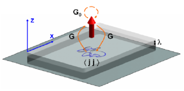
Figure 1: (color online) Schematic geometrical setup. A plane metallic or superconducting slab lies parallel to the $(x,y)$ plane. The atom with magnetic moment $\bm{\mu}$ indicted by the arrow, is located in vacuum at a distance $z$ from the surface. The atom suffers spontaneous or thermally stimulated magnetic spin-flip transitions, as indicated by $\bm{G}_{0}$ and $\bm{G}$, thereby becoming more weakly trapped and eventually lost. Johnson current noise $\langle\mathbf{j}\mathbf{j}\rangle$ within the penetration depth $\lambda$ contributes to magnetic-field fluctuations at the position of the atom.

We turn now to the spin flip rate for an atom located in vacuum near a superconducting slab, as illustrated in Fig. 1. Following Refs. Rekdal et al. (2004); Scheel et al. (2005); Skagerstam et al. (2006), we consider a ground-state alkali atom, magnetically trapped in a weak-field-seeking Zeeman sub-level. The noise in the magnetic field, due both to vacuum fluctuations and to thermal currents in the surface, induces transitions between the levels, making the atomic spin change direction (spin flip) and ultimately causing the atom to be lost from the microtrap.

As briefly outlined in Appendix A, the spin-flip lifetime of an atom at position $\bm{r}_{A}$ is directly related to the imaginary part of the dyadic Green tensor $\bm{G}(\mathbf{r}_{A},\mathbf{r}_{A},\omega)$ of Maxwell’s theory. The usual, free-space spontaneous emission rate is determined by the vacuum contribution $\bm{G}_{0}$. For a typical transition frequency of $f_{A}=\omega_{A}/(2\pi)=500$ kHz, corresponding to an energy of approximately 2 neV, this natural lifetime at zero temperature is $\tau_{0}\approx 2\times 10^{25}$ seconds Scheel et al. (2005), which can safely be considered infinite. The dominant contribution to the lifetime reduction comes from the magnetic-field fluctuations induced by the Johnson-Nyquist noise in the dielectric body. As shown in Fig. 1 and discussed in the Appendix, the current noise translates through the Green tensors to a magnetic-field fluctuation at the position of the atom.

For a thick superconducting slab described by an optical conductivity in the limit $\sigma^{\prime\prime}(\omega)\gg\sigma^{\prime}(\omega)$ and in the near field regime $\lambda_{L}\ll z\ll 2\pi/k$ one calculates, using the results of Ref. Skagerstam et al. (2006), a spin-flip rate of

$$\Gamma\equiv\frac{1}{\tau_{A}}\approx\Gamma_{0}\left(\bar{n}_{\rm th}+1\right)\left[1+\frac{27}{64(\omega\mu_{0})^{1/2}k^{3}z^{4}}\frac{\sigma^{\prime}}{(\sigma^{\prime\prime})^{3/2}}\right]\,.$$ (13)

Here $\tau_{A}$ is the spin flip lifetime, $\Gamma_{0}$ is the free-space decay rate, $\bar{n}_{\rm th}$ is the mean thermal photon number at the transition frequency $\omega_{A}$, $k=\omega_{A}/c$, and $z$ is the atom-superconductor distance. In the following sections we investigate the consequences for this rate of using the expressions for the optical conductivity $\sigma(\omega)=\sigma^{\prime}(\omega)+i\sigma^{\prime\prime}(\omega)$ obtained from a two-fluid description, from BCS theory and from Eliashberg theory.

III.1 Two-fluid model

To estimate the order of magnitude of these parameters, we first consider the simple two-fluid model. Using the expression (3) for the optical conductivity, Eq. (13) reduces to the expression Skagerstam et al. (2006)

$$\Gamma\equiv\frac{1}{\tau_{A}}\approx\Gamma_{0}\left(\bar{n}_{\rm th}+1\right)\left[1+2\left(\frac{3}{4}\right)^{3}\frac{1}{k^{3}\delta^{2}}\frac{\lambda_{L}^{3}}{z^{4}}\right]\,.$$ (14)

We take Nb as a representative superconducting material throughout. Table 1 shows a few values reported in the literature for the conductivity $\sigma_{0}$ of the normal state. We note that the ultra-pure niobium sample of Ref. Casalbuoni et al. (2005) has a hundred times higher conductivity than the films of Refs. Perkowitz et al. (1985); Pronin et al. (1998). Through the simple Drude model Ashcroft and Mermin (1976)

$$\sigma_{0}=\varepsilon_{0}\omega_{p}^{2}\tau\,,$$ (15)

we can relate $\sigma_{0}$ to an electron lifetime $\tau=1/\gamma$ due to elastic scattering at impurities or defects. $\hbar\omega_{p}$ is the bulk plasmon energy, which we set equal to 10 eV Ashcroft and Mermin (1976); Perkowitz et al. (1985). The corresponding $\tau$ values are given in the last column of Table 1. With an atomic transition frequency of 500 kHz, we obtain for the ultrapure sample a normal-state skin depth of $\delta_{0}=\sqrt{2/(\mu_{0}\omega\sigma_{0})}\approx 16$ $\mu$m and a value approximately ten times larger for the films.

Table 1: Normal-state conductivity $\sigma_{0}$ measured on several different samples of niobium. The approximate scattering times $\tau$ are obtained from the Drude model (15). The corresponding plasma frequency is $\omega_{p}\approx 10\,\mbox{eV}/\hbar\simeq 1.5\times 10^{16}\mbox{s}^{-1}$.

Reference	$\sigma_{0}$ ($\mu\Omega^{-1}{\rm cm}^{-1}$)	$\tau$ (fs)
Perkowitz et al. Perkowitz et al. (1985)	0.2	10
Pronin et al. Pronin et al. (1998)	0.25	13
Klein et al. Klein et al. (1984)	0.85	43
Casalbuoni et al. Casalbuoni et al. (2005)	20	1000

A rough estimate for the penetration depth of the superconductor at zero temperature is given by

$$\lambda_{L}=\left(\frac{\Lambda}{\mu_{0}}\right)^{\frac{1}{2}}\approx\left(\frac{1}{\mu_{0}\,\varepsilon_{0}\,\omega_{p}^{2}}\right)^{\frac{1}{2}}=\frac{c}{\omega_{p}}\approx 20\,\mbox{nm}\,,$$ (16)

where we have assumed that all electrons move freely. This simple estimate is comparable to the BCS value of 35 nm Miller (1959), and to the experimental values of 46 nm for the ultrapure sample Casalbuoni et al. (2005) and 90 nm for the niobium film in Pronin et al. (1998).

III.2 BCS versus Eliashberg theory

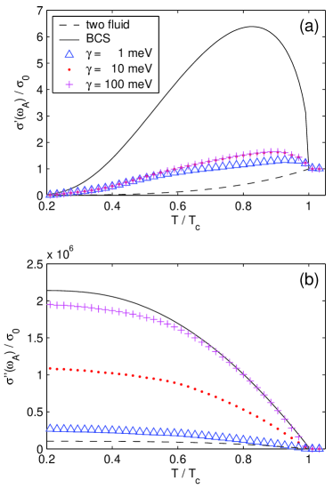
Figure 2: (color online) Temperature dependence of (a) real part $\sigma^{\prime}(\omega_{A})$ and (b) imaginary part $\sigma^{\prime\prime}(\omega_{A})$ of the optical conductivity, normalised to the normal state conductivity $\sigma_{0}$. $\omega_{A}=2\pi\times 500\mbox{kHz}$ is the atomic spin-flip frequency, $T_{c}=9.2$ K is the superconductor transition temperature. The different lines correspond to the results for the two-fluid model (dashed line), using $\delta_{0}=16$ $\mu$m and $\lambda_{L}(0)=35$ nm, BCS theory (solid line), and Eliashberg theory (symbols) for three elastic impurity scattering rates $\gamma$.

.

Now we discuss how the two-fluid estimates are modified within the framework of BCS and Eliashberg theories. For the BCS theory of niobium we use a zero-temperature gap parameter of $\Delta=1.4$ meV, corresponding to a transition temperature of $T_{c}=9.2$ K, and a Debye temperature of $\hbar\omega_{D}/k_{B}=275$ K, and we compute the optical conductivity by means of the Mattis–Bardeen formulas in the dirty limit Mattis and Bardeen (1958).

For the implementation of the Eliashberg equations, we have considered an $\alpha^{2}F(\omega)$ function calculated using linear response theory Baroni et al. (2001) and norm-conserving pseudopotentials. The electron-phonon matrix elements were calculated on a 32³ wavevector grid for both electrons and phonons. Our result (not shown) is similar to that presented in Ref. Savrasov and Savrasov (1996), though with spectral features that are less pronounced, in better agreement with the data of tunneling experiments. As far as the calculated atomic spin flip rates are concerned, we do not find any significant difference between these two $\alpha^{2}F(\omega)$ functions.

Figure 2 shows results for the (a) real and (b) imaginary part of the optical conductivity versus temperature $T$. The solid lines show the results from BCS theory in the dirty limit, the dashed lines are for the two-fluid model and the symbol series are for Eliashberg theory with various values of the elastic impurity scattering rate $\gamma$. In Fig. 2(a), the $\sigma^{\prime}(\omega_{A})$ obtained from the two-fluid model decreases monotonically with temperature because of the decrease in the normal density $n_{n}(T)$, whereas the BCS and Eliashberg curves show an enhancement of $\sigma^{\prime}(\omega_{A})$ at temperatures immediately below the transition temperature $T_{c}$. This is due to the coherence peak, which forms as a consequence of the modified quasiparticle dispersion in the superconducting state. The peak is most pronounced within the BCS framework in the dirty limit. As we move away from the dirty limit towards a clean superconductor, using the Eliashberg theory with decreasing rates $\gamma$, we observe that the peak gradually disappears, in agreement with Marsiglio et al. (1994). Thus the Eliashberg theory interpolates between the two extreme cases of the two-fluid model and the dirty limit of BCS theory by varying the chosen value of $\gamma$.

In Fig. 2(b) we show the imaginary part of the optical conductivity. Again, the BCS result is according to the theory of Mattis and Bardeen Mattis and Bardeen (1958) for a dirty superconductor. Here too, we see that the Eliashberg theory with variable $\gamma$ provides a link between the two-fluid and BCS extremes. In the low frequency limit, the BCS result takes the analytical form

$$\sigma_{\rm BCS}^{\prime\prime}(\omega)=\sigma_{0}\,\frac{\pi\Delta}{\hbar\omega}\,\tanh\frac{\Delta}{2k_{B}T}\,,$$ (17)

where $\Delta$ is the temperature-dependent gap parameter. We note that this $1/\omega$ dependence of $\sigma^{\prime\prime}$ is the same in all three models. This is a consequence of the Kramers-Kronig relations together with the fact that $\sigma^{\prime}$ has a $\delta$ singularity at $\omega=0$ associated with the response of the superfluid to a dc field.

We are using here a theory in which the material responds locally to a field. Although this is not strictly so, nonlocality can be incorporated empirically into the theory of the superconductor through a modified penetration depth Skagerstam et al. (2006). The effect of nonlocality on the atom-surface response is negligible since the penetration depth is small compared with the atom-superconductor distance.

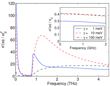
Figure 3: (color online) $\sigma^{\prime}(\omega)$ at 4.2 K as a function of frequency for three elastic scattering rates $\gamma$, as computed within the framework of Eliashberg theory. The peak at zero frequency is attributed to the condensate, and the peak at 1 THz to the breaking of Cooper pairs. In the inset we show that the condensate peak saturates at low frequencies.

As discussed in Sec.II.2.2, the BCS coherence peak illustrated by the solid line in Fig. 2(a) increases with decreasing frequency, diverging as $\omega\to 0$. This behaviour is greatly suppressed when inelastic phonon scattering is taken into account using Eliashberg theory (see also the discussion in Sec. II.4), as plotted in Fig. 3. This figure shows the real part of the optical conductivity $\sigma^{\prime}(\omega)$ at 4.2 K with three values of $\gamma$, spanning the $10-1000\,$ps range of scattering times given in Table 1. The peak in Figure 3 at 1 THz is the conductivity associated with the breakup of Cooper pairs. The lower-frequency peak, which is the one of relevance here, no longer diverges at low frequency but reaches a constant value, shown inset in the figure for frequencies below 2 GHz. Here, as in Fig. 2, the value of $\sigma^{\prime}$ is normalised to the normal state conductivity to remove most of the dependence on $\gamma$. Since the atomic spin flip frequency is bound to be in this low frequency range, the Eliashberg results shown in Fig. 2 apply to all cases of experimental interest. We recall that the $\sigma^{\prime}$ of the two fluid model in Eq. (3) is also frequency independent.

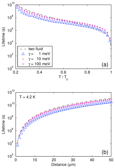
Figure 4: (color online) Spin-flip lifetime $\tau_{A}$ of a trapped atom near a superconducting slab as a function of (a) temperature (for 10 $\mu$m atom-surface distance), and (b) distance (at 4.2 K). The smallest distance in (b) is 1 $\mu$m (with $\tau_{A}\approx 5000$ s for $\gamma=1$ meV). For the calculation of $\tau_{A}$ we use Eq. (13) and the optical conductivity computed within Eliashberg theory for different elastic scattering rates $\gamma$. The atomic transition frequency is fixed at 500 kHz throughout. The dashed lines correspond to calculations performed with the two-fluid model and the parameters given in Ref. Skagerstam et al. (2006) (London length $\lambda_{L}=35$ nm).

Finally, in Fig. 4(a) we show the spin-flip lifetime $\tau_{A}=1/\Gamma$ [see Eq. (13)] as a function of temperature for an atom-surface distance of 10 $\mu$m. The dashed line indicates the results obtained from the two-fluid model of Ref. Skagerstam et al. (2006). The lifetimes obtained from Eliashberg theory (symbols) are smaller, but only by a factor of ten or less: the influence of elastic scattering rates $\gamma$ on the spin-flip lifetime is not very strong. This indicates that the quality of the niobium is not critical. Surprisingly, we find that $\tau_{A}$ is smallest for the high-quality sample with $\gamma=1$ meV, highest for the intermediate value $\gamma=10$ meV, and falls off again slightly for $\gamma=100$ meV. In Fig. 4(b) we show $\tau_{A}$ as a function of atom-surface distance at 4.2 K (T/T${}_{c}=0.46$).

For an atom-surface distance of 1 $\mu$m we obtain for $\gamma=1$ meV a lifetime $\tau_{A}\approx 5000$ seconds at a transition frequency of $\omega_{A}/2\pi=500\,\mbox{kHz}$. Values for other distances can be obtained directly from the $z^{4}$ scaling of our central equation, Eq. (13). For other (low) frequencies, the lifetime given by Eq. (13) scales approximately as $\omega_{A}^{2}$. This follows from the frequency independence of $\sigma^{\prime}$ for $\omega>0$ and the $1/\omega$ dependence of $\sigma^{\prime\prime}$.

IV Summary

In this article, we have resolved the controversy surrounding the appropriate use of model assumptions for the electromagnetic energy dissipation in superconducting materials. We have discussed the three most common models of superconductivity, the two-fluid model, BCS and Eliashberg theories, in ascending order of sophistication. The spin flip lifetime of neutral atoms trapped near a superconducting niobium surface is predicted to be much shorter when treated in the BCS theory than it is in the two fluid model. However, Eliashberg theory, which improves upon the BCS theory by including the finite quasiparticle lifetime, predicts only slightly shorter lifetimes.

The Eliashberg theory interpolates between the two-fluid model and the BCS theory. For intermediate scattering rates, corresponding to real samples, the simple two-fluid model gives remarkably accurate estimates of the Eliashberg results. We have found that the lifetime depends only little on the precise value of the impurity scattering rate $\gamma$.

Our numerical results based on the Eliashberg theory show that the expected spin-flip lifetime for an atom placed one micrometer away from a $4.2$ K superconducting planar niobium surface exceeds several thousand seconds at an atomic transition frequency of $500$ kHz. This is expected to scale roughly as $\omega_{A}^{2}$ and $z^{4}$. Hence, superconducting surfaces provide an extremely low-noise environment for magnetically trapped neutral atoms and thus have great potential for coherent manipulation of atoms.

Appendix A Spin flip lifetime

In this appendix we sketch briefly how to derive our basic expression (13). The derivation follows closely the general framework of Refs. Henkel et al. (1999); Rekdal et al. (2004). There is, however, a subtle point regarding the fluctuation-dissipation theorem, which we shall partly rephrase in the language of solid-state physics. In the general framework developed by Welsch and coworkers Scheel et al. (1998); Vogel and Welsch (2006); Raabe et al. (2007) one introduces Langevin noise operators with bosonic commutation relations, in order to fulfil the linear fluctuation-dissipation theorem. However, for calculating expectation values of bilinear operator products as in case of the spin-flip lifetime, there is no particular need for such an approach.

We consider an atom located in the vicinity of a dielectric body, as depicted in Fig. 1, which is in a given magnetic sublevel. The coupling to the magnetic-field fluctuations is described through a Zeeman interaction Hamiltonian in the rotating wave approximation. For a low-field seeking atom, the spin flip transition is associated with an emission process, and the transition rate is simply given by Fermi’s golden rule Henkel et al. (1999); Fortagh and Zimmermann (2007)

$$\Gamma=\sum\limits_{\alpha,\beta}\frac{\langle i|\mu_{\alpha}|f\rangle\langle f|\mu_{\beta}|i\rangle}{\hbar^{2}}\,\left<B_{\alpha}^{\phantom{\dagger}}(\mathbf{r}_{A},\omega_{A})B_{\beta}^{\dagger}(\mathbf{r}_{A},\omega_{A})\right>\,.$$ (18)

Here $\alpha$ and $\beta$ denote the Cartesian components, $i$ and $f$ are the initial and final state of the scattering process, respectively, $\mathbf{\mu}$ is the magnetic moment operator, and $\mathbf{B}(\mathbf{r}_{A},\omega)$ the Fourier transform of the magnetic field component with positive frequency. The position of the atom is $\mathbf{r}_{A}$ and $\omega_{A}$ is the transition frequency.

Now we relate the spectral density of the magnetic field to the current noise in the dielectric. In linear response theory we can use the Green tensor $\bm{G}$ of Maxwell’s theory to relate the current $\mathbf{j}$ to the magnetic field $\mathbf{B}$ according to Vogel and Welsch (2006); Rekdal et al. (2004)

$$\mathbf{B}(\mathbf{r},\omega)=\mu_{0}\int d^{3}r^{\prime}\,\bm{\nabla}\times\bm{G}(\mathbf{r},\mathbf{r}^{\prime},\omega)\,\mathbf{j}(\mathbf{r}^{\prime},\omega)\,,$$ (19)

with a corresponding equation for $\mathbf{B}^{\dagger}(\mathbf{r},\omega)$. Thus, the spectral density of the magnetic-field fluctuations is given by convolving the spectral density $\langle j_{\alpha}(\mathbf{r},\omega)j_{\beta}^{\dagger}(\mathbf{r}^{\prime},\omega)\rangle$ of the current fluctuations with Maxwell’s Green tensors, which describe how the field produced by the current fluctuation propagates to the position $\mathbf{r}_{A}$ of the atom (see Fig. 1). In the following we consider for simplicity only isotropic and local dielectric media.

The calculation of $\langle j(\omega)j^{\dagger}(\omega)\rangle$ is a common problem in solid state physics Mahan (1981). For instance, in our present approach $j$ could be the normal current $j_{n}$ or the super current $j_{s}$ of the superconductor. To express the spectral density of current correlations in terms of the optical conductivity, we first note that $\sigma^{\prime}(\omega)$ is related to the retarded current-current correlation via $\omega\sigma^{\prime}(\omega)=\Re e\int_{0}^{\infty}dt\,e^{i\omega t}\left<[j(t),j^{\dagger}(0)]\right>$, which is a general result of linear-response theory Kubo et al. (1985). A common link between the ordered and retarded current-current correlation is provided by the spectral function $\rho(t)=\left<[j(t),j^{\dagger}(0)]\right>$. Its Fourier transform can be obtained upon insertion of a complete set of states $|m\rangle$ with energy $E_{m}$ Mahan (1981)

$$\rho(\omega) = \left(1-e^{-\beta\hbar\omega}\right)Z^{-1}\sum_{m,n}e^{-\beta E_{m}}\left|\langle m|j|n\rangle\right|^{2}$$ (20)

$$\qquad\times 2\pi\delta(\omega-(E_{n}-E_{m})/\hbar)\,,$$

with $Z$ being the partition function. From Eq. (20) one immediately obtains $\langle j(\omega)j^{\dagger}(\omega)\rangle=\rho(\omega)/(1-e^{-\beta\hbar\omega})$. The relation between the retarded current-current correlation and the spectral density is given through the Lehmann representation as $\rho(\omega)=2\omega\sigma^{\prime}(\omega)$ Mahan (1981). Thus, the desired relation between $\langle j(\omega)j^{\dagger}(\omega)\rangle$ and the optical conductivity reads

$$\langle j(\omega)j^{\dagger}(\omega)\rangle=\bigl{[}\bar{n}_{\rm th}(\hbar\omega)+1\bigr{]}\,2\omega\,\sigma^{\prime}(\omega)\,.$$ (21)

One finally uses the expression $\Im m\,\bm{G}=(\mu_{0}/\omega)\,\bm{G}\sigma^{\prime}\bm{G}^{*}$, which follows directly from Maxwell’s equations Henry and Kazarinov (1996); Scheel et al. (1998), to relate the scattering rate (18) to the imaginary part of the Green tensor. The final equation (13) is obtained according to the prescription given in Ref. Skagerstam et al. (2006).

References

- Hinds and Hughes (1999) E. A. Hinds and I. A. Hughes, J. Phys. D 32, R119 (1999).
- Folman et al. (2002) R. Folman, P. Krüger, J. Schmiedmayer, J. Denschlag, and C. Henkel, Adv. in Atom. Mol. and Opt. Phys. 48, 263 (2002).
- (3) C. Henkel, J. Schmiedmayer, and C. Westbrook, Euro. Phys. J. D 35, 1 (2006) and following articles.
- Fortagh and Zimmermann (2007) J. Fortagh and C. Zimmermann, Rev. Mod. Phys. 79, 235 (2007).
- Hänsel et al. (2001) W. Hänsel, J. Reichel, P. Hommelhoff, and T. W. Hänsch, Phys. Rev. A 64, 063607 (2001).
- Hinds et al. (2001) E. A. Hinds, C. J. Vale, and M. G. Boshier, Phys. Rev. Lett. 86, 1462 (2001).
- Andersson et al. (2002) E. Andersson, T. Calarco, R. Folman, M. Andersson, B. Hessmo, and J. Schmiedmayer, Phys. Rev. Lett. 88, 100401 (2002).
- Wang et al. (2005) Y.-J. Wang, D. Z. Anderson, V. M. Bright, E. A. Cornell, Q. Diot, T. Kishimoto, M. Prentiss, R. A. Saravanan, S. R. Segal, and S. Wu, Phys. Rev. Lett. 94, 090405 (2005).
- Schumm et al. (2005) T. Schumm, S. Hofferberth, L. M. Andersson, S. Wildermuth, S. Groth, I. Bar-Joseph, J. Schmiedmayer, and P. Krüger, Nature Phys. 1, 57 (2005).
- Jo et al. (2007) G.-B. Jo, Y. Shin, S. Will, T. A. Pasquini, M. Saba, W. Ketterle, D. E. Pritchard, M. Vengalattore, and M. Prentiss, Phys. Rev. Lett. 98, 030407 (2007).
- Calarco et al. (2000) T. Calarco, E. A. Hinds, D. Jaksch, J. Schmiedmayer, J. I. Cirac, and P. Zoller, Phys. Rev. A 61, 022304 (2000).
- Charron et al. (2006) E. Charron, M. Cirone, A. Negretti, J. Schmiedmayer, and T. Calarco, Phys. Rev. A 74, 012308 (2006).
- Treutlein et al. (2006) P. Treutlein, T. W. Hänsch, J. Reichel, A. Negretti, M. A. Cirone, and T. Calarco, Phys. Rev. A 74, 022312 (2006).
- Hohenester et al. (2007) U. Hohenester, P. K. Rekdal, A. Borzi, and J. Schmiedmayer, Phys. Rev. A 75, 023602 (2007).
- Paul et al. (2005) T. Paul, K. Richter, and P. Schlagheck, Phys. Rev. Lett. 94, 020404 (2005).
- Wildermuth et al. (2005) S. Wildermuth, S. Hofferberth, I. Lesanovsky, E. Haller, L. Mauritz-Andersson, S. Groth, I. Bar-Joseph, P. Krüger, and J. Schmiedmayer, Nature (London) 435, 440 (2005).
- Scheel et al. (2007) S. Scheel, R. Fermani, and E. A. Hinds, Phys. Rev. A 75, 064901 (2007).
- Jones et al. (2003) M. P. A. Jones, C. J. Vale, D. Sahagun, B. V. Hall, and E. A. Hinds, Phys. Rev. Lett. 91, 080401 (2003).
- Lin et al. (2004) Y. Lin, I. Teper, C. Chin, and V. Vuletic, Phys. Rev. Lett. 92, 050404 (2004).
- Henkel et al. (1999) C. Henkel, S. Pötting, and M. Wilkens, Appl. Phys. B 69, 379 (1999).
- Rekdal et al. (2004) P. K. Rekdal, S. Scheel, P. L. Knight, and E. A. Hinds, Phys. Rev. A 70, 013811 (2004).
- Scheel et al. (2005) S. Scheel, P. K. Rekdal, P. L. Knight, and E. A. Hinds, Phys. Rev. A 72, 042901 (2005).
- Nirrengarten et al. (2006) T. Nirrengarten, A. Qarry, C. Roux, A. Emmert, G. Nogues, M. Brune, J. M. Raimond, and S. Haroche, Phys. Rev. Lett. 97, 200405 (2006).
- Mukai et al. (2007) T. Mukai, C. Hufnagel, A. Kasper, T. Meno, A. Tsukada, K. Semba, and F. Shimizu, Phys. Rev. Lett. 98, 260407 (2007).
- Skagerstam et al. (2006) B. S. Skagerstam, U. Hohenester, A. Eiguren, and P. K. Rekdal, Phys. Rev. Lett. 97, 070401 (2006).
- (26) S. Scheel, E. A. Hinds, and P. L. Knight, arXiv:quant-ph/0610095.
- (27) B. S. Skagerstam, U. Hohenester, A. Eiguren, and P. K. Rekdal, arXiv:quant-ph/061025.
- Bardeen et al. (1957) J. Bardeen, L. N. Cooper, and J. R. Schrieffer, Phys. Rev. 108, 1175 (1957).
- Eliashberg (1960) G. M. Eliashberg, Soviet. Phys. JETP 11, 696 (1960).
- Marsiglio and Carbotte (2002) F. Marsiglio and J. P. Carbotte, The Physics of Superconductors (Springer, Berlin, 2002), p. 233.
- Rickayzen (1965) G. Rickayzen, Theory of Superconductivity (Interscience, New York, 1965).
- Tinkham (1975) M. Tinkham, Introduction to Superconductivity (McGraw-Hill, New York, 1975).
- Mahan (1981) G. D. Mahan, Many-Particle Physics (Plenum, New York, 1981).
- London and London (1935) F. London and H. London, Proc. Roy. Soc. Lond. 133, 497 (1935).
- Gorter and Casimir (1934) C. S. Gorter and H. Casimir, Z. Phys. 35, 963 (1934).
- Hebel and Slichter (1959) L. C. Hebel and C. P. Slichter, Phys. Rev. 113, 1504 (1959).
- Fröhlich (1950) H. Fröhlich, Phys. Rev. 79, 845 (1950).
- Cooper (1956) L. N. Cooper, Phys. Rev. 104, 1189 (1956).
- Mattis and Bardeen (1958) D. C. Mattis and J. Bardeen, Phys. Rev. 111, 412 (1958).
- Klein et al. (1984) O. Klein, E. J. Nicol, K. Holczer, and G. Grüner, Phys. Rev. B 50, 6307 (1984).
- Marsiglio et al. (1988) F. Marsiglio, M. Schossmann, and J. P. Carbotte, Phys. Rev. B 37, 4965 (1988).
- Carbotte (1990) J. P. Carbotte, Rev. Mod. Phys. 62, 1027 (1990).
- Nicol and Carbotte (1992) E. J. Nicol and J. P. Carbotte, Phys. Rev. B 45, 10519 (1992).
- (44) S. B. Nam, Phys. Rev. 156, 470 (1967); ibid. 156, 487 (1967).
- Anderson (1959) P. W. Anderson, J. Phys. Chem- Solids 11, 26 (1959).
- Balatsky et al. (2006) A. V. Balatsky, I. Vekhter, and J. X. Zhu, Rev. Mod. Phys. 78, 373 (2006).
- Casalbuoni et al. (2005) S. Casalbuoni, E. A. Knabbe, J. Kötzler, L. Lilje, L. von Sawiliski, P. Schmüser, and B. Steffen, Nucl. Instrum. Meth. Phys. Res. A 538, 45 (2005).
- Perkowitz et al. (1985) S. Perkowitz, G. L. Carr, B. Subramaniam, and B. Mitrovic, Phys. Rev. B 32, 153 (1985).
- Pronin et al. (1998) A. V. Pronin, M. Dressel, A. Pimenov, A. Loidl, I. V. Roshchin, and L. H. Greene, Phys. Rev. B 57, 14416 (1998).
- Ashcroft and Mermin (1976) N. W. Ashcroft and N. D. Mermin, Solid State Physics (Saunders, Fort Worth, 1976).
- Miller (1959) P. B. Miller, Phys. Rev. 113, 1209 (1959).
- Baroni et al. (2001) S. Baroni, S. de Gironcoli, A. Dal Corso, and P. Giannozzi, Rev. Mod. Phys. 73, 515 (2001).
- Savrasov and Savrasov (1996) S. Y. Savrasov and D. Y. Savrasov, Phys. Rev. B 54, 16487 (1996).
- Marsiglio et al. (1994) F. Marsiglio, J. P. Carbotte, R. Akis, D. Achkir, and M. Poirier, Phys. Rev. B 50, 7203 (1994).
- Scheel et al. (1998) S. Scheel, L. Knöll, and D.-G. Welsch, Phys. Rev. A 58, 700 (1998).
- Vogel and Welsch (2006) W. Vogel and D.-G. Welsch, Quantum Optics (Wiley, Berlin, 2006).
- Raabe et al. (2007) C. Raabe, S. Scheel, and D. G. Welsch, Phys. Rev. A 75, 053813 (2007).
- Kubo et al. (1985) R. Kubo, M. Toda, and M. Hashitsume, Statistical Physics II (Springer, Berlin, 1985).
- Henry and Kazarinov (1996) C. H. Henry and R. F. Kazarinov, Rev. Mod. Phys. 68, 801 (1996).