Three-Port Beam Splitters/Combiners for Interferometer Applications

R. Schnabel, A. Bunkowski, O. Burmeister, and K. Danzmann

Max-Planck-Institut für Gravitationsphysik (Albert-Einstein-Institut), Universität Hannover,
Callinstr. 38, 30167 Hannover, Germany

Abstract

We derive generic phase and amplitude coupling relations for beam splitters/combiners that couple a single port with three output ports or input ports, respectively. We apply the coupling relations to a reflection grating that serves as a coupler to a single-ended Fabry-Perot ring cavity. In the impedance matched case such an interferometer can act as an all-reflective ring mode-cleaner. It is further shown that in the highly under-coupled case almost complete separation of carrier power and phase signal from a cavity strain can be achieved.

OCIS codes:  050.1950, 120.3180, 230.1360.

Two-port beam splitters/combiners, for example the partially transmitting mirror, are key devices in laser interferometry. They serve as 50/50 beam splitters in Michelson interferometers and as low transmission couplers to cavities. Amplitude and phase relations of two-port beam splitters/combiners are well-known. In the case of grating optics, diffraction orders of a greater number can couple to one input port. Recently, a reflection grating with three diffraction orders was used for interferometer purposes; laser light was coupled into a linear high finesse Fabry-Perot cavity using the second-order Littrow configuration [1]. The grating was built from a binary structure. This property together with the second-order Littrow configuration provided a symmetry against the grating’s normal. The system was theoretically analyzed in [2]. It was shown that the new three-port (3p) coupled Fabry-Perot interferometer can be designed such that resonating carrier light is completely back-reflected towards the laser source. The additional interferometer port is then on a dark fringe and contains half of the interferometer strain signal.

In this letter we first derive the generic coupling relations of three-port (3p) beam splitters. This includes coupling amplitudes as well as coupling phases which are required for interferometric applications. Our description includes arbitrary gratings with three orders of diffraction regardless of the groove shape and the diffraction angles, as shown in Fig. 1. We then investigate the three-port reflection grating coupled Fabry-Perot ring interferometer and show that for a resonating carrier a dark port can be constructed that contains an arbitrary high fraction of the interferometer’s strain signal.

Fig. 1: Two examples of three-port (3p) beam splitters/combiners. Input fields $a_{i}$ and output fields $b_{i}$ denote complex amplitudes of the electric field. a) Asymmetric triangular grating in second order Littrow configuration. b) Binary grating in non-Littrow configuration.

Optical devices can be described by a scattering matrix formalism [3]. In general the coupling of $n$ input and $n$ output ports require an $n\times n$ scattering matrix S. The $n$ complex amplitudes of incoming and outgoing fields are combined into vectors a and b, respectively. For a loss-less device S has to be unitary to preserve energy, and reciprocity demands $|S_{ij}|\equiv|S_{ji}|$ for all elements $S_{ij}$ of S. For a generic three-port device 6 coupling amplitudes and 9 coupling phases are involved. Since 3 input and 3 output fields are considered the number of phases can be reduced to 6 without loss of physical generality; the remaining 6 phases describe the phases of the 6 fields with respect to a local oscillator field. Here we choose the phases such that the matrix S is symmetric, and $\textbf{b}=\textbf{S}\times\textbf{a}$ can therefore be written as

$$\left(\begin{array}[]{c}b_{1}\\ b_{2}\\ b_{3}\\ \end{array}\right)=\left(\begin{array}[]{cll}\eta_{1}e^{i\phi_{1}}&\eta_{4}e^{i\phi_{4}}&\eta_{5}e^{i\phi_{5}}\!\!\\ \eta_{4}e^{i\phi_{4}}&\eta_{2}e^{i\phi_{2}}&\eta_{6}e^{i\phi_{6}}\!\!\\ \eta_{5}e^{i\phi_{5}}&\eta_{6}e^{i\phi_{6}}&\eta_{3}e^{i\phi_{3}}\!\!\\ \end{array}\right)\!\times\!\left(\begin{array}[]{c}a_{1}\\ a_{2}\\ a_{3}\\ \end{array}\right)\,,$$ (1)

where $0<\eta_{i}<1$ for all $i$ describes the amplitude and $e^{i\phi_{i}}$ the phase of coupling. Fig. 1 shows two examples of three-port devices. In both cases the input beam splits into three beams, and vice versa three input beams can interfere into a single one. However, one realizes that the rigorously defined scattering matrix for the device in Fig. 1b) has dimension $6\times 6$; but this matrix contains null elements because not 6 but only 3 ports couple and the matrix can be reduced to the matrix as given in Eq. (1).

The unitarity condition $\textbf{S}^{\dagger}\textbf{S}=\textbf{1}$ entails the following set of equations:

$$1 \!\!=\!\! \eta_{1}^{2}+\eta_{4}^{2}+\eta_{5}^{2}\,,\;$$ (2)

$$1 \!\!=\!\! \eta_{2}^{2}+\eta_{4}^{2}+\eta_{6}^{2}\,,\;$$ (3)

$$1 \!\!=\!\! \eta_{3}^{2}+\eta_{5}^{2}+\eta_{6}^{2}\,,\;$$ (4)

$$|\mbox{cos}(2\phi_{4}\!-\!\phi_{1}\!-\!\phi_{2})| \!\!=\!\! \frac{|\eta_{5}^{2}\eta_{6}^{2}-\eta_{1}^{2}\eta_{4}^{2}-\eta_{2}^{2}\eta_{4}^{2}|}{2\eta_{4}^{2}\eta_{1}\eta_{2}}\,,\;$$ (5)

$$|\mbox{cos}(2\phi_{5}\!-\!\phi_{1}\!-\!\phi_{3})| \!\!=\!\! \frac{|\eta_{4}^{2}\eta_{6}^{2}-\eta_{1}^{2}\eta_{5}^{2}-\eta_{3}^{2}\eta_{5}^{2}|}{2\eta_{5}^{2}\eta_{1}\eta_{3}}\,,\;$$ (6)

$$|\mbox{cos}(2\phi_{6}\!-\!\phi_{2}\!-\!\phi_{3})| \!\!=\!\! \frac{|\eta_{4}^{2}\eta_{5}^{2}-\eta_{2}^{2}\eta_{6}^{2}-\eta_{3}^{2}\eta_{6}^{2}|}{2\eta_{6}^{2}\eta_{2}\eta_{3}}\,,\;$$ (7)

$$|\mbox{cos}(\phi_{6}\!+\!\phi_{4}\!-\!\phi_{5}\!-\!\phi_{2})| \!\!=\!\! \frac{|\eta_{1}^{2}\eta_{4}^{2}-\eta_{2}^{2}\eta_{4}^{2}-\eta_{5}^{2}\eta_{6}^{2}|}{2\eta_{2}\eta_{4}\eta_{5}\eta_{6}}\,,\;$$ (8)

$$|\mbox{cos}(\phi_{6}\!-\!\phi_{4}\!-\!\phi_{5}\!+\!\phi_{1})| \!\!=\!\! \frac{|\eta_{3}^{2}\eta_{5}^{2}-\eta_{1}^{2}\eta_{5}^{2}-\eta_{4}^{2}\eta_{6}^{2}|}{2\eta_{1}\eta_{4}\eta_{5}\eta_{6}}\,,\;\;$$ (9)

$$|\mbox{cos}(\phi_{6}\!-\!\phi_{4}\!+\!\phi_{5}\!-\!\phi_{3})| \!\!=\!\! \frac{|\eta_{2}^{2}\eta_{6}^{2}-\eta_{4}^{2}\eta_{5}^{2}-\eta_{3}^{2}\eta_{6}^{2}|}{2\eta_{3}\eta_{4}\eta_{5}\eta_{6}}\,.\;\;\;\;\;\;$$ (10)

Eqs. (2)-(10) set boundaries for physically possible coupling amplitudes and phases of the generic loss-less 3p beam splitter/combiner. The first three equations represent the energy conservation law and arise from the diagonal elements of the unitarity condition. The next six equations arise from the off-diagonal elements. They are already simplified to contain just a single cosine term. However, it can be easily deduced that up to three phases in the scattering matrix S can be chosen arbitrarily. In this analysis we choose the phases $\phi_{1},\phi_{2},\phi_{3}$ to be zero. This is a permitted choice without introducing any restriction on possible coupling amplitudes. Then the phases of the scattering matrix can be written as

$$\phi_{1} = \phi_{2}\;\;=\;\;\phi_{3}\;\;=\;\;0\,,$$

$$\phi_{4} = -\frac{1}{2}\mbox{arccos}\left(\frac{\eta_{1}^{2}\eta_{4}^{2}+\eta_{2}^{2}\eta_{4}^{2}-\eta_{5}^{2}\eta_{6}^{2}}{2\eta_{4}^{2}\eta_{1}\eta_{2}}\right)-\frac{\pi}{2}\,,$$

$$\phi_{5} = \frac{1}{2}\mbox{arccos}\left(\frac{\eta_{4}^{2}\eta_{6}^{2}-\eta_{1}^{2}\eta_{5}^{2}-\eta_{3}^{2}\eta_{5}^{2}}{2\eta_{5}^{2}\eta_{1}\eta_{3}}\right)\,,$$ (11)

$$\phi_{6} = -\frac{1}{2}\mbox{arccos}\left(\frac{\eta_{2}^{2}\eta_{6}^{2}+\eta_{3}^{2}\eta_{6}^{2}-\eta_{4}^{2}\eta_{5}^{2}}{2\eta_{6}^{2}\eta_{2}\eta_{3}}\right)+\frac{\pi}{2}\,.$$

It is interesting to note that the coupling relations restrict the possible values of $\eta_{i}$. Let us assume, a free choice of $\eta_{4}^{2}$ and $\eta_{6}^{2}$ is desired, which then immediately determines $\eta_{2}^{2}$ according to Eq. (3). Substituting $\eta_{1}$ and $\eta_{3}$ using Eqs. (2) and (4), Eqs. (5) to (10) provide the following pair of inequalities that restricts the values of $\eta_{5}$ and thereby also the values of $\eta_{1}$ and $\eta_{3}$:

$$\frac{\eta_{4}\eta_{6}\,(1-\eta_{2})}{\eta_{4}^{2}+\eta_{6}^{2}}\leq\eta_{5}\leq\frac{\eta_{4}\eta_{6}\,(1+\eta_{2})}{\eta_{4}^{2}+\eta_{6}^{2}}\;.$$ (12)

We now apply a 3p beam splitter/combiner in interferometry. We focus on the device in Fig. 1b as a coupler to a Fabry-Perot ring cavity as shown in Fig. 2. Laser light incident from the left is coupled according to $\eta_{4}^{2}$ into the cavity which is formed by the grating and two additional highly reflecting cavity mirrors. If both cavity mirrors are loss-less the cavity finesse depends on the specular reflectivity $\eta_{2}^{2}$ and does not rely on high values of first or second order diffraction efficiencies. Using high reflection dielectric coatings high finesse values and high laser buildups are possible similar to the linear cavity investigated in Ref.[1]. However, here the cavity outputs depend on $\eta_{4}^{2}$ (into port $c_{1}$) and $\eta_{6}^{2}$ (into port $c_{3}$) that can have different values.

Assuming unity laser input and perfectly reflecting cavity mirrors the system is described by

$$\left(\begin{array}[]{c}c_{1}\\ c_{2}\\ c_{3}\\ \end{array}\right)\;=\;\textbf{S}\!\times\!\left(\begin{array}[]{c}1\\ c_{2}\,\mbox{exp}(2i\theta)\\ 0\end{array}\right)\,.$$ (13)

Here $\theta=\omega L/c$ denotes the detuning from cavity resonance; with $L$ the cavity length, $\omega$ the laser field angular frequency and $c$ the speed of light. Solving for the reflected amplitudes yields

$$c_{1} = \eta_{1}+\frac{\eta_{4}^{2}\exp[2i(\phi_{4}+\theta)]}{1-\eta_{2}\exp(2i\theta)}$$ (14)

$$c_{2} = \frac{\eta_{4}\exp(i\phi_{4})}{1-\eta_{2}\exp(2i\theta)}$$ (15)

$$c_{3} = \eta_{5}\exp(i\phi_{5})+\frac{\eta_{4}\eta_{6}\exp[i(\phi_{4}+\phi_{6}+2\theta)]}{1-\eta_{2}\exp(2i\theta)}~{}~{}~{}~{}$$ (16)

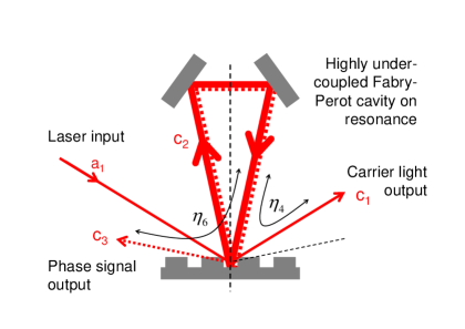
Fig. 2: Three-port-coupled grating in a ring Fabry-Perot interferometer. The grating can be designed such that the laser input is completely sent into port $c_{1}$ on cavity resonance. If the cavity is impedance matched this device might serve as an all-reflective mode-cleaner. Another interesting case occurs in which the cavity is highly under-coupled. Then almost the complete cavity strain signals are sent to port $c_{3}$. Such a device separates carrier light from its modulation sidebands.

From Eq. (14) it can be shown that for a grating with $\eta_{5}^{2}$ at its maximum value for given $\eta_{4}^{2}$ and $\eta_{6}^{2}$, and a cavity on resonance ($\theta=0$) no carrier light from the laser incidenting from the left is leaving the cavity to the left ($c_{3}=0$). This dark port is indicated in Fig. 2 by an arrowed dashed line. If the cavity moves away from resonance for example caused by a cavity strain, amplitude $c_{3}$ is no longer zero. This field is generally termed a phase signal and might appear at some sideband frequency $\Omega$ if the cavity is locked to the time averaged carrier frequency $\omega_{0}$ with locking bandwidth smaller than $\Omega$. The phase signal generated inside the cavity obviously leaves the cavity according to the magnitudes of $\eta_{4}^{2}$ and $\eta_{6}^{2}$ in two directions. From Eqs. (14) and (16) it is easy to prove that the power of the signal indeed splits according to the ratio $\eta_{4}^{2}/\eta_{6}^{2}$. We now discuss two distinct examples; in both of them we consider $\eta_{5}^{2}$ to be designed close to its maximum value. For $\eta_{4}^{2}=\eta_{6}^{2}$ the cavity output coupling is twice the input coupling and the signal is split into two equal halves. We term this case a symmetric or an impedance matched three-port coupled cavity; this is in analogy to the loss-less impedance matched linear cavity whose output coupling is also twice the input coupling. However, due to the choice of $\eta_{5}^{2}$ all the carrier power is sent into port $c_{1}$ if the cavity is on resonance as discussed above. Such a device can serve as an all-reflective mode-cleaner. For $\eta_{4}\!>\!\eta_{6}$ the 3p coupled loss-less cavity can be termed over-coupled and for $\eta_{4}\!<\!\eta_{6}$ under-coupled. As the second example we consider the highly under-coupled grating cavity ($\eta_{4}^{2}\ll\eta_{6}^{2}\ll\eta_{2}^{2}$) and explicitly choose the following coupling coefficients

$$\begin{array}[]{rlrlrl}\!\!\eta_{4}^{2}\!\!\!&=0.0001\,,&\,\eta_{6}^{2}\!\!\!&=0.0099\,,&\,\eta_{2}^{2}\!\!\!&=0.99\,,\\[0.85358pt] \!\!\eta_{5}^{2}\!\!\!&=0.0394\,,&\,\eta_{1}^{2}\!\!\!&=0.9605\,,&\,\eta_{3}^{2}\!\!\!&=0.9507\,,\\ \!\!\phi_{1}\!\!\!&=0\,,&\,\phi_{2}\!\!\!&=0\,,&\,\phi_{3}\!\!\!&=0\,,\\ \!\!\phi_{4}\!\!\!&\approx-3.1349\,,&\,\phi_{5}\!\!\!&\approx 1.5708\,,&\,\phi_{6}\!\!\!&\approx 1.5707\,.\end{array}$$ (17)

For this set of measures again $\eta_{5}^{2}$ is almost at its maximum value and consequently $\eta_{1}^{2}$ and $\eta_{3}^{2}$ are close to their minimum values. As in the impedance matched case described above again all the carrier power is sent into port $c_{1}$. Due to the high asymmetry of the ratio between $\eta_{4}^{2}$ and $\eta_{6}^{2}$ the signal is mainly sent into port $c_{3}$. The special property of the highly under-coupled grating Fabry-Perot interferometer is therefore the possibility of separating carrier light and phase signal. This is a remarkable result. Separation of carrier light and phase signal is well known for a Michelson interferometer operating on a dark fringe. Such an interferometer sends all the laser power back to the laser source. The antisymmetric mode of phase shifts in the Michelson arms is sent into the dark port. The symmetric mode is combined with the reflected laser power and sent towards the bright port. In case of the highly under-coupled 3p grating Fabry-Perot interferometer the almost complete phase signal is separated from carrier light and is accessible to detection and the reflected field in the bright port contains only a marginal fraction of the signal ($\eta_{4}^{2}/\eta_{6}^{2}$).

We point out that all results obtained for the Fabry-Perot ring interferometer using the 3p coupler in Fig. 1b also hold for a linear cavity using the 3p coupler in Fig. 1a. However, some distinctive properties should be mentioned. Regardless of their different topologies the ring FP-interferometer is content with only low efficiencies for greater than zero diffraction orders. All coupling amplitudes in Eqs. (17) with values close to unity describe specular reflections. The production of such a grating with low overall loss should be possible with standard technologies building on the concept used in Refs.[1, 4]. In case of the (highly under-coupled) linear FP-interferometer $\eta_{1}^{2}$ and $\eta_{3}^{2}$ do not describe specular reflections and high diffraction efficiencies in the second order diffraction is required. However, especially in the second order Littrow configuration carrier and signal separation offers the extension by interferometer recycling techniques [5]. Recycling techniques in combination with a grating coupled Fabry-Perot cavity will be subject to an upcoming publication [6].

This work was supported by the Deutsche Forschungsgemeinschaft within the Sonderforschungsbereich TR7. R. Schnabel’s email address is roman.schnabel@aei.mpg.de.

References

[1]A. Bunkowski, O. Burmeister, P. Beyersdorf, K. Danzmann, R. Schnabel, T. Clausnitzer, E.-B. Kley, and A. Tünnermann, Opt. Lett. 29, 2342 (2004).
[2] A. Bunkowski, O. Burmeister, K. Danzmann, and R. Schnabel,
Opt. Lett. 30, 1183 (2005).
[3] A. E. Siegmann, Lasers (University Science Books, Sausalito, California, 1986), pp. 401–408.
[4]T. Clausnitzer, E.-B. Kley, A. Tünnermann, A. Bunkowski, O. Burmeister, K. Danzmann, R. Schnabel, A. Duparré, and S. Gliech,
Opt. Exp. 13, 4370 (2005),
[5]G. Heinzel, K. A Strain, J. Mizuno, K. D. Skeldon, B. Willke, W. Winkler, R. Schilling, A. Rüdiger, and K. Danzmann, Phys. Rev. Lett. 81, 5493 (1998).
[6]A. Bunkowski, O. Burmeister, K. Danzmann, and R. Schnabel, in preparation.