25th June, 2007 Summary
This is an exposé on the use of O’Sullivan penalised splines in contemporary semiparametric regression, including mixed model and Bayesian formulations. O’Sullivan penalised splines are similar to P-splines, but have an advantage of being a direct generalisation of smoothing splines. Exact expressions for the O’Sullivan penalty matrix are obtained. Comparisons between the two reveals that O’Sullivan penalised splines more closely mimic the natural boundary behaviour of smoothing splines. Implementation in modern computing environments such as Matlab, R and BUGS is discussed. Keywords: Additive models, Markov chain Monte Carlo; Mixed models; P-splines; Smoothing splines.

1 Introduction

Splines continue to play a central role in nonparametric and semiparametric regression modelling. Recent synopses include Eubank (1999), Gu (2002), Ruppert, Wand & Carroll (2003) and Denison, Holmes, Mallick & Smith (2002). In all but the last reference, smooth functional relationships are fitted using a large basis of spline functions subject to penalisation. Up until the mid-1990s most literature on spline-based nonparametric regression was concerned with smoothing splines, and their multivariate extension thin plate splines, where the penalty takes a particular form and the number of basis functions roughly equals the sample size (e.g. Wahba, 1990; Green & Silverman, 1994). However, in recent years, there has been a great deal of research on more general spline/penalty strategies, most of which use considerably fewer basis functions. Driving forces include:

• more complicated models, often with several smooth functions;

• larger data sets, where smoothing and thin plate splines become computationally intractable,

• mixed model and Bayesian representations of smoothers that lend themselves to the use of established software, such as BUGS, lme() in R and PROC MIXED in SAS; provided the number of basis functions is relatively low.

Ruppert, Wand & Carroll (2003) summarise and provide access to many of these developments. The term penalised splines has emerged as a descriptor for general spline fitting subject to penalties. O’Sullivan (1986, Section 3) introduced a class of penalised splines based on B-spline basis functions. O’Sullivan penalised splines are a direct generalisation of smoothing splines in that the latter arises when the maximal number of B-spline basis functions are included. Like smoothing splines, O’Sullivan penalised splines possess the attractive feature of natural boundary conditions (e.g. Green & Silverman, 1994, p.12). They have also become the most widely used class of penalised splines in statistical analyses due to their implementation in the popular R and S-PLUS function smooth.spline() and associated generalised additive model software (e.g. the gam library in R; Hastie, 2006). Despite the omnipresence of O’Sullivan penalised splines, their use in semiparametric regression contexts, particularly those involving mixed model and Bayesian representations, is not very common. Recently, Welham, Cullis, Kenward & Thompson (2007) showed how most of the commonly used penalised splines can be treated within a single mixed model framework, although they did not work explicitly with the form given in O’Sullivan (1986). Our contributions in this paper are (a) providing an exact matrix expression for the penalty of O’Sullivan splines that allows implementation in a few lines of a matrix-based computing language, (b) comparison with their closest penalised spline relative, P-splines (Eilers & Marx, 1996), which reveal some noticeable differences near the boundaries, (c) demonstrate explicitly, including with R code, how O’Sullivan splines can be simply added to the mixed model-based regression armoury, and (d) investigate their efficacy in Bayesian semiparametric regression using MCMC software such as BUGS and its variants. We conclude that the several attractive features of O’Sullivan penalised splines — smoothness, numerical stability, natural boundary properties, direct generalisation of smoothing splines — makes them a very good choice of basis in semiparametric regression. Section 2 provides a brief description of O’Sullivan penalised splines. Comparison with P-splines is made in Section 3. Section 4 describes mixed model representation of O’Sullivan penalised splines and how they can be used in models that benefit from this representation. Issues concerning Bayesian penalised spline smoothing and Markov chain Monte Carlo are described in Section 5. O’Sullivan splines of general degree are described in Section 6. Closing discussion is given in Section 7. An appendix contains relevant R code.

2 O’Sullivan Penalised Splines

O’Sullivan penalised splines have already been described several times in the literature. A recent reference is the Chapter 5 Appendix of Hastie, Tibshirani & Friedman (2001). A brief sketch is given here for convenience. Consider the simplest nonparametric regression setting

$$y_{i}=f(x_{i})+\varepsilon_{i},\quad 1\leq i\leq n,$$ (1)

where $(x_{i},y_{i})\in{\mathbb{R}}\times{\mathbb{R}}$. Suppose that an estimate of $f$ is required over $[a,b]$, an interval containing the $x_{i}$’s. For an integer $K\leq n$ let $\kappa_{1},\ldots,\kappa_{K+8}$ be a knot sequence such that

$$a=\kappa_{1}=\kappa_{2}=\kappa_{3}=\kappa_{4}<\kappa_{5}<\cdots<\kappa_{K+4}<\kappa_{K+5}=\kappa_{K+6}=\kappa_{K+7}=\kappa_{K+8}=b$$

and let $B_{1},\ldots,B_{K+4}$ be the cubic B-spline basis functions defined by these knots (see e.g. pp.160–161 of Hastie et al., 2001). Set up the $n\times(K+4)$ design matrix ${\bf B}$ with $(i,k)$ entry $B_{ik}=B_{k}(x_{i})$ and the $(K+4)\times(K+4)$ penalty matrix $\Omega$$\Omega$$\Omega$ with $(k,k^{\prime})$ entry

$${\hbox{\hbox to0.0pt{$\Omega$\hss}\kern 0.25pt\hbox to0.0pt{$\Omega$\hss}\kern 0.25pt$\Omega$}}_{kk^{\prime}}=\int_{a}^{b}B^{\prime\prime}_{k}(x)B_{k^{\prime}}^{\prime\prime}(x)\,dx.$$

Then an estimate of $f$ at location $x\in{\mathbb{R}}$ can be obtained as

$${\widehat{f}}_{\scriptscriptstyle O}(x;\lambda)\equiv{\bf B}_{x}{\widehat{\hbox{\hbox to0.0pt{$\nu$\hss}\kern 0.25pt\hbox to0.0pt{$\nu$\hss}\kern 0.25pt$\nu$}}}_{\scriptscriptstyle O}\quad\mbox{where}\quad{\widehat{\hbox{\hbox to0.0pt{$\nu$\hss}\kern 0.25pt\hbox to0.0pt{$\nu$\hss}\kern 0.25pt$\nu$}}}_{\scriptscriptstyle O}\equiv({\bf B}^{T}{\bf B}+\lambda{\hbox{\hbox to0.0pt{$\Omega$\hss}\kern 0.25pt\hbox to0.0pt{$\Omega$\hss}\kern 0.25pt$\Omega$}})^{-1}{\bf B}^{T}{\bf y},$$ (2)

${\bf B}_{x}\equiv[B_{1}(x),\ldots,B_{K+4}(x)]$ and $\lambda>0$ is a smoothing parameter. Note that the cubic smoothing spline arises in the special case $K=n$ and $\kappa_{k+4}=x_{k}$, $1\leq k\leq n$, provided the $x_{i}$’s are distinct (e.g. Green & Silverman, 1994, Section 3.6). Apart from giving a smooth (twice continuously differentiable) scatterplot smooth, ${\widehat{f}}_{\scriptscriptstyle O}(\cdot;\lambda)$ has good numerical properties. The basis functions are bounded and so not prone to overflow problems. Moreover, ${\bf B}^{T}{\bf B}$ is 4-banded, which leads to $O(n)$ algorithms when $K$ is close to $n$ (e.g. Hastie, et al., 2001). In addition, ${\widehat{f}}_{\scriptscriptstyle O}(\cdot;\lambda)$ satisfies so-called natural boundary conditions, meaning that

$${\widehat{f}}_{\scriptscriptstyle O}^{\prime\prime}(a;\lambda)={\widehat{f}}_{\scriptscriptstyle O}^{\prime\prime\prime}(a;\lambda)={\widehat{f}}_{\scriptscriptstyle O}^{\prime\prime}(b;\lambda)={\widehat{f}}_{\scriptscriptstyle O}^{\prime\prime\prime}(b;\lambda)=0$$

and implying that ${\widehat{f}}_{\scriptscriptstyle O}(\cdot;\lambda)$ is linear over $[a,\kappa_{5}]$ and $[\kappa_{K+4},b]$. Figure 1 illustrates these natural boundary properties of ${\widehat{f}}_{\scriptscriptstyle O}(\cdot;\lambda)$ for data on ratios of strontium isotopes found in fossil shells and their age; see Chaudhuri & Marron (1999) for details. Also, ${\widehat{f}}_{\scriptscriptstyle O}(\cdot;\lambda)$ approximates the least squares line as $\lambda\to\infty$. The implication for mixed model smoothing is that the induced fixed effects component corresponds to straight line basis functions. Details are given in Section 4.

Figure 1: Illustration of natural boundary properties of a 20-interior knot O’Sullivan penalised spline fit to the fossil data over the interval $[85,130]$ millions of years. The interior knots are shown as solid diamonds ($\blacklozenge$). Inset: The 24 B-spline basis functions.

Computation of the design matrix ${\bf B}$ is usually quite easy. For example, B-splines are readily available in the Matlab, R and S-PLUS computing environments. Otherwise recurrence formulae (e.g. de Boor, 1978; Eilers & Marx, 1996) can be called upon. However, computation of $\Omega$$\Omega$$\Omega$ requires some additional effort. In Section 6, while treating general degree O’Sullivan penalised splines, we derive an exact matrix algebraic expression for the corresponding penalty matrices. In the cubic case our theorem reduces to the expression:

$${\hbox{\hbox to0.0pt{$\Omega$\hss}\kern 0.25pt\hbox to0.0pt{$\Omega$\hss}\kern 0.25pt$\Omega$}}=({\widetilde{\bf B}}^{\prime\prime})^{T}\mbox{\rm diag}({\bf w}){\widetilde{\bf B}}^{\prime\prime}$$ (3)

where ${\widetilde{\bf B}}^{\prime\prime}$ is the $3(K+7)\times(K+4)$ matrix with $(i,j)$ entry $B^{\prime\prime}_{j}({\widetilde{x}}_{i})$, ${\widetilde{x}}_{i}$ is the $i$th entry of the vector

$${\widetilde{\bf x}}=\left(\kappa_{1},\frac{\kappa_{1}+\kappa_{2}}{2},\kappa_{2},\kappa_{2},\frac{\kappa_{2}+\kappa_{3}}{2},\kappa_{3},\ldots,\kappa_{K+7},\frac{\kappa_{K+7}+\kappa_{K+8}}{2},\kappa_{K+8}\right).$$

and ${\bf w}$ is the $3(K+7)\times 1$ vector given by

$${\bf w}=\left(\textstyle{\frac{1}{6}}(\Delta{\hbox{\hbox to0.0pt{$\kappa$\hss}\kern 0.25pt\hbox to0.0pt{$\kappa$\hss}\kern 0.25pt$\kappa$}})_{1},\textstyle{\frac{4}{6}}(\Delta{\hbox{\hbox to0.0pt{$\kappa$\hss}\kern 0.25pt\hbox to0.0pt{$\kappa$\hss}\kern 0.25pt$\kappa$}})_{1},\textstyle{\frac{1}{6}}(\Delta{\hbox{\hbox to0.0pt{$\kappa$\hss}\kern 0.25pt\hbox to0.0pt{$\kappa$\hss}\kern 0.25pt$\kappa$}})_{1},\textstyle{\frac{1}{6}}(\Delta{\hbox{\hbox to0.0pt{$\kappa$\hss}\kern 0.25pt\hbox to0.0pt{$\kappa$\hss}\kern 0.25pt$\kappa$}})_{2},\textstyle{\frac{4}{6}}(\Delta{\hbox{\hbox to0.0pt{$\kappa$\hss}\kern 0.25pt\hbox to0.0pt{$\kappa$\hss}\kern 0.25pt$\kappa$}})_{2},\textstyle{\frac{1}{6}}(\Delta{\hbox{\hbox to0.0pt{$\kappa$\hss}\kern 0.25pt\hbox to0.0pt{$\kappa$\hss}\kern 0.25pt$\kappa$}})_{2},\ldots,\textstyle{\frac{1}{6}}(\Delta{\hbox{\hbox to0.0pt{$\kappa$\hss}\kern 0.25pt\hbox to0.0pt{$\kappa$\hss}\kern 0.25pt$\kappa$}})_{K+7},\textstyle{\frac{4}{6}}(\Delta{\hbox{\hbox to0.0pt{$\kappa$\hss}\kern 0.25pt\hbox to0.0pt{$\kappa$\hss}\kern 0.25pt$\kappa$}})_{K+7},\textstyle{\frac{1}{6}}(\Delta{\hbox{\hbox to0.0pt{$\kappa$\hss}\kern 0.25pt\hbox to0.0pt{$\kappa$\hss}\kern 0.25pt$\kappa$}})_{K+7}\right),$$

where $(\Delta{\hbox{\hbox to0.0pt{$\kappa$\hss}\kern 0.25pt\hbox to0.0pt{$\kappa$\hss}\kern 0.25pt$\kappa$}})_{k}\equiv\kappa_{k+1}-\kappa_{k}$, $1\leq k\leq K+7$. Result (3) is none other than Simpson’s rule applied over each of the inter-knot differences. This is because each $B_{i}^{\prime\prime}B_{j}^{\prime\prime}$ function is piecewise quadratic. For commonly used values of $K$, (3) allows straightforward computation of $\Omega$$\Omega$$\Omega$ in matrix-based languages such as Matlab, R and S-PLUS. In the Appendix we demonstrate computation of $\Omega$$\Omega$$\Omega$ in 4 lines of R code. Lastly, we mention knot choice. The R and S-PLUS function smooth.spline() uses

$$\kappa_{k}\simeq\left({k+1}\over K+2\right)\mbox{th sample quantile of the $x_{i}$'s}$$

where

$$K=\left\{\begin{array}[]{ll}n&n<50\\ 100&n=200\\ 140&n=800\\ 200+(n-3200)^{1/5}&n>3200.\\ \end{array}\right.$$

Other values of $n$ between 50 and 3200 are handled via a logarithmic interpolation. For many functional relationships, fewer knots are sufficient. Figure 1 is one example, where only $K=20$ interior knots are used without compromising the quality of the fit. A common default in the penalised spline literature is $K=\min(n_{U}/4,35)$, where $n_{U}$ is the number of unique $x_{i}$’s (e.g. Ruppert et al., 2003). Ruppert (2002) discusses ‘hi-tech’ choice of $K$. The distribution of the knots, for a given $K$, may have some affect on the results. As mentioned above, smooth.spline() uses quantile-based knots while e.g. Eilers & Marx (1996) recommend equally-spaced knots. In most situations this effect will be minor. However, for either strategy, it is possible to construct regression functions and predictor variable distributions for which problems arise. More sophisticated knot placement strategies may help. For example, Luo & Wahba (1997) propose more sophisticated basis function reduction methods that could be adapted to the current context.

3 Comparison with P-splines

The closest relatives of O’Sullivan penalised splines are the P-splines of Eilers & Marx (1996). If the interior knots $\kappa_{5},\ldots,\kappa_{K+4}$ are taken to be equally-spaced then the family of cubic P-splines is given by (2) with the $\Omega$$\Omega$$\Omega$ replaced by ${\bf D}_{k}^{T}{\bf D}_{k}$, where ${\bf D}_{k}$ is the $k$th-order differencing matrix. This differencing penalty corresponds to a discrete approximation to the integrated square of the $k$th derivative of the B-spline smoother. The choice $k=2$ leads to the cubic P-spline estimate

$${\widehat{f}}_{\scriptscriptstyle P}(x;\lambda)={\bf B}_{x}{\widehat{\hbox{\hbox to0.0pt{$\nu$\hss}\kern 0.25pt\hbox to0.0pt{$\nu$\hss}\kern 0.25pt$\nu$}}}_{\scriptscriptstyle P},\quad\mbox{where}\quad{\widehat{\hbox{\hbox to0.0pt{$\nu$\hss}\kern 0.25pt\hbox to0.0pt{$\nu$\hss}\kern 0.25pt$\nu$}}}_{\scriptscriptstyle P}\equiv({\bf B}^{T}{\bf B}+\lambda{\bf D}_{2}^{T}{\bf D}_{2})^{-1}{\bf B}^{T}{\bf y},$$ (4)

having the property that ${\widehat{f}}_{\scriptscriptstyle P}(\cdot;\lambda)$ approaches the least squares line as $\lambda\to\infty$. In this sense, (4) is the closest relative of ${\widehat{f}}_{\scriptscriptstyle O}(\cdot;\lambda)$. If the interior knots are equally-spaced then the bands in the interior rows are, up to multiplicative factors, as follows:

$$\begin{array}[]{lrrrrrrr}\mbox{O'Sullivan penalised splines (\ref{eq:fhat.osu}):}&\ \ \ \ 5,&0,&-45,&80,&-45,&0,&5\\ \mbox{Cubic P-splines; 2nd order diff. (\ref{eq:fhat.psp}):}&\ \ \ \ -4,&24,&-60,&80,&-60,&24,&-4\\ \end{array}$$

Figure 2 facilitates visual comparison of the two. It is seen that the differences are relatively small, although not negligible.

Figure 2: Comparison of near-diagonal entries of the penalty matrices for O’Sullivan penalised splines and cubic P-splines with $k=2$ and equally-spaced interior knots.

What are the relative advantages of smoothers based on cubic P-splines and O’Sullivan penalised splines, or O-splines for short? Theoretical comparison between P-splines and O-splines in terms of estimation performance, perhaps in the spirit of Hall & Opsomer (2005), would be ideal – although beyond the scope of the current paper. Eilers and Marx (1996) partially justify use of P-splines rather than O’Sullivan splines based on simplicity of the P-spline penalty matrix. However, as seen from (3), the penalty matrix needed for O-splines can be obtained straightforwardly. Furthermore the discrete approximation of P-splines requires equally-spaced knots which, depending on $f$, may not be desirable, A possible advantage of P-splines is the option of higher-order penalties, although the resulting smoothers can have erratic extrapolation behaviour. A possible advantage of O-splines is their direct relationship with time-honoured smoothing splines, and their attractive theoretical properties (e.g. Nussbaum, 1985). ¿From the results described in Section 2 is clear that O-splines approach smoothing splines as $K\to n$. But how close are O-splines to smoothing splines for common (smaller) choices of $K$, and are they closer than P-splines with the same value of $K$ and interior knots? To address these questions we conducted an empirical study based on the eighteen homoscedastic nonparametric regression settings in Wand (2000). For O-splines we used $K=100$ equally spaced interior knots with 4 repeated knots at each boundary as described in Section 2. However, for P-splines we used the knot sequence described in the Appendix of Eilers & Marx (1996) which involves extending the knots beyond the boundary rather than repeating them. For each setting 200 samples were generated and smoothing spline estimates ${\widehat{f}}_{\scriptscriptstyle S}$, with smoothing parameter chosen via generalised cross-validation, were obtained. We then computed ${\widehat{f}}_{\scriptscriptstyle O}$ and ${\widehat{f}}_{\scriptscriptstyle P}$ to have the same effective degrees of freedom as ${\widehat{f}}_{\scriptscriptstyle S}$ and recorded closeness measures $d({\widehat{f}}_{\scriptscriptstyle O},{\widehat{f}}_{\scriptscriptstyle S};A)$ and $d({\widehat{f}}_{\scriptscriptstyle P},{\widehat{f}}_{\scriptscriptstyle S};A)$ where

$$d(f,g;A)\equiv\int_{A}(f-g)^{2}.$$

We took $A$ corresponding to the intervals $(a,\kappa_{5})$ (left boundary), $(\kappa_{5},\kappa_{K+5})$ (interior), $(\kappa_{K+5},b)$ (right boundary) and $(a,b)$ (total region) where the $\kappa_{k}$ denote the knots used for the O-spline fits. The Wand (2000) settings all involve predictor data within the unit interval. We took $(a,b)=(-0.1,1.1)$ to assess behaviour beyond the range of the data. Wilcoxon tests on the 200 differences $d({\widehat{f}}_{\scriptscriptstyle O},{\widehat{f}}_{\scriptscriptstyle S};A)-d({\widehat{f}}_{\scriptscriptstyle P},{\widehat{f}}_{\scriptscriptstyle S};A)$ were carried out for each setting and choice of $A$. Apart from being distribution-free, Wilcoxon tests have the advantage of being invariant to normalisation and whether differences or ratios are used. In all 72 cases O-splines were closer to smoothing splines than P-splines in the sense that the Wilcoxon p-value$<0.01$. To appreciate the practical significance of these results we plotted the data and estimates at the 90th percentiles of each of the $d({\widehat{f}}_{\scriptscriptstyle O},{\widehat{f}}_{\scriptscriptstyle S};A)$ and $d({\widehat{f}}_{\scriptscriptstyle P},{\widehat{f}}_{\scriptscriptstyle S};A)$ samples, corresponding to relatively high discrepancies. Some examples are shown in Figure 3.

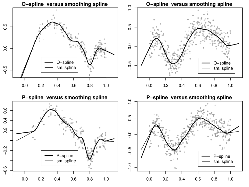
Figure 3: O-spline and P-spline fits compared with smoothing spline fits corresponding to the 90th percentiles of the $d({\widehat{f}}_{\scriptscriptstyle O},{\widehat{f}}_{\scriptscriptstyle S};A)$ and $d({\widehat{f}}_{\scriptscriptstyle P},{\widehat{f}}_{\scriptscriptstyle S};A)$ samples; for two of the homoscedastic settings of Wand (2000).

In the interior all estimates of the same data, and same degrees of freedom, are almost indistinguishable with the naked eye. However, big differences occur at the boundary. P-splines have a tendency to deviate from the natural boundary behaviour of smoothing splines. We also observed this phenomenom in the other 16 settings. Further study into this differing extrapolation behaviour would be worthwhile. We speculate that it comes from differences between the exact integral penalty and its discrete approximation near the boundary.

4 Mixed Model Formulation

There are several ways by which ${\widehat{\hbox{\hbox to0.0pt{$\nu$\hss}\kern 0.25pt\hbox to0.0pt{$\nu$\hss}\kern 0.25pt$\nu$}}}_{\scriptscriptstyle O}$ in (2) can be expressed as a best linear unbiased predictor (BLUP) in a mixed model (e.g. Speed, 1990; Verbyla, 1994). However, from a software standpoint, the most convenient form is ${\widehat{\hbox{\hbox to0.0pt{$\nu$\hss}\kern 0.25pt\hbox to0.0pt{$\nu$\hss}\kern 0.25pt$\nu$}}}_{\scriptscriptstyle O}=({\widehat{\hbox{\hbox to0.0pt{$\beta$\hss}\kern 0.25pt\hbox to0.0pt{$\beta$\hss}\kern 0.25pt$\beta$}}},{\widehat{\bf u}})$ where ${\widehat{\hbox{\hbox to0.0pt{$\beta$\hss}\kern 0.25pt\hbox to0.0pt{$\beta$\hss}\kern 0.25pt$\beta$}}}$ and ${\widehat{\bf u}}$ are (empirical) BLUPs of $\beta$$\beta$$\beta$ and ${\bf u}$ in the mixed model

$${\bf y}={\bf X}{\hbox{\hbox to0.0pt{$\beta$\hss}\kern 0.25pt\hbox to0.0pt{$\beta$\hss}\kern 0.25pt$\beta$}}+{\bf Z}{\bf u}+{\hbox{\hbox to0.0pt{$\varepsilon$\hss}\kern 0.25pt\hbox to0.0pt{$\varepsilon$\hss}\kern 0.25pt$\varepsilon$}},\quad\left[\begin{array}[]{c}{\bf u}\\ {\hbox{\hbox to0.0pt{$\varepsilon$\hss}\kern 0.25pt\hbox to0.0pt{$\varepsilon$\hss}\kern 0.25pt$\varepsilon$}}\\ \end{array}\right]\sim N\left(\left[\begin{array}[]{c}{\bf 0}\\ {\bf 0}\\ \end{array}\right],\left[\begin{array}[]{cc}\sigma_{u}^{2}{\bf I}&{\bf 0}\\ {\bf 0}&\sigma_{\varepsilon}^{2}{\bf I}\\ \end{array}\right]\right)$$ (5)

for some design matrices ${\bf X}$ and ${\bf Z}$. An explicit expression for the BLUP in (5) (e.g. Ruppert, Wand & Carroll, 2003; Section 4.5.3) is

$$\left[\begin{array}[]{c}{\widehat{\hbox{\hbox to0.0pt{$\beta$\hss}\kern 0.25pt\hbox to0.0pt{$\beta$\hss}\kern 0.25pt$\beta$}}}\\ {\widehat{\bf u}}\\ \end{array}\right]={\widehat{\hbox{\hbox to0.0pt{$\nu$\hss}\kern 0.25pt\hbox to0.0pt{$\nu$\hss}\kern 0.25pt$\nu$}}}_{\scriptscriptstyle O}=\left({\bf C}^{T}{\bf C}+\lambda\left[\begin{array}[]{cc}{\bf 0}&\ \ \ {\bf 0}\\ {\bf 0}&\ \ \ {\bf I}\\ \end{array}\right]\right)^{-1}{\bf C}^{T}{\bf y},\quad\lambda=\sigma_{u}^{2}/\sigma^{2}_{\varepsilon},$$

where ${\bf C}=[{\bf X}|{\bf Z}]$, ${\bf I}$ is the identity matrix with the same number of columns as ${\bf Z}$. This ‘canonical form’ can be achieved if a $(K+4)\times(K+4)$ linear transformation matrix ${\bf L}$ can be found such that ${\bf C}={\bf B}{\bf L}$ and

$${\bf L}^{T}{\hbox{\hbox to0.0pt{$\Omega$\hss}\kern 0.25pt\hbox to0.0pt{$\Omega$\hss}\kern 0.25pt$\Omega$}}{\bf L}=\left[\begin{array}[]{cc}{\bf 0}&\ \ \ {\bf 0}\\ {\bf 0}&\ \ \ {\bf I}\\ \end{array}\right].$$

The usual method for obtaining ${\bf L}$ is spectral decomposition (e.g. Nychka & Cummins, 1996; Cantoni & Hastie, 2002; Welham et al., 2007). It follows from results in the smoothing spline literature (e.g. Speed, 1991, Section 6) that

$$\mbox{rank}({\hbox{\hbox to0.0pt{$\Omega$\hss}\kern 0.25pt\hbox to0.0pt{$\Omega$\hss}\kern 0.25pt$\Omega$}})=K+2.$$

Hence, the spectral decomposition of $\Omega$$\Omega$$\Omega$ is of the form ${\hbox{\hbox to0.0pt{$\Omega$\hss}\kern 0.25pt\hbox to0.0pt{$\Omega$\hss}\kern 0.25pt$\Omega$}}={\bf U}\mbox{diag}({\bf d}){\bf U}^{T}$ where ${\bf U}^{T}{\bf U}={\bf I}$ and ${\bf d}$ is a $(K+4)\times 1$ vector with exactly 2 zero entries and $K+2$ positive entries. Let ${\bf d}_{\scriptscriptstyle Z}$ be the $(K+2)\times 1$ sub-vector of ${\bf d}$ containing these positive entries, and let ${\bf U}_{\scriptscriptstyle Z}$ be the $(K+4)\times(K+2)$ sub-matrix of ${\bf U}$ with columns corresponding to positive entries of ${\bf d}$. Then an appropriate linear transformation is ${\bf L}=[{\bf U}_{\scriptscriptstyle X}|{\bf U}_{\scriptscriptstyle Z}\mbox{diag}({\bf d}_{\scriptscriptstyle Z}^{-1/2})]$. This leads to the fixed and random effects design matrices:

$${\bf X}={\bf B}{\bf U}_{\scriptscriptstyle X}\quad\mbox{and}\quad{\bf Z}={\bf B}{\bf U}_{\scriptscriptstyle Z}\mbox{diag}({\bf d}_{\scriptscriptstyle Z}^{-1/2}).$$ (6)

However, following again from the aforementioned smoothing spline literature (e.g. Speed, 1991, Section 6), ${\bf B}{\bf U}_{\scriptscriptstyle X}$ is a basis for the space of straight lines so the simpler specification ${\bf X}=[1\ x_{i}]_{1\leq i\leq n}$ may be used instead without affecting the fit. The spline basis formed through spectral decomposition of more familiar bases is known as the Demmler-Reinsch basis (e.g. Nychka & Cummins, 1996). Figure 4 allows comparison of the original B-spline basis, corresponding to ${\bf B}$, and the Demmler-Reinsch basis corresponding to ${\bf Z}$. Notice the damping of the ${\bf Z}$ basis functions with increasing oscillation. This compensates for the fact that the penalty is a multiple of the identity matrix.

Figure 4: Comparison of B-spline basis and Demmler-Reinsch basis for the fossil data example of Figure 2. The interior knots are shown as solid diamonds ($\blacklozenge$).

In the Appendix it is shown how the R linear mixed model function lme() can be used to obtain ${\widehat{f}}_{\scriptscriptstyle O}(\cdot;\lambda)$ based on (5), with ${\bf Z}$ given by (6). For simple scatterplot smoothing there is little difference between this approach and direct use of smooth.spline(), and the answers are equivalent if the knot sequence and $\lambda$ values are equal. The default choice of $\lambda$ differs: lme() uses restricted maximum likelihood (REML) to choose $\lambda$, while smooth.spline() uses generalised cross-validation (GCV). The main advantage of the mixed model formulation of penalised splines is the incorporation into more complex models. Several examples are given in, for example, Ruppert, Wand & Carroll (2003). We will briefly describe one of them here. Figure 5 displays a longitudinal data set on bone mineral acquisition in young females (source: Bachrach, Hastie, Wang, Narasimhan & Marcus, 1999). The data consists of spinal bone mineral density (SBMD) measurements on each of 230 female subjects aged between 8 and 27. Each subject is measured between one and four times. Let $n_{i}$ denote the number of measurements for subject $i$. The subjects have been divided into four ethnic groups: Asian, Black, Hispanic and White.

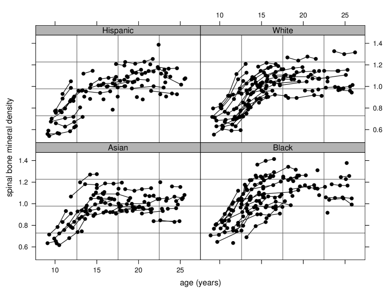
Figure 5: The spinal bone mineral data. Lines connect measurements taken on the same subject.

A useful additive mixed model for these data is:

$${\tt SBMD}_{ij}=U_{i}+f({\tt age}_{ij})+\beta_{1}{\tt Black_{i}}+\beta_{2}{\tt Hispanic_{i}}+\beta_{3}{\tt White_{i}}+\varepsilon_{ij},\quad 1\leq i\leq 230,\quad 1\leq j\leq n_{i}\quad$$ (7)

where $U_{i}\ \mbox{i.i.d.}\ N(0,\sigma_{u}^{2})$ are random intercepts for each subject, and ${\tt Black}_{i}$, ${\tt Hispanic}_{i}$ and ${\tt White}_{i}$ are ethnicity indicators. $\varepsilon_{ij}\ \mbox{i.i.d.}\ N(0,\sigma_{\varepsilon}^{2})$ are random errors. More sophisticated models that account for, say, serial correlation could be entertained. O’Sullivan penalised splines can be used to fit (7) with the design matrices set up as follows. Based on the ${\tt age}_{i}$ values and appropriate knots, set up

$${\bf Z}_{\mbox{{\tiny spline}}}={\bf B}{\bf U}_{\scriptscriptstyle Z}\mbox{diag}({\bf d}_{\scriptscriptstyle Z}^{-1/2})$$

analogous to the ${\bf Z}$ matrix of (6) for simple scatterplot smoothing. In the Appendix, when fitting data of this type, we use 15 interior knots corresponding to quantiles of the unique age values. Form

$${\bf X}=\left[\begin{array}[]{ccccc}1&{\tt age}_{11}&{\tt Black}_{1}&{\tt Hispanic}_{1}&{\tt White}_{1}\\ \vdots&\vdots&\vdots&\vdots&\vdots\\ 1&{\tt age}_{1n_{1}}&{\tt Black}_{1}&{\tt Hispanic}_{1}&{\tt White}_{1}\\ \vdots&\vdots&\vdots&\vdots&\vdots\\ 1&{\tt age}_{230,1}&{\tt Black}_{230}&{\tt Hispanic}_{230}&{\tt White}_{230}\\ \vdots&\vdots&\vdots&\vdots&\vdots\\ 1&{\tt age}_{230,n_{230}}&{\tt Black}_{230}&{\tt Hispanic}_{230}&{\tt White}_{230}\\ \end{array}\right]\ \mbox{and}\ {\bf Z}_{\mbox{{\tiny subj}}}=\left[\begin{array}[]{cccc}1&0&\cdots&0\\ \vdots&\vdots&\cdots&\vdots\\ 1&0&\cdots&0\\ \vdots&\vdots&\ddots&\vdots\\ 0&0&\cdots&1\\ \vdots&\vdots&\cdots&\vdots\\ 0&0&\cdots&1\\ \end{array}\right].$$

Concatenate ${\bf Z}_{\mbox{{\tiny subj}}}$ and ${\bf Z}_{\mbox{{\tiny spline}}}$ to form

$${\bf Z}=[{\bf Z}_{\mbox{{\tiny subj}}}|{\bf Z}_{\mbox{{\tiny spline}}}].$$

The appropriate mixed model is then

$${\bf y}={\bf X}{\hbox{\hbox to0.0pt{$\beta$\hss}\kern 0.25pt\hbox to0.0pt{$\beta$\hss}\kern 0.25pt$\beta$}}+{\bf Z}{\bf u}+\mbox{\boldmath$\varepsilon$},\quad\mbox{Cov}\left[\begin{array}[]{c}{\bf u}\\ \mbox{\boldmath$\varepsilon$}\end{array}\right]=\left[\begin{array}[]{ccc}\sigma_{U}^{2}{\bf I}&{\bf 0}&{\bf 0}\\ {\bf 0}&\sigma_{u}^{2}{\bf I}&{\bf 0}\\ {\bf 0}&{\bf 0}&\sigma^{2}_{\varepsilon}{\bf I}\\ \end{array}\right].$$ (8)

The Appendix contains R code for fitting this model. Note, in particular, that it circumvents explicit specification of ${\bf Z}_{\mbox{{\tiny subj}}}$. This is important for large longitudinal datasets.

5 Bayesian Analysis and Markov Chain Monte Carlo

A particularly attractive advantage of penalised splines, compared with smoothing splines, is the ease with which they can be fed into Markov Chain Monte Carlo (MCMC) schemes for fitting Bayesian semiparametric regression models – due to the reduction in the number of basis functions. For simple scatterplot smoothing this involves the Bayesian version of (5):

$${\bf y}|{\hbox{\hbox to0.0pt{$\beta$\hss}\kern 0.25pt\hbox to0.0pt{$\beta$\hss}\kern 0.25pt$\beta$}},{\bf u},\sigma_{\varepsilon}^{2}\sim N({\bf X}{\hbox{\hbox to0.0pt{$\beta$\hss}\kern 0.25pt\hbox to0.0pt{$\beta$\hss}\kern 0.25pt$\beta$}}+{\bf Z}{\bf u},\sigma_{\varepsilon}^{2}{\bf I}),\quad{\bf u}|\sigma_{u}^{2}\sim N({\bf 0},\sigma_{u}^{2}{\bf I})$$

and suitable (usually diffuse) prior distributions for $\beta$$\beta$$\beta$, $\sigma_{u}^{2}$ and $\sigma_{\varepsilon}^{2}$. However, the big advantages of a Bayesian/MCMC approach are realised when handling complications such as measurement error (e.g. Carroll, Ruppert, Stefanski & Crainiceanu, 2006) and generalised responses (e.g. Zhao, Staudenmayer, Coull & Wand, 2006), which are hindered by intractable integrals in the likelihood. Crainiceanu, Ruppert & Wand (2005) focus on use of the MCMC package WinBUGS (Windows version of BUGS, Spiegelhalter, Thomas & Best, 2000) for Bayesian penalised spline models. They reported that the choice of basis functions can have a substantial impact on the convergence of the chain. We decided to conduct some convergence checks for MCMC fitting of the regression model:

$$\mbox{logit}\{P(\mbox{\tt union}_{i}=1|\mbox{\tt wage}_{i})\}=f(\mbox{\tt wage}_{i})$$ (9)

with $f$ estimated via O’Sullivan penalised splines. Here $({\tt wage}_{i},{\tt union}_{i})$, $1\leq i\leq 534$, are pairs of wage amounts (dollars per hour) and trade union membership indicators for a sample of U.S. workers (source: Berndt, 1991). We expressed (9) as the Bayesian logistic mixed model:

$$\mbox{logit}\{P(\mbox{\tt union}_{i}=1|\mbox{\tt wage}_{i})\}=({\bf X}{\hbox{\hbox to0.0pt{$\beta$\hss}\kern 0.25pt\hbox to0.0pt{$\beta$\hss}\kern 0.25pt$\beta$}}+{\bf Z}{\bf u})_{i},\quad 1\leq i\leq 534$$

where ${\bf X}=[1\ {\tt wage}_{i}]_{1\leq i\leq 534}$ and ${\bf Z}={\bf B}{\bf U}_{\scriptscriptstyle Z}\mbox{diag}({\bf d}_{\scriptscriptstyle Z}^{-1/2})$, using the notation of Section 4. We used 15 interior knots with quantile spacing.

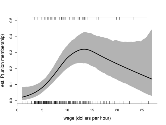
Figure 6: Fit of (9) using O’Sullivan penalised splines.

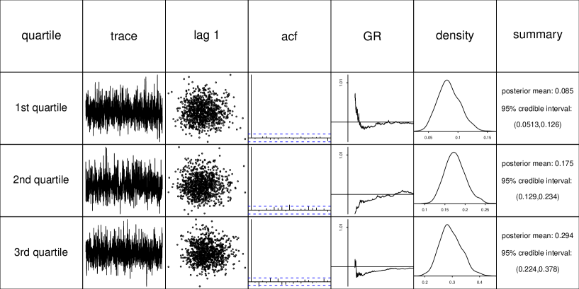
Figure 7: Assessment of MCMC convergence for O’Sullivan penalised spline estimation of (9) at each quartile of wage. The columns are: quartile of wage, trace plot of sample of corresponding coefficient, plot of sample against 1-lagged sample, sample autocorrelation function, Gelman-Rubin $\surd{{\widehat{R}}}$ diagnostic, kernel estimates posterior density and basic numerical summaries.

Following the advice of Zhao et al. (2006) we used WinBUGS to generate chains of length 5000 after a burn-in of 5000 and applied a thinning factor of 5, resulting in posterior samples of size 1000. Also in keeping with the recommendations of Zhao et al. (2006) we placed diffuse priors on the fixed effect parameters and variance component: $\beta_{0},\beta_{1}$ independent $N(0,10^{8})$ and the prior density of $\sigma_{u}^{2}$ proportional to $(\sigma_{u}^{2})^{-1.01}e^{-1/(100\sigma_{u}^{2})}$, the Inverse Gamma distribution with shape and rate parameter both 0.01, after scaling the predictor to have unit variance. Zhao et al. (2006) found that the results can be sensitive to the choice of the Inverse Gamma hyperparameter. The pointwise posterior mean effect of wage on the probability of trade union membership, together with 95% pointwise credible sets, is shown in Figure 6. Figure 7 allows assessment of convergence of the MCMC at each quartile of the wage sample and is seen to be excellent in each case. We also conducted convergence checks for larger logistic additive models involving up to 6 predictors and 3 smooth functions and found the mixing to be very good when O-splines were used. Several examples of semiparametric regression with WinBUGS, including code, are given in Crainiceanu et al.(2005) and Zhao et al.(2006).

6 General Degree Extension

Cubic O’Sullivan penalised splines have a natural extension to general odd degree splines. Higher degree splines have a role to play when smoother curve estimates are required. This arises, for example, in feature significance methodology (e.g. Chaudhuri & Marron, 1999; Hannig & Marron, 2006) where first and second derivatives of the fit are required. Return to the simple nonparametric regression setting (1) and let $m$ be a general positive integer. Form the knot sequence

$$a=\kappa_{1}=\ldots=\kappa_{2m}<\kappa_{2m+1}<\ldots<\kappa_{2m+K}<\kappa_{2m+K+1}=\ldots=\kappa_{4m+K}=b$$

and let $B_{2m-1,1},\ldots,B_{2m-1,K+2m}$ be the degree $(2m-1)$ B-spline basis defined by these knots. Order $m$ O’Sullivan penalised splines then take the general form

$${\widehat{f}}_{\scriptscriptstyle O}(x;m,\lambda)\equiv{\bf B}_{2m-1,x}{\widehat{\hbox{\hbox to0.0pt{$\nu$\hss}\kern 0.25pt\hbox to0.0pt{$\nu$\hss}\kern 0.25pt$\nu$}}}_{\scriptscriptstyle O}\quad\mbox{where}\quad{\widehat{\hbox{\hbox to0.0pt{$\nu$\hss}\kern 0.25pt\hbox to0.0pt{$\nu$\hss}\kern 0.25pt$\nu$}}}_{\scriptscriptstyle O}\equiv({\bf B}_{2m-1}^{T}{\bf B}_{2m-1}+\lambda{\hbox{\hbox to0.0pt{$\Omega$\hss}\kern 0.25pt\hbox to0.0pt{$\Omega$\hss}\kern 0.25pt$\Omega$}}^{(m)})^{-1}{\bf B}_{2m-1}^{T}{\bf y}.$$

Here ${\bf B}_{2m-1}$ is the $n\times(K+4m)$ design matrix with $(i,k)$ entry $B_{{2m-1},k}(x_{i})$, ${\bf B}_{2m-1,x}=[B_{2m-1,1}(x),\ldots,B_{2m-1,K+2m}(x)]$ and ${\hbox{\hbox to0.0pt{$\Omega$\hss}\kern 0.25pt\hbox to0.0pt{$\Omega$\hss}\kern 0.25pt$\Omega$}}^{(m)}$ is the $(K+2m)\times(K+2m)$ penalty matrix with $(k,k^{\prime})$ entry

$${\hbox{\hbox to0.0pt{$\Omega$\hss}\kern 0.25pt\hbox to0.0pt{$\Omega$\hss}\kern 0.25pt$\Omega$}}^{(m)}_{kk^{\prime}}=\int_{a}^{b}B_{2m-1,k}^{(m)}(x)B_{2m-1,k^{\prime}}^{(m)}(x)\,dx.$$

In the special case where the interior knots coincide with the $x_{i}$’s, assumed distinct, ${\widehat{f}}_{\scriptscriptstyle O}(\cdot;m,\lambda)$ corresponds to the order $m$ smoothing spline; i.e. the minimiser of

$$\sum_{i=1}^{n}\{y_{i}-f(x_{i})\}^{2}+\lambda\int_{a}^{b}f^{(m)}(x)^{2}\,dx$$

(e.g. Schoenberg, 1964). We are now ready to state our result for exact computation of O’Sullivan spline penalty matrices: Theorem. The penalty matrix ${\hbox{\hbox to0.0pt{$\Omega$\hss}\kern 0.25pt\hbox to0.0pt{$\Omega$\hss}\kern 0.25pt$\Omega$}}^{(m)}$ admits the exact explicit expression

$${\hbox{\hbox to0.0pt{$\Omega$\hss}\kern 0.25pt\hbox to0.0pt{$\Omega$\hss}\kern 0.25pt$\Omega$}}^{(m)}=({\widetilde{\bf B}}^{(m)})^{T}\mbox{\rm diag}({\bf w}){\widetilde{\bf B}}^{(m)}$$

where ${\widetilde{\bf B}}^{(m)}$ is the $(2m-1)(K+4m-1)\times(K+2m)$ matrix with $(i,j)$ entry $B_{2m-1,j}^{(m)}({\widetilde{x}}_{i})$ and ${\bf w}$ is a $(2m-1)(K+4m-1)\times 1$ vector with $i$th entry $w_{i}$. The ${\widetilde{x}}_{i}$ and $w_{i}$ values are obtained according to

$${\widetilde{x}}_{(2m-1)(\ell-1)+\ell^{\prime}+1}=\kappa_{\ell}+\ell^{\prime}h_{m,\ell},\quad w_{(2m-1)(\ell-1)+\ell^{\prime}+1}=h_{m,\ell}\omega_{m,\ell^{\prime}}$$

for $1\leq\ell\leq K+4m-1$, $0\leq\ell^{\prime}\leq 2m-2$. Here, for $1\leq k\leq K+2m$, $h_{1,k}=\kappa_{k+1}-\kappa_{k}$ and, for $m\geq 2$, $h_{m,k}=(\kappa_{k+1}-\kappa_{k})/(2m-2)$. Lastly, for all $m\geq 1$,

$$\omega_{m,k}=\frac{(-1)^{k}}{k!(2m-2-k)!}\int_{0}^{2m-2}\frac{t(t-1)\cdots(t-2m+2)}{t-k}\,dt,\quad k=0,\ldots,{2m-2}.$$

Proof. The $(k,k^{\prime})$ entry of ${\hbox{\hbox to0.0pt{$\Omega$\hss}\kern 0.25pt\hbox to0.0pt{$\Omega$\hss}\kern 0.25pt$\Omega$}}^{(m)}$ is

$${\hbox{\hbox to0.0pt{$\Omega$\hss}\kern 0.25pt\hbox to0.0pt{$\Omega$\hss}\kern 0.25pt$\Omega$}}^{(m)}_{kk^{\prime}}=\int_{a}^{b}B_{2m-1,k}^{(m)}(x)B_{2m-1,k^{\prime}}^{(m)}(x)\,dx=\sum_{i=1}^{K+4m-1}\int_{\kappa_{i}}^{\kappa_{i+1}}B_{2m-1,k}^{(m)}(x)B_{2m-1,k^{\prime}}^{(m)}(x)\,dx.$$ (10)

Since $B^{(m)}_{2m-1,k}(x),B^{(m)}_{2m-1,k^{\prime}}(x)$ are degree $m-1$ polynomials on each interval $x\in(\kappa_{i},\kappa_{i+1})$ for $1\leq i\leq K+4m-1$ the function $B_{2m-1,k}^{(m)}(x)B_{2m-1,k^{\prime}}^{(m)}(x)$ is a degree $2(m-1)$ polynomial on the same interval. The result follows by applying the Newton-Cotes integration $(2m-1)$-point rule (e.g. Whittaker & Robinson, 1967) to the right hand side of (10) which is exact for polynomials of degree $2(m-1)$ or lower.

$\square$

Table 1 provides values of $\omega_{m,k}$ for O’Sullivan polynomials up to degree 7. This, together with the Theorem, allows direct computation of penalty matrices of O’Sullivan splines for $m\leq 4$. Higher values of $m$ require one-off calculation of the $\omega_{k,m}$ through, say, a symbolic computation package such as Maple.

$\quad m$$\backslash$$k$	0	1	2	3	4	5	6
1	1
2	1/3	4/3	1/3
3	14/45	64/45	8/15	64/45	14/45
4	41/140	54/35	27/140	68/35	27/140	54/35	41/140

Table 1: Table of $\omega_{m,k}$ values for $m\leq 4$.

Recall from Section 2 that, in the case of cubic O’Sullivan splines, Newton-Cotes integration reduces to Simpson’s rule and a simpler, more revealing, expression results in the shape of (3).

7 Closing Remarks

Smoothing splines have a special place in nonparametric and semiparametric regression. They are based on simple and intuitive principles, have an attractive theory (e.g. Nussbaum, 1985; Wahba, 1990; Eubank, 1994 and Solo, 2000) and possess good practical properties such as natural boundary behaviour. Penalised splines, including P-splines, have gained popularity for reasons stated in the Introduction. However, proponents of penalised splines have been viewed by some, especially in the smoothing spline community, as ignoring the benefits of that have been established for smoothing splines over the past few decades. O’Sullivan penalised splines, being a direct generalisation and closer approximation of smoothing splines, provide an attractive link between the two streams of semiparametric regression research and allow analysts to enjoy the best of both worlds.

Appendix: R implementation

In this Appendix we provide R code for use of O’Sullivan penalised splines in the simplest semiparametric regression setting: scatterplot smoothing. The extensions to more complex models, such as those described by Ngo & Wand (2004) and Crainiceanu, Ruppert & Wand (2005), is straightforward. We illustrate one of these extensions: additive mixed models.

Direct scatterplot smoothing with user choice of smoothing parameter

Obtain scatterplot data corresponding to environmental data from the R package lattice. Set up plotting grid, knots and smoothing parameter:

library(lattice) ; attach(environmental)
x <- radiation ; y <- ozone^(1/3)
a <- 0 ; b <- 350 ; xg <- seq(a,b,length=101)
numIntKnots <- 20 ; lambda <-  1000

Set up the design matrix and related quantities:

library(splines)
intKnots <- quantile(unique(x),seq(0,1,length=
        (numIntKnots+2))[-c(1,(numIntKnots+2))])
names(intKnots) <- NULL
B <- bs(x,knots=intKnots,degree=3,
      Boundary.knots=c(a,b),intercept=TRUE)
BTB <- crossprod(B,B) ; BTy <- crossprod(B,y)

Create the $\Omega$$\Omega$$\Omega$ matrix:

formOmega <- function(a,b,intKnots)
{
   allKnots <- c(rep(a,4),intKnots,rep(b,4))
   K <- length(intKnots) ; L <- 3*(K+8)
   xtilde <- (rep(allKnots,each=3)[-c(1,(L-1),L)]+
              rep(allKnots,each=3)[-c(1,2,L)])/2
   wts <- rep(diff(allKnots),each=3)*rep(c(1,4,1)/6,K+7)
   Bdd <- spline.des(allKnots,xtilde,derivs=rep(2,length(xtilde)),
                  outer.ok=TRUE)$design
   Omega     <- t(Bdd*wts)%*%Bdd
   return(Omega)
}

Omega <- formOmega(a,b,intKnots)

Obtain the coefficients:

nuHat <- solve(BTB+lambda*Omega,BTy)

For large $K$ the following alternative Cholesky-based approach can be considerably faster ($O(K)$, because ${\bf B}^{T}{\bf B}+\lambda{\hbox{\hbox to0.0pt{$\Omega$\hss}\kern 0.25pt\hbox to0.0pt{$\Omega$\hss}\kern 0.25pt$\Omega$}}$ is banded diagonal):

cholFac <- chol(BTB+lambda*Omega)
nuHat <- backsolve(cholFac,forwardsolve(t(cholFac),BTy))

Display the fit:

Bg <- bs(xg,knots=intKnots,degree=3,Boundary.knots=c(a,b),intercept=TRUE)
fhatg <- Bg%*%nuHat
plot(x,y,xlim=range(xg),bty="l",type="n",xlab="radiation",
     ylab="cuberoot of ozone",main="(a) direct fit; user
     choice of smooth. par.")
lines(xg,fhatg,lwd=2)
points(x,y,lwd=2)

Mixed model scatterplot smoothing with REML choice of smoothing parameter

Obtain the spectral decomposition of $\Omega$$\Omega$$\Omega$:

eigOmega <- eigen(Omega)

Obtain the matrix for linear transformation of ${\bf B}$ to ${\bf Z}$:

indsZ <- 1:(numIntKnots+2)
UZ <- eigOmega$vectors[,indsZ]
LZ <- t(t(UZ)/sqrt(eigOmega$values[indsZ]))

Perform stability check:

indsX <- (numIntKnots+3):(numIntKnots+4)
UX <- eigOmega$vectors[,indsX]
L <- cbind(UX,LZ)
stabCheck <- t(crossprod(L,t(crossprod(L,Omega))))
if (sum(stabCheck^2) > 1.0001*(numIntKnots+2))
    print("WARNING: NUMERICAL INSTABILITY ARISING FROM SPECTRAL DECOMPOSITION")

Form the ${\bf X}$ and ${\bf Z}$ matrices:

X <- cbind(rep(1,length(x)),x)
Z <- B%*%LZ

Fit using lme() with REML choice of smoothing parameter:

library(nlme)
group <- rep(1,length(x))
gpData <- groupedData(y~x|group,data=data.frame(x,y))
fit <- lme(y~-1+X,random=pdIdent(~-1+Z),data=gpData)

Extract coefficients and plot scatterplot smooth over a grid:

betaHat <- fit$coef$fixed
uHat <- unlist(fit$coef$random)
Zg <- Bg%*%LZ
fhatgREML <- betaHat[1] + betaHat[2]*xg + Zg%*%uHat
plot(x,y,xlim=range(xg),bty="l",type="n",xlab="radiation",
      ylab="cuberoot of ozone",main="(b) mixed model fit;
      REML choice of smooth. par.")
lines(xg,fhatgREML,lwd=2)
points(x,y,lwd=2)

Execution of the above code leads to Figure 8.

Figure 8: Plots obtained from execution of the first two chunks of code in this Appendix.

Fitting an additive mixed model

The spinal bone mineral density data of Bachrach et al. (1999) are not publicly available. Therefore we will illustrate fitting of additive mixed models using simulated data. For simplicity we will use two ethnicity categories rather than four.
Generate data:

set.seed(394600) ; m <- 230 ; nVals <- sample(1:4,m,replace=TRUE)
betaVal <- 0.1 ; sigU <- 0.25 ; sigEps <- 0.05
f <- function(x)
    return(1 + pnorm((2*x-36)/5)/2)
U <- rnorm(m,0,sigU)
age <- NULL ; ethnicity <- NULL
Uvals <- NULL ; idNum <- NULL
for (i in 1:m)
{
   idNum <- c(idNum,rep(i,nVals[i]))
   stt <- runif(1,8,28-(nVals[i]-1))
   age <- c(age,seq(stt,by=1,length=nVals[i]))
   xCurr <- sample(c(0,1),1)
   ethnicity <- c(ethnicity,rep(xCurr,nVals[i]))
   Uvals <- c(Uvals,rep(U[i],nVals[i]))
}

epsVals <- rnorm(sum(nVals),0,sigEps)
SBMD <- f(age) + betaVal*ethnicity + Uvals + epsVals

Set up basic variables for the spline component:

a <- 8 ; b <- 28; numIntKnots <- 15
intKnots <- quantile(unique(age),seq(0,1,length=
                 (numIntKnots+2))[-c(1,(numIntKnots+2))])

Obtain the spline component of the Z matrix.

B <- bs(age,knots=intKnots,degree=3,
        Boundary.knots=c(a,b),intercept=TRUE)
Omega <- formOmega(a,b,intKnots)
eigOmega <- eigen(Omega)
indsZ <- 1:(numIntKnots+2)
UZ <- eigOmega$vectors[,indsZ]
LZ <- t(t(UZ)/sqrt(eigOmega$values[indsZ]))
ZSpline <- B%*%LZ

Obtain the X matrix:

X <- cbind(rep(1,length(SBMD)),age,ethnicity)

Set up variables required for fitting via lme(). Note that the random intercept is taken care of via the tree identification numbers variable ‘idNum’, and that explicit formation of the random effect contribution to the Z matrix is not required.

groupVec <- factor(rep(1,length(SBMD)))
ZBlock <- list(list(groupVec=pdIdent(~ZSpline-1)),list(idNum=pdIdent(~1)))
ZBlock <- unlist(ZBlock,recursive=FALSE)
dataFr <- groupedData(SBMD~ethnicity|groupVec,
                      data=data.frame(SBMD,X,ZSpline,idNum))
fit <- lme(SBMD~-1+X,data=dataFr,random=ZBlock)
betaHat <- fit$coef$fixed
uHat <- unlist(fit$coef$random)
uSplineHat <- uHat[1:ncol(ZSpline)]

Plot the data and fitted curve estimates together:

ng <- 101 ; ageg <- seq(a,b,length=ng)
Bg <- bs(ageg,knots=intKnots,degree=3,Boundary.knots=c(a,b),intercept=TRUE)
ZgSpline <- Bg%*%LZ

plotMatrix0 <- cbind(rep(1,ng),ageg,rep(0,ng),ZgSpline)
fhatgREML <- plotMatrix0 %*% c(betaHat, uSplineHat)

xLabs <- paste("ethnicity =",as.character(ethnicity))
pobj <- xyplot(SBMD~age|xLabs,groups=idNum,xlab="age (years)",
        ylab="spinal bone mineral density",subscripts=TRUE,
        panel=function(x,y,subscripts,groups)
        {
           panel.grid()  ; panel.superpose(x,y,subscripts,groups,
                                   type="b",col="grey60",pch=16)
           panelInd <- any(ethnicity[subscripts]==1)
           panel.xyplot(ageg,fhatgREML+panelInd*betaHat[3],
                        lwd=3,type="l",col="black")
        })
print(pobj)

Print approximate 95% confidence intervals for key parameters:

print(intervals(fit))

Execution of the above code should lead to an outcome similar to Figure 9 (the simulated data may differ between platforms).

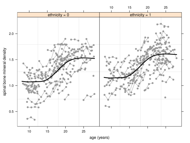
Figure 9: Plot obtained from execution of the last chunk of code in this Appendix.

References

Bachrach, L.K., Hastie, T., Wang, M.-C., Narasimhan, B. and Marcus, R. (1999). Bone mineral acquisition in healthy Asian, Hispanic, Black and Caucasian youth. A longitudinal study. Journal of Clinical Endocrinology and Metabolism, 84, 4702–12.

Berndt, E. R. (1991). The Practice of Econometrics: Classical and Contemporary. Reading, Massachusetts: Addison-Wesley.

Carroll, R.J., Ruppert, D., Stefanski, L.A. and Crainiceanu, C.M. (2006). Measurement Error in Nonlinear Models (Second Edition). Boca Raton, Florida: Chapman & Hall/CRC.

Cantoni, E. and Hastie, T. (2002). Degrees of freedom tests for smoothing splines. Biometrika, 89, 251–265.

Chaudhuri, P. & Marron, J.S. (1999). SiZer for exploration of structures in curves. Journal of the American Statistical Association, 94, 807–823.

Crainiceanu, C., Ruppert, D. and Wand, M.P. (2005). Bayesian analysis for penalized spline regression using WinBUGS. Journal of Statistical Software, Volume 14, Issue 14.

de Boor, C. (1978). A Practical Guide to Splines. Berlin: Springer-Verlag.

Denison, D.G.T., Holmes, C.C., Mallick, B.K. and Smith, A.F.M. (2002). Bayesian Methods for Nonlinear Classification and Regression. Chichester, UK: Wiley.

Eilers, P.H.C. and Marx, B.D. (1996). Flexible smoothing with B-splines and penalties (with discussion). Statistical Science, 11, 89–121.

Eubank, R.L. (1994). A simple smoothing spline. The American Statistician, 48, 103–106.

Eubank, R. L. (1999). Nonparametric Regression and Spline Smoothing. New York: Marcel Dekker.

Green, P.J. and Silverman, B.W. (1994). Nonparametric Regression and Generalized Linear Models. London: Chapman and Hall.

Gu, C. (2002). Smoothing Spline ANOVA Models. New York: Springer.

Hall, P. and Opsomer, J.D. (2005). Theory for penalised spline regression. Biometrika, 92, 105–118.

Hannig, J. and Marron, J.S. (2006). Advanced distribution theory for SiZer. Journal of the American Statistical Association, 101, 484–499.

Hastie, T. (2006). gam 0.97. R package. http://cran.r-project.org.

Hastie, T., Tibshirani, R. and Friedman, J. (2001). The Elements of Statistical Learning. New York: Springer-Verlag.

Luo, Z. and Wahba, G. (1997). Hybrid adaptive splines. Journal of the American Statistical Association, 92, 107–116.

Ngo, L. and Wand, M.P. (2003). Smoothing with mixed model software. Journal of Statistical Software, Volume 9, Issue 1.

Nussbaum, M. (1985). Spline smoothing in regression models and asymptotic efficiency in $L_{2}$. The Annals of Statistics, 13, 984–997.

Nychka, D. and Cummins, D.J. (1996). Comment on paper by Eilers and Marx. Statistical Science, 11, 104–105.

O’Sullivan, F. (1986). A statistical perspective on ill-posed inverse problems (with discussion). Statistical Science, 1, 505–527.

Ruppert, D. (2002). Selecting the number of knots for penalized splines. Journal of Computational and Graphical Statistics, 11, 735–757.

Ruppert, D., Wand, M. P. and Carroll, R.J. (2003). Semiparametric Regression. New York: Cambridge University Press.

Schoenberg, I.J. (1964). Spline functions and the problem of gradation. Proceedings of the National Academy of Sciences of the United States of America, 52, 947–950.

Solo, V. (2000). A simple derivation of the smoothing spline. The American Statistician, 54, 40–43.

Speed, T. (1991). Comment on paper by Robinson. Statistical Science, 6, 42–44.

Spiegelhalter, D., Thomas, A. and Best, N. (2000). WinBUGS Version 1.3 User Manual. www.hrc-bsu.cam.ac.uk/bugs.

Verbyla, A.P. (1994). Testing linearity in generalized linear models. Contributed Paper, 17th International Biometrics Conference, Hamilton, Canada., 177.

Wahba, G. (1990). Spline Models for Observational Data. Philadelphia: SIAM.

Wand, M. P. (2000). A comparison of regression spline smoothing procedures. Computational Statistics, 15, 443–462.

Welham, S.J., Cullis, B.R., Kenward, M.G. and Thompson, R. (2007). A comparison of mixed model splines for curve fitting. Australian and New Zealand Journal of Statistics, 49, 1–23.

Whittaker, E.T. and Robinson, G. (1967). The Newton-Cotes formulae of integration. Section 76 in The Calculus of Observations: A Treatise on Numerical Mathematics, 4th Edition. New York: Dover, pp.152–156.

Zhao, Y., Staudenmayer, J., Coull, B.A. and Wand, M.P. (2006). General design Bayesian generalized linear mixed models. Statistical Science, 21, 35–51.