The static spherically symmetric body in relativistic elasticity

Abstract

In this paper is discussed a class of static spherically symmetric solutions of the general relativistic elasticity equations. The main point of discussion is the comparison of two matter models given in terms of their stored energy functionals, i.e., the rule which gives the amount of energy stored in the system when it is deformed. Both functionals mimic (and for small deformations approximate) the classical Kirchhoff-St. Venant materials but differ in the strain variable used. We discuss the behavior of the systems for large deformations.

I Introduction

Classical elasticity is a phenomenological theory to describe the properties of solids. It is used heavily in applications such as structural mechanics and other engineering disciplines. This also explains the influence of classical elasticity in the formulation of the popular finite element method for the numerical solution of partial differential equations (see e.g. Hughes (2000)). While it is entirely sufficient to restrict oneself to a classical theory for bulk matter to describe every-day engineering problems it is nevertheless of conceptual interest to formulate a theory of elasticity which is compatible with the space-time structure established by Einstein’s theories of relativity.

The first attempts to merge elasticity with special relativity go back to the early 20th century and there have been several other formulations including Synge Synge (1959) and Rayner Rayner (1963). The most influential work, however, has been the paper by Carter and Quintana Carter and Quintana (1972) who formulated the geometric setting for the theory and derived the basic field equations. The theory has also been considered from a field theoretical point of view by Kijowski and Magli Kijowski and Magli (1992). Recently, the theory has been analyzed from the point of view of the initial value problem formulation by Beig and Schmidt Beig and Schmidt (2003). They showed that the field equations can be put into a first order symmetric hyperbolic form and they prove among other things that the Cauchy problem for the system is well-posed under various circumstances. Based on this formulation it is shown in Beig and Schmidt (2006) that there exist solutions of the elasticity equations in Newtonian theory and in special relativity describing elastic bodies in rigid rotation. In Andersson et al. (2006) it is proved that there exist solutions of the static elastic equations for sufficiently weak gravitational interaction. Losert Losert (2006) analyzes the case of a self-gravitating elastic spherical shell and shows existence of solutions in the Newtonian case.

In a series of papersKarlovini and Samuelsson (2003); Karlovini et al. (2004); Karlovini and Samuelsson (2004) Karlovini, Samuelsson and Zarroug adopt the formulation of Carter and Quintana to discuss spherically symmetric equilibrium configurations and their radial perturbations. They also present an exact static and spherically symmetric solution with constant energy density.

Our intention in this paper is to discuss two different equations of state in the static and spherically symmetric context with two different materials. In Beig and Schmidt (2003) the familiar Kirchhoff-St. Venant stored energy functional for hyper-elastic isotropic materials has been extended to the relativistic case. Recall that this functional is quadratic in the strain variable and contains the Lamé coefficients as two material constants. Kijowski and Magli in Kijowski and Magli (1992) use the same functional. However, they adopt a different definition for their strain variable which has a non-linear relationship to the strain used by Beig-Schmidt. Hence, this results in two different stored energy functionals which have the property that, by construction, they agree with the classical Kirchhoff-St.-Venant functional in the non-relativistic, small deformation limit.

The plan of the paper is as follows. In sec. II we provide the necessary background on the formulation of the theory of relativistic elasticity. The exposition follows that of Beig and Schmidt (2003). We present the two formulations by Beig-Schmidt and Kijowski-Magli and point out their differences. It turns out that the only difference is in the definition of the strain variable which accounts for the above mentioned different energy functionals.

In sec. III we specialize to the static and spherically symmetric case and derive the equations which govern this situation. We show that this system of equations has a unique smooth solution once the central compression of the body has been specified.

Sec. IV is devoted to a study of various models. In order to compare the two energy functionals we consider various scenarios. We discuss a solid aluminum sphere and a relativistic highly compact material similar to the nucleonic matter inside a neutron star, described with both theories as well as with the classical theory of elasticity. We also discuss how the choice of different natural states affects the solutions.

II Preliminaries

II.1 Relativistic Elasticity

The relativistic theory of elasticity in the form that we will use in this work has been described in Beig and Schmidt (2003). The kinematic structure of the theory can be formulated as follows. As the basic variable one considers a (smooth) map

$$f:\mathscr{M}\to\mathscr{B}$$ (1)

from space-time $(\mathscr{M},g)$ to a 3-dimensional manifold $\mathscr{B}$, the ’material manifold’ or ’body manifold’ or simply ‘the body’. This is a reference manifold which carries some additional structure which will be described later. The body manifold can be interpreted as the collection of all point-like constituents (baryons) of the actual body. Coordinates on $\mathscr{B}$ are labels for each individual ‘particle’ of the body. The map $f$ is a map from a 4-dimensional to a 3-dimensional manifold so its derivative $\mathrm{d}f$ must have a kernel. One requires that $F=\mathrm{d}f$ has maximal rank at each point so that this kernel has dimension one and is spanned by a unit vector field $u^{a}$. Using small Latin indices for tensors on $\mathscr{M}$ and capital Latin indices for tensors on $\mathscr{B}$, the derivative of $f$ may be written as $F^{A}_{a}=\partial_{a}f^{A}$. In local coordinates $(x^{a})$ on $\mathscr{M}$ and $(X^{A})$ on $\mathscr{B}$ the map $f$ is given by expressions of the form

$$X^{A}=f^{A}(x^{a}).$$ (2)

The dynamics of the theory is specified by a Lagrangian density $\rho$ which is regarded as a functional of $f$ and its first derivative $\mathrm{d}f$. In addition, it will depend on the metric $g$. Thus, the action may be written as

$$\mathscr{A}[f,\mathrm{d}f;g]=\int\rho[f,\mathrm{d}f;g]\,\sqrt{-\det g}\,d^{4}x.$$ (3)

The Euler-Lagrange equations for this action are

$$\mathscr{G}_{A}:=\frac{1}{\sqrt{-\det g}}\partial_{a}\left(\sqrt{-\det g}\frac{\partial\rho}{\partial(\partial_{a}f^{A})}\right)-\frac{\partial\rho}{\partial f^{A}}=0.$$ (4)

From the properties of $f$ one can already derive several useful consequences. Let $\Omega_{ABC}$ be a 3-form on $\mathscr{B}$. This 3-form can be interpreted as defining a measure on $\mathscr{B}$ which gives to each subset of $\mathscr{B}$ the number of particles contained in it. The pull-back of $\Omega_{ABC}$ to $\mathscr{M}$ along $f$ is a 3-form $\omega_{abc}$ on $\mathscr{M}$ which is dual to a vector field $\omega^{a}$. It is clear that this vector field spans the kernel of $f$ so that it must be proportional to $u^{a}$. Hence we have the formulas

$$\omega_{abc} =\Omega_{ABC}F^{A}_{a}F^{B}_{b}F^{C}_{c}=\epsilon_{abcd}\omega^{d},$$ (5)

$$\omega^{a} =nu^{a}=\frac{1}{6}\epsilon^{abcd}\omega_{bcd}.$$

The proportionality factor $n$ is interpreted as the number density of particles (baryon density) constituting the body in the state it acquires when embedded into space-time.

The energy-momentum tensor of the theory is defined as usual by the variation of the action with respect to the metric

$$T_{ab}=-2\frac{\partial\rho}{\partial g^{ab}}+\rho g_{ab}.$$ (6)

A consequence of the diffeomorphism invariance of the Lagrangian is (see Beig and Schmidt (2003)) that

$$\nabla_{b}T^{b}{}_{a}=\mathscr{G}_{A}F^{A}_{a}$$ (7)

i.e., that the elastic field equations are satisfied if and only if the energy-momentum tensor is divergence free. This is not necessarily the case in other field theories, such as e.g., for the Maxwell field.

The inverse metric $g^{ab}$ defines a contravariant, symmetric and positive definite 2-tensor $H^{AB}$ on the body by push-forward with the map $f$ (the minus sign is due to our signature)

$$H^{AB}=-g^{ab}F_{a}^{A}F_{b}^{B}.$$ (8)

This characterizes the current state of the body which can vary due to the space-time curvature. In order to describe the variation the conventional way is to compare the actual state with a reference state that is given a priori as a fixed structure on the body $\mathscr{B}$. This can be done by postulating the esxistence of a (positive definite) reference metric $\gamma_{AB}$ on the body manifold which characterizes a ‘natural’ state of the body in which – by definition – there is no strain. The difference $E^{AB}=H^{AB}-\gamma^{AB}$ between $H^{AB}$ and the inverse $\gamma^{AB}$ provides a measure of the ‘size’ of the strain on the body. Equivalently, one may use the linear map $\mathscr{E}=E^{A}{}_{B}=H^{A}{}_{B}-\delta^{A}_{B}$ obtained by lowering an index on $E^{AB}$ with $\gamma_{AB}$.

Writing $\rho=ne$ where $e$ is the energy per particle then the second Piola-Kirchhoff stress tensor is obtained as the derivative

$$\tau_{AB}=2\frac{\partial e}{\partial H^{AB}}.$$ (9)

Thus, specifying $e$ as a function of the strain provides the stress-strain relation i.e., the equation of state for the material under consideration. If the stress tensor $\tau_{AB}$ does not vanish in the natural state in which there is no strain then one talks about a pre-stressed state, otherwise the state is called stress-free or relaxed. We will be concerned only with a relaxed state. Thus, the energy density has a minimum in the natural state. For most applications it is enough to assume that the energy density is at most quadratic in the strain and we will do so here. Invariance under coordinate transformations in the body implies that it can depend only on the scalar invariants of $\mathscr{E}$ and since we are in three dimensions those invariants which are at most quadratic in $\mathscr{E}$ are $\mathop{\mathrm{Tr}}\nolimits\mathscr{E}$ and $\mathop{\mathrm{Tr}}\nolimits(\mathscr{E}^{2})$. Thus, the energy density can be written as

$$\rho =nm\left(1+\frac{1}{8}\left\{p\mathop{\mathrm{Tr}}\nolimits(\mathscr{E}^{2})+q(\mathop{\mathrm{Tr}}\nolimits\mathscr{E})^{2}\right\}\right)$$

$$=nm\left(1+\frac{1}{8}\left\{p(H^{AB}H_{AB}-2H^{A}{}_{A}+3)+q(H^{A}{}_{A}-3)^{2}\right\}\right)$$

where $m$ is the rest mass of a particle and $p$ and $q$ are constants. This is the stored energy functional which is assumed in Beig and Schmidt (2003). It describes the so-called Kirchhoff-St. Venant materials. When we refer below to the Beig-Schmidt (BS) formulation we mean the use of this stored energy functional.

The fact that there exists a metric on the body implies that there are now two 3-forms available: the 3-form $\Omega_{ABC}$ which gives the number of particles in each sub-domain of the body and the volume form $V_{ABC}$ induced by $\gamma_{AB}$ which gives the volume of the sub-domain. Since the two forms must be proportional we have

$$\Omega_{ABC}=n_{0}V_{ABC},$$ (10)

thus defining the particle density $n_{0}$ in the natural state. This can be used to define the mass density $\rho_{0}=mn_{0}$ in the natural state. Using the ‘natural’ particle density $n_{0}$ we can obtain the following formula

$$\omega_{abc}=\Omega_{ABC}F^{A}_{a}F^{B}_{b}F^{C}_{c}=n_{0}V_{ABC}F^{A}_{a}F^{B}_{b}F^{C}_{c}=n\epsilon_{abcd}u^{d}=n\epsilon_{abc}.$$ (11)

In local coordinates where $\Omega_{ABC}\doteq\sqrt{\det{\gamma}}\;d^{3}X$ and $\epsilon_{abc}\doteq\sqrt{-\det{h}}\;d^{3}x$ with $h_{ab}=g_{ab}-u_{a}u_{b}$, we have

$$n_{0}\sqrt{\det{\gamma}}\det{F}=n\sqrt{-\det{h}}.$$ (12)

II.2 The Kijowski-Magli strain

The main difference between the Beig-Schmidt Beig and Schmidt (2003) and Kijowski-Magli Kijowski and Magli (1992) formulations is the choice of the variable which measures the deformation. Beig-Schmidt use the difference between the actual and the relaxed metrics on the body while Kijowski-Magli use a logarithmic variable. They claim that this variable has better behavior when large deformations are studied.

With our choice of conventions and notation this variable is

$$S_{a}{}^{b}=-\frac{1}{2}\log(u_{a}u^{b}-\gamma_{a}{}^{b}),$$ (13)

where $\gamma_{ab}=F_{a}^{A}F_{b}^{B}\gamma_{AB}$ is the pull-back of the reference metric on $\mathscr{B}$ to the space-time. Note, that $\gamma_{ab}$ is positive definite so that the tensor inside the parentheses has only positive eigenvalues and the logarithm is well-defined.

Kijowski-Magli write down an action functional in terms of this variable. As before, the scalar character of the action implies that it can depend only on the scalar invariants of $S$ and Kijowski-Magli assume that it is at most quadratic in $S$. They introduce the invariants

$$\alpha=\mathop{\mathrm{Tr}}\nolimits S,\qquad\beta=\frac{1}{2}\mathop{\mathrm{Tr}}\nolimits\tilde{S}^{2}$$ (14)

where $\tilde{S}$ is the trace-free part of $S$. Then, they write the action in the form

$$\mathscr{A}=\int n\left(m+\frac{1}{2}A\alpha^{2}+B\beta\right)\;\sqrt{-\det g}\,\mathrm{d}^{4}x.$$ (15)

Here, we have adapted the formula of Kijowski-Magli somewhat because we use the particle density $n$ instead of the matter density and consequently we have to interpret $e$ as the energy per particle. When we refer to the Kijowski-Magli (KM) formulation we mean the use of this stored energy functional.

When deriving the equations of motion Kijowski and Magli use familiar techniques from Lagrangian field theory. However, their energy-momentum tensor is the canonical one and not the dynamical (symmetric) one which is obtained by varying the action with respect to the metric (see Szabados (2004) for a thorough discussion of this difference). Since we are using the latter tensor we cannot simply take over the expression of Kijowski-Magli. Instead, we need to derive this energy-momentum tensor explicitly as given in appendix A. We obtain

$$T_{ab}=\rho\,u_{a}u_{b}+n\alpha Ah_{ab}+nB\tilde{S}_{ab}.$$ (16)

II.3 Comparison of the two formulations

In this section we want to compare the two presented formulations of relativistic elasticity. We establish that they agree on the linearized level and show how they differ for large deformations. In order to compare these two formulations we introduce the following variable which measures the deformation from a given state

$$\epsilon_{a}{}^{b}=-\left(h_{ac}+\gamma_{ac}\right)h^{cb}=-h_{a}{}^{b}-\gamma_{a}{}^{b}.$$

In terms of $\epsilon_{a}{}^{b}$ we can write the KM deformation tensor in the form

$$S=-\frac{1}{2}\log(1+\epsilon).$$

The BS deformation is $E^{AB}=H^{AB}-\gamma^{AB}$. We can relate these two difference deformation variables by the following computation

$$E_{ab} =F^{A}_{a}F^{B}_{b}E_{AB}=-h^{cd}F^{A}_{a}F^{B}_{b}\gamma_{AC}\gamma_{BD}F^{D}_{d}F^{C}_{c}-\gamma_{AC}\gamma_{BD}\gamma^{CD}$$ (17)

$$=-\gamma_{ac}(\gamma_{bd}+h_{bd})h^{cd}=\gamma_{ac}\epsilon_{b}{}^{c}.$$

It follows that $E_{A}{}^{A}=(H^{AB}-\gamma^{AB})\gamma_{AB}=\epsilon_{ab}h^{ab}=\epsilon_{a}{}^{a}$ and also $E_{AB}E^{AB}=\epsilon_{ab}\epsilon^{ab}$. Thus, the BS-energy density takes the form

$$\rho_{BS}=nm\left(1+\frac{1}{8}\left\{p\epsilon_{ab}\epsilon^{ab}+q(\epsilon_{a}{}^{a})^{2}\right\}\right).$$

The KM variables $\alpha$ and $\beta$ can be expressed in terms of $\epsilon$ as well. Thus, e.g., $\alpha$ becomes

$$\alpha=-\frac{1}{2}\log\det(1+\epsilon)$$

and, similarly, $\beta$ can be expressed as before in terms of $S$ and hence in terms of $\epsilon$. In order to connect with the BS formulation we expand the energy density up to quadratic terms in $\epsilon$. For the expansion of $\alpha$ and $\beta$ we find

$$S_{a}{}^{b}\approx-\frac{1}{2}\epsilon_{a}{}^{b},\qquad\alpha\approx-\frac{1}{2}\epsilon_{a}{}^{a},\qquad\beta\approx\frac{1}{8}\epsilon_{ab}\epsilon^{ab}-\frac{1}{24}(\epsilon_{a}{}^{a})^{2},$$

so that the energy density of Kijowski-Magli up to second order in $\epsilon$ is

$$\rho_{KM}=n(m+\frac{1}{2}A\alpha^{2}+B\beta)\approx n\left(m+\frac{A}{8}\left(\epsilon_{a}{}^{a}\right)^{2}+\frac{B}{8}\epsilon_{ab}\epsilon^{ab}-\frac{B}{24}(\epsilon_{a}{}^{a})^{2}\right).$$

The expressions for the energy density in the two formulations agree in this approximation if we put

$$mp=B,\qquad mq=A-\frac{1}{3}B.$$

The coefficients in front of the quadratic terms can be related to the classical elastic constants. Introducing the number density $n_{0}$ in the natural state one defines the Lamé coefficients $\lambda=n_{0}mq$ and $2\mu=n_{0}mp$. Then, $n_{0}mA$ becomes the bulk modulus $K$ while $\mu$ is the shear modulus of the material.

Under these circumstances the energy-momentum tensor is given up to first order terms in $\epsilon_{ab}$ by

$$T_{ab}=\frac{n}{n_{0}}\rho_{0}\,u_{a}u_{b}-\frac{1}{2}\frac{n}{n_{0}}\left(2\mu\epsilon_{ab}-\lambda\epsilon_{c}{}^{c}\gamma_{ab}\right).$$

We contrast this with the exact energy-momentum tensors

BS: $$T_{ab}=\frac{n}{n_{0}}\rho_{0}\,u_{a}u_{b}+\frac{1}{2}\frac{n}{n_{0}}\left(2\mu\,\gamma_{ac}\epsilon^{c}{}_{b}+\lambda\,\epsilon_{c}{}^{c}\gamma_{ab}\right)$$ (18)

KM: $$T_{ab}=\frac{n}{n_{0}}\rho_{0}\,u_{a}u_{b}+\frac{n}{n_{0}}\left(2\mu\,h_{ab}\,\alpha+\lambda\,S_{ab}\right).$$ (19)

In the case of no deformation i.e., at a point where the body is in the natural state one has

$$\gamma_{ab}=-h_{ab}.$$

The BS-energy-momentum tensor reflects this relationship. It almost agrees with the linearized energy-momentum tensor except that $\gamma_{ab}$ appears instead of $-h_{ab}$. Both theories are quadratic in their respective deformation variables and therefore describe in some sense a Hookean theory in which stress and strain are proportional. However, the relationship between the two different strain variables is highly non-linear. While the two energy-momentum tensors agree for small strain they disagree heavily for large deformations. Similarly, the stored energy functionals which give the energy per particle as a function of strain are completely different in the two cases when viewed in terms of the strain variable $\epsilon_{a}{}^{b}$. Thus, the two formulations describe materials with different equations of state. Both materials behave like the usual Kirchhoff-St. Venant materials for small strain, but have a completely different behavior for large deformations. We want to explore some of the consequences of these differences in the remainder of this article.

In the KM formulation the strain variable is defined in terms of the difference tensors in space. This results in a term proportional to $h_{ab}$ in the energy-momentum tensor, i.e. a term which is isotropic in space. In contrast, in Beig and Schmidt (2003) is used the difference between the actual and the reference state on the body as the basic variable. This results in a term proportional to $\gamma_{ab}$, i.e., isotropic on the body. This has the consequence that it is much easier to describe a fluid as a special case of elastic material within the KM framework than in the BS case.

III Spherical Symmetry

Now we specialize to spherical symmetry. We take the space-time metric to be the general spherically symmetric and static metric

$$g=e^{2\eta}\,dt^{2}-e^{2\xi}\,dr^{2}-r^{2}\,(d\theta^{2}+\sin^{2}\theta\,d\phi^{2})$$ (20)

and we assume that the body metric $\gamma$ is spherically symmetric as well, i.e., when expressed in polar coordinates

$$\gamma_{AB}\doteq e^{2\xi_{0}}\,dR^{2}+R^{2}\,(d\Theta^{2}+\sin^{2}\Theta\,d\Phi^{2}).$$ (21)

Since the geometry at the origin should be regular we need $e^{2\xi_{0}}=1$ at the origin, i.e., $\xi_{0}(0)=0$. The function $\xi$ and $\eta$ depend on $r$ while $\xi_{0}$ depends only on $R$. The map $f:\mathscr{M}\to\mathscr{B}$ is assumed to be equivariant and thus without loss of generality it can be expressed as

$$f(r,\theta,\phi)=(F(r),\theta,\phi)$$ (22)

for some function $F(r)$ with $F(0)=0$. Then, the deformation gradient is given as

$$F^{A}_{a}\doteq F^{\prime}\mathrm{d}r\otimes\partial_{R}+d\theta\otimes\partial_{\Theta}+d\phi\otimes\partial_{\Phi}.$$ (23)

Clearly, because of staticity we must have $u^{a}\doteq e^{-\eta}\partial_{t}$ and from (12)

$$\frac{n}{n_{0}}=F^{\prime}\frac{e^{\xi_{0}}F^{2}\sin\theta}{e^{\xi}r^{2}\sin\theta}=F^{\prime}e^{\xi_{0}-\xi}\frac{F^{2}}{r^{2}}.$$ (24)

The pull-back $\gamma_{ab}$ of the reference metric on $\mathscr{B}$ is

$$\gamma_{ab}\doteq(e^{\xi_{0}}F^{\prime})^{2}dr^{2}+F^{2}\,(d\theta^{2}+\sin^{2}\theta\,d\phi^{2})$$ (25)

With these formulas and the abbreviations $x=F^{\prime}e^{-(\xi-\xi_{0})}$ and $y=F/r$ we can compute the deformation tensor

$$\epsilon_{a}{}^{b}\doteq\left(x^{2}-1\right)dr\otimes\partial_{r}+\left(y^{2}-1\right)\,(d\theta\otimes\partial_{\theta}+d\phi\otimes\partial_{\phi})$$ (26)

Using this variable and the formulas (18) and (19) we can find the energy-momentum tensors in both cases. They are given explicitly in the appendix B.

III.1 The equations

The Einstein equations in the spherically symmetric and static case are well known, see e.g. Wald (1984). They are

$$G_{0}{}^{0} =e^{-2\xi}\left\{\frac{1}{r^{2}}\left(1-e^{2\xi}\right)-\frac{2}{r}\xi^{\prime}\right\}=-8\pi\,\rho,$$ (27)

$$G_{1}{}^{1} =e^{-2\xi}\left\{\frac{1}{r^{2}}\left(1-e^{2\xi}\right)+\frac{2}{r}\eta^{\prime}\right\}=8\pi\,P,$$ (28)

$$G_{2}{}^{2} =e^{-2\xi}\left\{\eta^{\prime\prime}+(\eta^{\prime})^{2}-\eta^{\prime}\xi^{\prime}-\frac{1}{r}\left(\eta^{\prime}-\xi^{\prime}\right)\right\}=8\pi\,Q,$$ (29)

where we have put $T_{0}{}^{0}=\rho$, $P=-T_{1}{}^{1}$ and $Q=-T_{2}{}^{2}$. These are three equations for the unknown functions $\xi$, $\eta$ and $f$ (the function $\xi_{0}$ which specifies the reference metric is considered as given). A consequence of the Einstein equations is that the divergence of the energy-momentum tensor vanishes identically

$$\nabla_{a}T^{a}{}_{b}=0.$$ (30)

Under the current conditions this equation has only one non-trivial component

$$P^{\prime}+\eta^{\prime}(\rho+P)+\frac{2}{r}(P-Q)=0.$$ (31)

In order to obtain a useful system one replaces the equation (29) by (31). Furthermore, one integrates (27) by introducing the mass function

$$M(r)=4\pi\int_{0}^{r}\rho\bar{r}^{2}\,d\bar{r}$$ (32)

or, equivalently, the mean density $w=M(r)/r^{3}$ to obtain

$$e^{-2\xi}=1-2r^{2}w(r).$$ (33)

Inserting this into (28) one can solve for $\eta^{\prime}$ and insert this into (31). Then the following system of equations is obtained

$$rw^{\prime} =-3w+4\pi\rho,$$ (34)

$$r\eta^{\prime} =r^{2}\frac{4\pi P+w}{1-2r^{2}w},$$ (35)

$$rP^{\prime} =-r^{2}\frac{4\pi P+w}{1-2r^{2}w}(\rho+P)-2(P-Q).$$ (36)

This system is somewhat deceptive, because $\rho$, $P$ and $Q$ are functions of $F$ and its derivatives. Since they contain $F$ and $F^{\prime}$ in a non-linear way the third equation gives a complicated non-linear equation for $F^{\prime\prime}$. Equivalently, we will regard these functions as depending on $x$ and $y$ defined above. Then $P^{\prime}=P_{x}x^{\prime}+P_{y}y^{\prime}$. From their definition we get a relationship between $x$ and $y$

$$ry^{\prime}=xe^{\xi-\xi_{0}}-y$$ (37)

which can be used to substitute for $y^{\prime}$. With this preparation we now have the following final system of equations

$$rw^{\prime} =-3w+4\pi\rho,$$ (38)

$$ry^{\prime} =\frac{x}{\sqrt{1-2r^{2}w}}e^{-\xi_{0}}-y,$$

$$rx^{\prime} =\frac{P_{y}}{P_{x}}\left(y-\frac{x}{\sqrt{1-2r^{2}w}}e^{-\xi_{0}}\right)-r^{2}\frac{4\pi P+w}{1-2r^{2}w}\frac{\rho+P}{P_{x}}-\frac{2}{P_{x}}(P-Q).$$

Once a solution of this system is found we can obtain $\eta$ by integrating (35), $e^{-2\xi}$ is given by (33) and $F$ is found from the definition of $x$. The functions $\rho$, $P$ and $Q$ are specified by the choice of the elastic model as functions of $x$ and $y$, while $e^{-\xi_{0}}$ is any given function of $r$ characterizing the natural state of the body. It is only restricted by having the value of unity at the origin.

III.2 Behavior at the origin

The equations are singular at the origin $r=0$ and it is not a priori clear whether there exist regular solutions. If there are solutions which are bounded near the origin then they have specific values there which can be obtained from the system by putting $r=0$. Then the left hand sides vanish and from the right hand sides we get

$$w(0)=\frac{4\pi}{3}\rho(0),\quad y(0)=x(0)=:a,\quad P(0)=Q(0).$$ (39)

This shows us that the only free datum is the value $a$. It characterizes the volume change of the body at its center. Since the body should be compressed we assume that $a=\lim_{r\to 0}F(r)/r>1$. The initial value for $w$ can be computed from the expression of $\rho$ in terms of $x$ and $y$. The third condition states that in the center the radial and the tangential stresses should be equal and this is a condition on the matter model which cannot be influenced by specifying initial conditions. The fact that the central compression is enough to characterize a solution uniquely is physically reasonable and corresponds to the fact that a static fluid configuration is uniquely characterized by the central pressure.

In order to show that with these initial conditions there exist regular unique solutions we apply the theorem by Rendall and Schmidt Rendall and Schmidt (1991). The verification of the conditions necessary for that theorem are somewhat lengthy and we refer the reader to appendix C. It follows from this analysis that for a given value $a$ there exists a unique and smooth solution of the system of equations (38) in a neighborhood of the origin.

IV Numerical modeling of spherical elastic bodies

IV.1 The models

In the rest of this paper we solve the system (38) for several specific matter models. We consider two situations, a sphere consisting entirely of an ordinary material such as aluminum and a sphere which consists of material which resembles the neutron star crust. In both cases we choose the two different energy functionals corresponding to the BS and KM formulation, respectively. For aluminum we use the values $\rho_{0}=2720\,\mathrm{kg/m^{3}}$, $\lambda=63.3\,\mathrm{GPa}$ and $\mu=25\,\mathrm{GPa}$.

For the neutron star matter we follow the presentation in Haensel (2001) where the structure of the neutron star crust is described in detail. In the crust of a neutron star the density increases from the outer layer with $10^{6}\mathrm{g/cm^{3}}$ to the inner edge where the density is approximately $10^{14}\mathrm{g/cm^{3}}$. While the ground state of the matter is a lattice which has anisotropic elastic properties it is customary to approximate it by a homogeneous and isotropic elastic material. This material is under high pressure and hence it is much easier to shear it than to compress it. In fact, the material is often assumed to be incompressible. The shear modulus of the matter in the neutron star crust has been calculated in e.g. Strohmayer et al. (1991) and we use a value of $\mu=10^{26}\mathrm{Pa}$. The fact that the crust material is almost incompressible means that the bulk modulus $K$ is very large compared to the shear modulus and hence that also the Lamé coefficient $\lambda$ is very large. We take it here three orders of magnitude larger than the shear modulus, i.e., $\lambda=10^{29}\mathrm{Pa}$.

In the relativistic theories there is no canonical choice for the relaxed state of the body. While it seems natural to specify a flat metric on $\mathscr{B}$ this is not necessary. The choice of the relaxed metric has been discussed in the literature Kabobel (2001); Lukács (1977). We follow here a suggestion by Carter Carter according to which one can obtain the relaxed state by the following procedure. One assumes the body is heated up until it melts and then one lets it cool down until it solidifies again. Assuming that the fluid phase is an ideal fluid then the body settles in a state which can be described by a solution of the perfect fluid equations. Hence, besides a flat metric we also consider the spatial metric corresponding to an incompressible fluid with a constant density $\rho_{0}$, i.e, we put

$$e^{-2\xi_{0}}=1-\frac{8\pi}{3}\rho_{0}r^{2}.$$ (40)

As a third formulation we consider the classical non-relativistic theory of elasticity. The equations for the classical theory can be obtained from the relativistic equations as the Newtonian limit, see Beig and Schmidt (2003). The difference to the relativistic equations is that one puts $\xi=\xi_{0}=0$, so that $x=F^{\prime}$. Furthermore, eq. (31) is replaced by

$$P^{\prime}+\eta^{\prime}\rho+\frac{2}{r}(P-Q)=0,$$ (41)

where $\eta^{\prime}$ is the gravitational force, determined from the equation

$$\eta^{\prime}=\frac{M(r)}{r^{2}}=rw.$$ (42)

The stress components $P$ and $Q$ have the same functional form in terms of $x$ and $y$ as those for the BS-energy-momentum tensor, while $\rho$ is the mass density in the actual state, given by $\rho=\frac{n}{n_{0}}\rho_{0}=xy^{2}\rho_{0}$.

Hence, the non-relativistic system is

$$rw^{\prime} =-3w+4\pi\rho,$$ (43)

$$ry^{\prime} =x-y,$$

$$rx^{\prime} =\frac{P_{y}}{P_{x}}\left(y-x\right)-\frac{r^{2}}{P_{x}}w\rho-\frac{2}{P_{x}}(P-Q).$$

All the numerical solutions have been obtained using the Runge-Kutta ODE solver suite provided in MATLAB. The calculation is started with an initial value $a$ for $x(0)=y(0)$ which is used to calculate the initial value for $w(0)=4\pi/3\rho(0)$ from the energy-momentum tensor. The calculation stops when $P$ vanishes, indicating that the boundary of the body has been found.

IV.2 Numerical examples

We first study the aluminum sphere for the three formulations of elasticity. Clearly, for small values of the relative central compression $\delta=a-1$ the three formulations should be almost identical. We show in Fig. 1

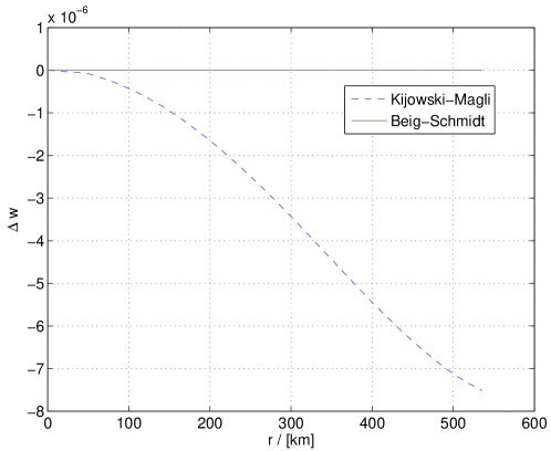
Figure 1: Relative difference between BS resp. KM and the classical solution for an aluminum sphere with relative central compression of $\delta=0.001$

the profile of the average density across the sphere for the three formulations for $\delta=0.001$. In this case we find a sphere with a radius of $535\,\mathrm{km}$ and a mass of $1.74\times 10^{12}\,\mathrm{kg}$. The figure shows the relative difference $\Delta w=(w-w_{N})/w_{N}$ between the classical solution $w_{N}$ and the BS and KM solutions $w$, respectively. The BS solution is indistinguishable from the classical solution, the maximum value of the relative difference being $6\times 10^{-13}$, while the KM solution already indicates its general property: the system is more tightly bound than in the classical or BS case. Still, in this situation of small relative central compression the maximal difference is only $7.5\times 10^{-6}$.

IV.2.1 Aluminum with BS-formulation

Let us now look at the BS model in more detail. The radial pressure is given by (58)

$$P=\frac{1}{2}(xy^{2})x^{2}\left((\lambda+2\mu)(x^{2}-1)+2\lambda(y^{2}-1)\right).$$ (44)

On the boundary of the body, this expression vanishes. This can happen either when $x=0$ or $y=0$ or if the term in parentheses vanishes. However, it follows from the equation for $y^{\prime}$ that as long as $x$ remains positive we have $y^{\prime}>0$ for $y=0$ so that $y$ cannot vanish before $x$ vanishes. Thus, on the boundary we have either $x=0$ or the pair $(x,y)$ lies on the ellipse defined by

$$(\lambda+2\mu)x^{2}+2\lambda y^{2}=3\lambda+2\mu.$$ (45)

In Fig. 2

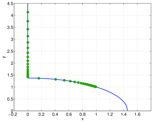
Figure 2: A sequence of pairs $(x,y)$ for relative central compressions $0.01\leq\delta\leq 4$

we show a sequence of such final pairs $(x,y)$ obtained from initial values $\delta$ in the interval $[0.01,4]$. Obviously, both cases discussed above can occur. For small relative central compressions the final pair $(x,y)$ lies on the ellipse and for increasing compression it moves towards the y-axis until it hits it for an initial value of $\delta\approx 0.585$. Then it moves along the y-axis for unlimited values of $y$. The vanishing of $x$ at the boundary means that the radial distance between two adjacent particles there becomes infinite, i.e. the body ruptures. Imagine a large elastic sphere without gravitational self-interaction being compressed so that the central compression is above the critical value. When gravity is switched on, the sphere will be divided into a central piece and a shell at the radius where $x$ vanishes.

The equation for $x^{\prime}$ in (38) shows that $x$ vanishes with an infinite negative slope because the leading term on the right hand side goes like $1/x$ near $x=0$. Thus, the solution becomes singular just at the boundary.

The two different cases just discussed can also be seen in the behavior of the mass-radius diagram in Fig. 3,

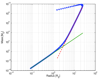
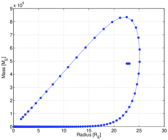
Figure 3: Double logarithmic (left) and linear (right) plot of the mass-radius diagram for BS aluminum spheres with relative central compression $\delta$, $\log_{10}\delta\in[-3,3]$, in units of the earth mass and radius, respectively. The solid line is $M\propto R^{3}$

where we display radius and mass of the aluminum spheres corresponding to relative central compressions $\delta\in[10^{-3},10^{3}]$. We plot it in double logarithmic and linear axes. The curve shows three different regimes, the classical one where $M\propto R^{3}$ (indicated by the solid line) and an ‘extreme’ regime where $M\propto R^{9}$, indicated by the dashed line and finally a ‘linear’ regime with $M\propto R$ where mass and radius decrease with increasing central compression. The cross indicates the configuration which is closest to the critical configuration where the radial strain $x$ vanishes. This mass-radius diagram should be compared with Figure 1 from Karlovini and Samuelsson (2004). The similarity of the qualitative behavior is obvious. Karlovini and Samuelsson argue that the branch from the maximal mass towards zero is unstable and we do find numerical indications of this here as well. Increasing the central compression beyond the value needed for the maximal mass configuration we observe that we can generate the smaller configurations up to a certain value of $\delta$ depending on the required precision. Beyond this value the solver suddenly settles to a solution which yields a configuration in the ‘eye’ inside the mass-radius diagram. This dot in fact contains nine different configurations. The location of the ‘eye’ is roughly at the mass resp. radius for which the radius resp. the mass are maximal on the curve. The behavior of this system close to the eye should be analyzed in much more detail using more accurate solution methods.

IV.2.2 Aluminum with KM formulation

In the formulation of Kijowski-Magli the radial pressure $P$ is given by (64)

$$P=(xy^{2})\left((\lambda+2\mu)\log x+2\lambda\log y\right).$$ (46)

As before, at the boundary we have either $x=0$ or

$$(\lambda+2\mu)\log x+2\lambda\log y=0,$$ (47)

the case $y=0$ being excluded as before. However, now, a final pair needs to lie on the curve defined by

$$y=\frac{1}{x^{\frac{1+\alpha}{2}}},\qquad\alpha=\frac{2\mu}{\lambda}>0.$$ (48)

This curve approaches the y-axis but never intersects it. This indicates that only the case when the final pair lies on the curve does occur. This is in fact confirmed in Fig. 4

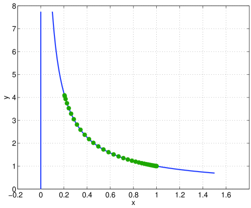
Figure 4: A sequence of pairs $(x,y)$ for relative central compressions $0.001\leq\delta\leq 25$

where we show the final pairs $(x,y)$ for aluminum spheres with relative central compression $\delta\in[0.001,25]$. While in the BS case the value of $y$ can grow arbitrarily, this is not the case here. In fact, the numerical investigations show that the exhibited value of $y\approx 4.1$ is the maximal value that $y$ can achieve. This behavior can be understood when we show the mass-radius diagram for KM aluminum spheres in Fig. 5

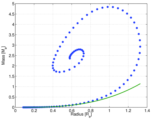
Figure 5: Mass-radius diagram for KM aluminum spheres with relative central compression $\delta$, $\log_{10}\delta\in[-3,3]$, in units of the earth mass and radius, respectively. The solid line indicates the curve $M\propto R^{3}$.

which shows a peculiar spiral. The maximal value of $y$ is reached at the same point as the maximal radius. Thus, it is not possible with the KM formulation to create arbitrarily large objects. There exists a maximal mass and a maximal radius for KM aluminum spheres achieved for different objects and there exists a region where a KM aluminum sphere of a given radius can have at least four different masses. It looks like the sequence converges to a limit point. We have not been able to prove this rigorously.

IV.2.3 The neutron star matter

We have also looked at an exotic material which is somewhat similar to the nucleonic matter that is assumed to be present in neutron stars. We show in Fig. 6

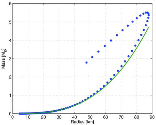
Figure 6: Mass-Radius diagram for BS neutron star like matter with relative central compression $\delta$, $\log_{10}\delta\in[-3,0.114]$, in units of solar mass and kilometers.

and in Fig. 7

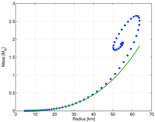
Figure 7: Mass-Radius diagram for KM neutron star like matter with relative central compression $\delta$, $\log_{10}\delta\in[-3,3]$, in units of solar mass and kilometers.

the mass-radius diagrams for the neutron star like matter distributions with the BS and KM stored energy functionals. In both cases the diagrams look qualitatively the same as those for aluminum except that the size of the configurations are orders of magnitudes different. In the KM case we find a spiral as before while in the BS case we have the ‘loop’ with a linearly decreasing branch. Again, this branch seems to be unstable and the final dot in the diagram is the last for which we could generate a configuration.

This shows that there is no qualitative difference in the behavior of aluminum and the exotic matter. This might change if one would use the high-pressure formulation developed by Carter and Quintana Carter and Quintana (1972).

IV.2.4 The role of the relaxed metric

As discussed above we employ two possible choices for the metric of the relaxed state of an elastic configuration. To compare the two different scenarios we compute configurations with the same relative central compression $\delta$ for values of $\delta$ between $10^{-3}$ and $1$ for the two energy functionals and the two possible materials. In Fig. 8

Figure 8: Maximal relative difference in the mean density $w$ between calculation with flat and curved metric for the relaxed state for given $\delta$ with $\log_{10}\delta\in[-3,0]$.

we show the behavior of the maximal absolute value

$$\frac{\Delta w}{w}=\max_{r}\left|\frac{w_{c}-w_{f}}{w_{f}}\right|$$

of the relative difference of the mean densities $w_{f}$ and $w_{c}$ for the flat and curved cases resp. as a function of $\delta$. Obviously, in the given range of $\delta$ the difference between the two configurations is almost negligible. The difference is larger for the exotic neutron star like material than for aluminum. The maximal difference is reached for the BS-energy functional with roughly 3%. For increasing $\delta$ the differences in three cases reach a maximum and afterwards decrease again. With increasing $\delta$ the elastic energy in the configuration increases with respect to the gravitational rest mass energy. Thus, the more the energy of the configuration is dominated by the elastic energy the smaller is the influence of the choice of a relaxed state. In any case, what can be learned from Fig. 8 is, that for practical purposes one can safely assume that the metric of the relaxed state is flat.

V Conclusion

We have discussed in this work the spherically symmetric body in relativistic elasticity for two different stored energy functionals. We find that the BS-functional corresponding to the classical Kirchhoff-St. Venant materials and the KM-functional have entirely different behavior for large deformations even though they agree for small deformations. The BS-functional gives rise to a mass-radius diagram which qualitatively is very similar to the one found by Karlovini and Samuelsson in Karlovini and Samuelsson (2004). They obtain this diagram for a stiff ultra-rigid equation of state in the Carter-Quintana high-pressure formulation. They find that the decreasing branch is unstable. We can confirm this numerically and we even see indications of another region of configurations. This is an indication that the BS-functional gives rise to an increasingly stiff equation of state quite in contrast to the KM-functional for which the equation of state becomes increasingly soft. The result of this softness can be seen in qualitatively very different behavior of the mass-radius diagram which shows a spiral which approaches a limit point for large deformations.

We looked at these functionals for two different materials, the ‘every day’ material aluminum and an artificial exotic material. While the sizes of the individual configurations are very different the qualitative behavior is very similar in both cases.

In order to analyze in more detail the features in these configurations and in particular the stability properties of the different branches of the mass-radius diagrams it might be advantageous to formulate the problem not as an initial value problem as we have done here. Instead of specifying the central compression and integrating outwards to (possibly) find the boundary of a configuration one would instead set up a boundary value problem on the body subject to the boundary conditions imposed by the symmetry requirements in the center and the vanishing of the radial pressure on the boundary. Steps in this direction have already been made by Losert Losert (2006).

Of course, our considerations are to a certain point academic because any real material will break at already quite moderate deformations compared to the ones we have used. But we feel that such questions of principle may shed some light on the differences between the various possible choices and therefore on the justification of assumptions made when relativistic elasticity is used for real problems.

Appendix A The symmetric energy-momentum tensor for the Kijowski-Magli action

The action for the Kijowski-Magli formulation of elasticity is (15)

$$\mathscr{A}=\int n\left(m+\frac{1}{2}A\alpha^{2}+B\beta\right)\;\sqrt{-\det g}\,\mathrm{d}^{4}x.$$

The energy-momentum tensor for this action is obtained (with our conventions) by variation of $\mathscr{A}$ with respect to the inverse metric

$$T_{ab}=-2\frac{\partial\rho}{\partial g^{ab}}+\rho g_{ab}.$$ (49)

The energy density $\rho$ is specified in terms of the variables $\alpha=S_{a}{}^{a}$ and $\beta=\frac{1}{2}S_{a}{}^{b}S_{b}{}^{a}-\frac{1}{6}(S_{a}{}^{a})^{2}$. The tensor $S_{a}{}^{b}$ was defined in (13)

$$S_{a}{}^{b}=-\frac{1}{2}\log\left(u_{a}u^{b}-\gamma_{a}{}^{b}\right).$$ (50)

To find the variation in these variables we first need to compute the variation with $g^{ab}$ in the tensor

$$K_{a}{}^{b}=u_{a}u^{b}-\gamma_{ac}g^{cb}.$$

We sketch the calculations here without going too much into the details. We start with the variation of (5) to obtain

$$\delta\omega^{d}=\frac{1}{2}\left(g_{ab}\delta g^{ab}\right)\,\omega^{d}.$$

Since, $n^{2}=g_{ab}\omega^{a}\omega^{b}$ we can now obtain the variation in $n$

$$2\frac{\delta n}{n}=h_{ab}\delta g^{ab}$$

and with $\omega^{a}=nu^{a}$ this yields the variation of $u^{b}$ and $u_{a}$

$$\delta u^{b}=\frac{1}{2}\left(u_{c}u_{d}\delta g^{cd}\right)u^{b},\qquad\delta u_{a}=\frac{1}{2}\left(u_{c}u_{d}\delta g^{cd}\right)u_{a}-g_{ac}u_{d}\delta g^{cd}.$$ (51)

From this we find

$$\delta(u_{a}u^{b})=\left(u_{c}u_{d}\delta g^{cd}\right)u_{a}u^{b}-g_{ac}u_{d}u^{b}\delta g^{cd}=-h_{ac}u_{d}u^{b}\delta g^{cd}$$ (52)

and hence

$$\delta K_{a}{}^{b}=-h_{ac}u_{d}u^{b}\delta g^{cd}-\gamma_{ac}\delta g^{cb}.$$ (53)

To compute $\delta\alpha$ we use the formula

$$\mathop{\mathrm{Tr}}\nolimits\log A=\log\det A$$ (54)

which follows from the corresponding well-known equation

$$\det\exp B=\exp\mathop{\mathrm{Tr}}\nolimits B,$$

valid for any matrix $B$. Thus, we have

$$\delta\alpha=-\frac{1}{2}\delta\mathop{\mathrm{Tr}}\nolimits\log K=-\frac{1}{2}\delta\log\det K=-\frac{1}{2}\frac{1}{\det K}\delta\det K.$$

Using the formula

$$\delta\det K=\det K\mathop{\mathrm{Tr}}\nolimits(K^{-1}\delta K)$$

we get the final result

$$\delta\alpha=-\frac{1}{2}\mathop{\mathrm{Tr}}\nolimits(K^{-1}\delta K)=-\frac{1}{2}(K^{-1})^{b}{}_{a}\delta K^{a}{}_{b}.$$ (55)

The variation of $\beta$ follows from the formula which can easily be derived

$$\delta\mathop{\mathrm{Tr}}\nolimits f(A)=\mathop{\mathrm{Tr}}\nolimits(f^{\prime}(A)\delta A).$$

We have $\beta=\frac{1}{2}\mathop{\mathrm{Tr}}\nolimits(S^{2})-\frac{1}{6}(\mathop{\mathrm{Tr}}\nolimits S)^{2}$ so we first compute

$$\delta\mathop{\mathrm{Tr}}\nolimits(S^{2})=\frac{1}{4}\delta\mathop{\mathrm{Tr}}\nolimits(\log(K)^{2})=\frac{1}{2}\mathop{\mathrm{Tr}}\nolimits(\log(K)K^{-1}\delta K)=-\mathop{\mathrm{Tr}}\nolimits(SK^{-1}\delta K)=-S_{a}{}^{b}(K^{-1})_{b}{}^{c}\delta K_{c}{}^{a}.$$

With this result we obtain

$$2\delta\beta=-\mathop{\mathrm{Tr}}\nolimits(SK^{-1}\delta K)+\frac{1}{3}\mathop{\mathrm{Tr}}\nolimits S\mathop{\mathrm{Tr}}\nolimits(K^{-1}\delta K)=-\mathop{\mathrm{Tr}}\nolimits(\tilde{S}K^{-1}\delta K).$$ (56)

These formulas can be simplified as follows. Using the fact that $S_{a}{}^{b}u^{a}=0$ and $K_{a}{}^{b}u^{a}=u^{b}$ we get

$$\begin{split}(K^{-1})_{a}{}^{b}\delta K_{b}{}^{a}&=-(K^{-1})_{a}{}^{b}(h_{bc}u_{d}u^{a}\delta g^{cd}+\gamma_{bc}\delta g^{ca})=-(K^{-1})_{a}{}^{b}\gamma_{bc}\delta g^{ca}=-(K^{-1})_{a}{}^{b}(u_{b}u_{c}-K_{bc})\delta g^{ca}\\ &=(-u_{a}u_{c}+g_{ac})\delta g^{ca}=h_{ab}\delta g^{ab}.\end{split}$$

Therefore, we have

$$\delta\alpha=-\frac{1}{2}h_{ab}\delta g^{ab}$$

and, similarly,

$$\delta\beta=-\frac{1}{2}\tilde{S}_{ab}\delta g^{ab}.$$

Now we can write down the variation of the energy

$$\delta\rho-\frac{\delta n}{n}\rho=n\left(A\alpha\delta\alpha+B\delta\beta\right)=-\frac{n}{2}\left[A\alpha h_{ab}+B\tilde{S}_{ab}\right]\delta g^{ab}.$$

With this in hand we can now finally write down the energy-momentum

$$T_{ab}=\rho\,u_{a}u_{b}+n\alpha Ah_{ab}+nB\tilde{S}_{ab}.$$

Appendix B Energy-momentum tensors

Using the abbreviations $x=F^{\prime}e^{-(\xi-\xi_{0})}$ and $y=F/r$ the energy-momentum tensor for the Beig-Schmidt theory is obtained from (18) using the expression (26) for $\epsilon_{a}{}^{b}$ in spherical symmetry. It has the following non-trivial components

$$T_{0}{}^{0}=\rho=xy^{2}\left(\rho_{0}+\frac{\mu}{4}\left\{(x^{2}-1)^{2}+2(y^{2}-1)^{2}\right\}+\frac{\lambda}{8}\left\{(x^{2}-1)+2(y^{2}-1)\right\}^{2}\right),$$ (57)

$$T_{1}{}^{1}=-P=-\frac{1}{2}(xy^{2})x^{2}\left((\lambda+2\mu)(x^{2}-1)+2\lambda(y^{2}-1)\right),$$ (58)

$$T_{2}{}^{2}=T_{3}{}^{3}=-Q=-\frac{1}{2}(xy^{2})y^{2}\left((2\lambda+2\mu)(y^{2}-1)+\lambda(x^{2}-1)\right).$$ (59)

The energy-momentum for the Kijowski-Magli formulation in spherical symmetry is obtained in a similar way from (19) once the tensor $S_{a}{}^{b}$ and its invariants $\alpha$ and $\beta$ are determined. Since $S=-\frac{1}{2}\log(1+\epsilon)$ and $\epsilon$ is diagonal in spherical symmetry this is straightforward:

$$S_{a}{}^{b}\doteq-(\log x)dr\otimes\partial_{r}-(\log y)\,(d\theta\otimes\partial_{\theta}+d\phi\otimes\partial_{\phi}).$$ (60)

Hence, we get

$$\alpha=-(\log x+2\log y),$$ (61)

and

$$\beta=\frac{1}{2}\left[(\log x)^{2}+2(\log y)^{2}\right]-\frac{1}{6}\left(\log x+2\log y\right)^{2}.$$ (62)

With these expressions we obtain the non-trivial components of the energy-momentum tensor

$$T_{0}{}^{0}=\rho=xy^{2}\left(\rho_{0}+\mu\left\{(\log x)^{2}+2(\log y)^{2}\right\}+\frac{\lambda}{2}\left\{\log x+2\log y\right\}^{2}\right),$$ (63)

$$T_{1}{}^{1}=-P=-(xy^{2})\left((\lambda+2\mu)\log x+2\lambda\log y\right),$$ (64)

$$T_{2}{}^{2}=T_{3}{}^{3}=-Q=-(xy^{2})\left((2\lambda+2\mu)\log y+\lambda\log x\right).$$ (65)

Appendix C Existence and Regularity of the solutions

Our goal here is to see whether the theorem by Rendall and Schmidt can be applied to our situation. For easy reference, we cite the theorem here

Theorem C.1 (Rendall and Schmidt)

Let $V$ be a finite dimensional vector space, $N:V\to V$ a linear map all of whose eigenvalues have positive real parts, and $G:V\times(-\epsilon,\epsilon)\to V$ and $g:(-\epsilon,\epsilon)\to V$ smooth maps, where $\epsilon>0$. Then, there exists $\delta<\epsilon$ and unique bounded $C^{1}$ function $u:(-\delta,0)\cup(0,\delta)\to V$ which satisfies the equation

$$s\frac{du}{ds}(s)+Nu(s)=sG(s,u(s))+g(s)$$ (66)

Moreover, $u$ extends to a smooth solution of (66) on $(-\delta,\delta)$. If $N$, $G$ and $g$ depend smoothly on a parameter $t$ and the eigenvalues of $N$ are distinct, then the solution depends smoothly on $t$.

To analyze the behavior of the equations at the center we follow the paper by Park Park (2000) who has found that the equations for the Kijowski-Magli allow smooth regular solutions. We need the same result for the equations coming from the formulation of Beig and Schmidt.

It is easy to see that a regular spherically symmetric scalar function $u(r)$ on a spherically symmetric space-time can smoothly be extended as an even function of $r$ to negative values of the radius. Thus, they depend smoothly on $s=r^{2}$ and their derivative at the center vanishes. Using $s$ as the independent parameter instead of $r$ our system (38) is

$$2sw^{\prime}+3w =4\pi\rho,$$ (67)

$$2sy^{\prime}+y =xf$$ (68)

$$2sP_{x}x^{\prime} =P_{y}(y-fx)-sf^{2}(w+4\pi P)(P+\rho)-2(P-Q),$$ (69)

where we have introduced $f=(1-2sw)^{-1/2}$. The solutions of this system will be regular only if $x(0)=y(0)=a$, $P(0)=Q(0)$ and $w(0)=4\pi/3\rho(0)$. Thus, we can write

$$x=a+sx_{1}(s),\qquad y=a+sy_{1}(s)$$

and derive equations for the functions $x_{1}(s)$ and $y_{1}(s)$. This yields the equations

$$2sw^{\prime}+3w =4\pi\rho,$$

$$2sy_{1}^{\prime}+3y_{1} =a\frac{f-1}{s}+x_{1}f,$$

$$2sx_{1}^{\prime}+2x_{1} =\frac{P_{y}}{P_{x}}\left(\frac{1-f}{s}a+(y_{1}-fx_{1})\right)-\frac{f^{2}}{P_{x}}(w+4\pi P)(P+\rho)-\frac{2}{s}\frac{P-Q}{P_{x}}.$$

The desired form is

$$2su^{\prime}+Nu=sG(u,s)+g(s).$$

The first equation is already in this form. In the second equation, the right hand side contains non-linear terms in $w$ (via $f$) but these terms have no factor $s$ in front. So we expand

$$f=\left(1-2sw\right)^{-1/2}=1+sw+\mathscr{O}(s^{2})$$

and get

$$2sy_{1}^{\prime}+3y_{1}=aw+x_{1}+\mathscr{O}(s).$$

Thus, this equation is in the desired form. Note, that it is not important for this analysis to know the $\mathscr{O}(s)$ exactly. It is enough to know that they are well behaved at the origin. The $\mathscr{O}(s)$ implies that they have the desired factor of $s$ in front.

The third equation is more difficult.Here, the right hand side of the equations contains non-linear terms in $w$, $x_{1}$ and $y_{1}$ through the dependence of $f$ and the functions $P$, $\rho$ and $Q$. Therefore, we have to expand the right hand side around $s=0$ and see whether we can isolate constant linear terms and non-linear terms proportional to $s$. So we write

$$P=P(x,y)=P(a+sx_{1},a+sy_{1})=P(a,a)+s(x_{1}P_{x}(a,a)+y_{1}P_{y}(a,a))+\mathscr{O}(s^{2})$$

and similarly for all the other functions on the right hand side. We write $P(a,a)=P^{0}$ and similarly for the other functions. First, we observe that we need to have

$$P^{0}-Q^{0}=0\qquad\text{and }\qquad P_{x}^{0}\neq 0$$

for the right hand side to be regular at all. Expanding the right hand side as indicated we get

$$2sx_{1}^{\prime}+4x_{1}+w\frac{P^{0}+\rho^{0}-aP_{y}^{0}}{P_{x}^{0}}+y_{1}\frac{P_{y}^{0}-2Q_{y}^{0}}{P_{x}^{0}}+x_{1}\frac{P_{y}^{0}-2Q_{x}^{0}}{P_{x}^{0}}=-4\pi P^{0}\frac{\rho^{0}+P^{0}}{P_{x}^{0}}+\mathscr{O}(s).$$

This is the desired form and we can collect the coefficients of the linear terms in the matrix $N$

$$N=\begin{pmatrix}3&0&0\\ -a&3&-1\\ \frac{P^{0}+\rho^{0}-aP_{y}^{0}}{P_{x}^{0}}&\frac{P_{y}^{0}-2Q_{y}^{0}}{P_{x}^{0}}&4+\frac{P_{y}^{0}-2Q_{x}^{0}}{P_{x}^{0}}\end{pmatrix}.$$

For the theorem to apply the eigenvalues of this matrix must be positive. This leads to the following conditions: if $P_{x}^{0}>0$ then also

$$6P_{x}^{0}+2P_{y}^{0}-3Q_{x}^{0}-Q_{y}^{0} >0,$$ (70)

$$7P_{x}^{0}+P_{y}^{0}-2Q_{x}^{0} >0,$$ (71)

while for $P_{x}^{0}<0$ the above expressions must also be negative.

Now we have reduced the question of regularity at the center to a condition for the energy functional which specifies the elastic properties of the material. It is straightforward to check that these conditions are satisfied for both the Beig-Schmidt and Kijowski-Magli stored energy functionals.

References

- Hughes (2000) T. J. R. Hughes, The finite element method (Dover, 2000).
- Synge (1959) J. L. Synge, Math. Z. 72, 82 (1959).
- Rayner (1963) C. B. Rayner, Proc. Roy. Soc. London A 272, 44 (1963).
- Carter and Quintana (1972) B. Carter and H. Quintana, Proc. Roy. Soc. London A 331, 57 (1972).
- Kijowski and Magli (1992) J. Kijowski and G. Magli, J. Geom. Phys. 9, 207 (1992).
- Beig and Schmidt (2003) R. Beig and B. G. Schmidt, Class. Quant. Grav. 20, 889 (2003).
- Beig and Schmidt (2006) R. Beig and B. G. Schmidt, Classical and Quantum Gravity (2006).
- Andersson et al. (2006) L. Andersson, R. Beig, and B. G. Schmidt, Static self-gravitating elastic bodies in einstein gravity (2006), URL http://arxiv.org/abs/gr-qc/0611108.
- Losert (2006) C. M. Losert, Static elastic shells in einsteinian and newtonian gravity (2006), URL http://arxiv.org/abs/gr-qc/0603103.
- Karlovini and Samuelsson (2003) M. Karlovini and L. Samuelsson, Classical and Quantum Gravity 20, 3613 (2003).
- Karlovini et al. (2004) M. Karlovini, L. Samuelsson, and M. Zarroug, Classical and Quantum Gravity 21, 1559 (2004).
- Karlovini and Samuelsson (2004) M. Karlovini and L. Samuelsson, Classical and Quantum Gravity 21, 4531 (2004).
- Szabados (2004) L. B. Szabados, Living Rev. Relativity 7 (2004), URL http://www.livingreviews.org/lrr-2004-4.
- Wald (1984) R. M. Wald, General Relativity (Chicago University Press, Chicago, 1984).
- Rendall and Schmidt (1991) A. Rendall and B. G. Schmidt, Class. Quant. Grav. 8, 985 (1991).
- Haensel (2001) P. Haensel, in Physics of Neutron Star Interiors, edited by D. Blaschke, N. Glendenning, and A. Sedrakian (2001), vol. 578, pp. 127–174.
- Strohmayer et al. (1991) T. Strohmayer, H. M. van Horn, S. Ogata, H. Iyetomi, and S. Ichimaru, Astrophysical Journal 375, 379 (1991).
- Kabobel (2001) A. Kabobel, Master’s thesis, Universität Tübingen (2001).
- Lukács (1977) B. Lukács, Nuovo Cimento B40, 169 (1977).
- (20) B. Carter, personal communication.
- Park (2000) J. Park, Gen. Rel. Grav. 32, 235 (2000), URL gr-qc/9810010.
- Penrose and Rindler (1984) R. Penrose and W. Rindler, Spinors and Spacetime, vol. 1 (Cambridge University Press, Cambridge, 1984).