Component sizes in networks with arbitrary degree distributions

Abstract

We give an exact solution for the complete distribution of component sizes in random networks with arbitrary degree distributions. The solution tells us the probability that a randomly chosen node belongs to a component of size $s$, for any $s$. We apply our results to networks with the three most commonly studied degree distributions—Poisson, exponential, and power-law—as well as to the calculation of cluster sizes for bond percolation on networks, which correspond to the sizes of outbreaks of SIR epidemic processes on the same networks. For the particular case of the power-law degree distribution, we show that the component size distribution itself follows a power law everywhere below the phase transition at which a giant component forms, but takes an exponential form when a giant component is present.

There has in recent years been considerable interest within the physics community in the properties of networks DM02 ; Newman03d ; NBW06 . Methods from physics, and particularly from statistical physics, have proved invaluable for understanding the structure and behavior of networked systems such as the Internet, the world wide web, metabolic networks, protein interaction networks, and social networks of interactions between people. In particular, by creating simple (and sometimes not-so-simple) models of network structure and formation, researchers have gained insight about the way networks behave as a function of the basic parameters governing their topology.

One of the most fundamental parameters of a network is its degree distribution. The degree of a node or vertex in a network is the number of edges connected to that vertex, and the frequency distribution of the degrees of vertices has been shown to have a profound influence on almost every aspect of network structure and function, including path lengths, clustering, robustness, centrality indices, spreading processes, and many others. Various network models have been used to illuminate the effects of the degree distribution, but perhaps the most widely studied, and certainly one of the simplest, is the so-called configuration model.

In the configuration model only the degrees of vertices are specified and nothing else; except for the constraint imposed by the degrees, connections between vertices are random. Equivalently, configuration model networks can be thought of as networks drawn uniformly at random from the set of all possible networks whose vertices have the specified degrees. One of the primary attractions of the configuration model is that many of its properties can be calculated exactly in the limit of large system size and for this reason it has become one of the fundamental tools for the quantitative understanding and study of networks. In 1995 Molloy and Reed MR95 gave an exact criterion for the existence of a giant component in the model and later also gave an expression for the expected size of that component MR98 . Newman, Strogatz, and Watts NSW01 gave additional expressions for a variety of other properties including number of vertices a given distance from a randomly chosen vertex, average path length in the giant component, and critical exponents near the transition at which the giant component appears, as well as generalizations of the model to bipartite and directed networks, and many further results have been presented since by a variety of authors.

One fundamental result that has been missing, however, is an expression for the sizes of components in the model other than the giant component. More specifically, if we choose a vertex at random from the network, what is the probability that it belongs to a component of a given size? As well as being a central structural property of the network, this distribution is directly related to important practical issues such as the distribution of the sizes of disease outbreaks for diseases spreading over contact networks Grassberger82 ; Newman02c .

At first sight, calculation of the component sizes appears difficult. One can derive equations that must be satisfied by the generating function for the distribution of component sizes NSW01 , but usually these equations cannot be solved. Here we show, however, that it is nonetheless possible to derive an explicit expression for the complete distribution of component sizes in the configuration model for general degree distribution. In particular, we show that it is possible to derive closed-form expressions for component sizes for the three most commonly studied degree distributions, the Poisson, exponential, and power-law distributions. We also show that the same techniques can be used to calculate the sizes of percolation clusters for percolation models on networks of arbitrary degree distribution, a development of some interest because of the close connection between percolation and epidemic processes. We explore this connection in the last part of the paper.

Let $p_{k}$ be the degree distribution of our network, i.e., the probability that a randomly chosen vertex has degree $k$. If rather than a vertex we choose an edge and follow it to the vertex at one of its ends, then the number of other edges emerging from that vertex follows a different distribution, the so-called excess degree distribution:

$$q_{k}={(k+1)p_{k+1}\over\langle k\rangle},$$ (1)

as shown in, for example, Ref. NSW01 . Here $\langle k\rangle=\sum_{k}kp_{k}$ is the average degree in the network.

It will be convenient to introduce the probability generating functions for the two distributions $p_{k}$ and $q_{k}$, thus:

$$g_{0}(z)=\sum_{k=0}^{\infty}p_{k}z^{k},\quad g_{1}(z)=\sum_{k=0}^{\infty}q_{k}z^{k}.$$ (2)

Many of our results are more easily expressed in terms of these generating functions than directly in terms of the degree distributions. It will also be convenient to note that

$$\langle k\rangle=g_{0}^{\prime}(1),\qquad g_{1}(z)={g_{0}^{\prime}(z)\over g_{0}^{\prime}(1)},$$ (3)

where we have made use of Eq. (1) in the second equality.

Now let us consider the distribution of the sizes of components in our network. Every vertex belongs to a component of size at least one (the vertex itself) and every edge connected to the vertex adds at least one more vertex to the component, and possibly many, if there are lots of other vertices that are reachable via that edge. Let us denote by $t$ the total number of vertices reachable via a particular edge, let the probability distribution of $t$ be $\rho_{t}$, and let the generating function for this distribution be $h_{1}(z)=\sum_{t}\rho_{t}z^{t}$.

The probability that a vertex of degree $k$ belongs to a component of size $s$ is the probability that the numbers of vertices reachable along each of its $k$ edges sum to $s-1$. This probability, which we will denote $P(s|k)$, is given by

$$P(s|k)=\sum_{t_{1}=1}^{\infty}\ldots\sum_{t_{k}=1}\delta\bigl{(}s-1,{\textstyle\sum_{m=1}^{k}t_{m}}\bigr{)}\prod_{m=1}^{k}\rho_{t_{m}},$$ (4)

where $\delta(i,j)$ is the Kronecker delta symbol. Then the probability $\pi_{s}$ of a randomly chosen vertex belonging to a component of size $s$ is $\pi_{s}=\sum_{k=0}^{\infty}p_{k}P(s|k)$ and the corresponding generating function is

$$h_{0}(z) =\sum_{s=1}^{\infty}\pi_{s}z^{s}=\sum_{s=1}^{\infty}\sum_{k=0}^{\infty}p_{k}P(s|k)z^{s}$$

$$=\sum_{k=0}^{\infty}p_{k}\sum_{s=1}^{\infty}z^{s}\sum_{t_{1}=1}^{\infty}\ldots\sum_{t_{k}=1}\delta\bigl{(}s-1,{\textstyle\sum_{m=1}^{k}t_{m}}\bigr{)}\prod_{m=1}^{k}\rho_{t_{m}}$$

$$=z\sum_{k=0}^{\infty}p_{k}\sum_{t_{1}=1}^{\infty}\ldots\sum_{t_{k}=1}z^{\sum_{m}t_{m}}\prod_{m=1}^{k}\rho_{t_{m}}$$

$$=z\sum_{k=0}^{\infty}p_{k}\biggl{[}\sum_{t=1}^{\infty}\rho_{t}z^{t}\biggr{]}^{k}=z\sum_{k=0}^{\infty}p_{k}[h_{1}(z)]^{k}.$$ (5)

But the final sum is simply the generating function $g_{0}(z)$, Eq. (2), evaluated at $h_{1}(z)$, and hence

$$h_{0}(z)=zg_{0}(h_{1}(z)).$$ (6)

By a similar argument the generating function $h_{1}(z)$ can be shown to satisfy

$$h_{1}(z)=zg_{1}(h_{1}(z)).$$ (7)

Between them, Eqs. (6) and (7) allow us, in principle, to calculate the entire distribution of cluster sizes in our network given the degree distribution $p_{k}$. Unfortunately, the self-consistent relation for $h_{1}(z)$, Eq. (7), is in most cases not solvable and hence we cannot calculate the value of the generating function. Surprisingly, however, we can still calculate the probabilities $\pi_{s}$.

Since every component is of size at least 1, the generating function $h_{0}(z)$ for the component sizes is of leading order $z$ (or higher) and hence contains an overall factor of $z$. Dividing out this factor and differentiating, we can write the probability of belonging to a cluster of size $s$ as

$$\pi_{s}={1\over(s-1)!}\biggl{[}{\mathrm{d}^{s-1}\over\mathrm{d}z^{s-1}}\biggl{(}{h_{0}(z)\over z}\biggr{)}\biggr{]}_{z=0}.$$ (8)

Using Eq. (6), this can also be written

$$\pi_{s} ={1\over(s-1)!}\biggl{[}{\mathrm{d}^{s-1}\over\mathrm{d}z^{s-1}}g_{0}(h_{1}(z))\biggr{]}_{z=0}$$

$$={1\over(s-1)!}\biggl{[}{\mathrm{d}^{s-2}\over\mathrm{d}z^{s-2}}\bigl{[}g_{0}^{\prime}(h_{1}(z))h_{1}^{\prime}(z)\bigr{]}\biggr{]}_{z=0}.$$ (9)

This expression can be rewritten using Cauchy’s formula for the $n$th derivative of a function,

$${\mathrm{d}^{n}\!f\over\mathrm{d}z^{n}}\biggr{|}_{z=z_{0}}={n!\over 2\pi\mathrm{i}}\oint{f(z)\over(z-z_{0})^{n+1}}\>\mathrm{d}z,$$ (10)

where the integral is around a contour that encloses $z_{0}$ in the complex plane but encloses no poles in $f(z)$. Applying this formula to Eq. (9) with $z_{0}=0$ we get

$$\pi_{s} ={1\over 2\pi\mathrm{i}(s-1)}\oint{g_{0}^{\prime}(h_{1}(z))\over z^{s-1}}\,{\mathrm{d}h_{1}\over\mathrm{d}z}\,\mathrm{d}z$$ (11a)

$$={\langle k\rangle\over 2\pi\mathrm{i}(s-1)}\oint{g_{1}(h_{1})\over z^{s-1}}\>\mathrm{d}h_{1},$$ (11b)

where we have used Eq. (3) to eliminate $g_{0}^{\prime}$ in favor of $g_{1}$. In (11a) we choose the contour to be an infinitesimal loop around the origin and, since $h_{1}(z)$ goes to zero as $z\to 0$, the contour in (11b) is then also an infinitesimal loop around the origin.

Now regarding $z$ as a function of $h_{1}$, rather than the other way around, we make use of (7) to eliminate $z$ and write

$$\pi_{s}={\langle k\rangle\over 2\pi\mathrm{i}(s-1)}\oint{\bigl{[}g_{1}(h_{1})\bigr{]}^{s}\over h_{1}^{s-1}}\>\mathrm{d}h_{1}.$$ (12)

Applying (10) again we then find that

$$\pi_{s}={\langle k\rangle\over(s-1)!}\biggl{[}{\mathrm{d}^{s-2}\over\mathrm{d}z^{s-2}}\bigl{[}g_{1}(z)\bigr{]}^{s}\biggr{]}_{z=0}.$$ (13)

(An alternative and equivalent way to derive this formula—although a less transparent one—would be to rearrange Eq. (7) to give $z$ as a function of $h_{1}$ and then apply the Lagrange inversion theorem AS65 to derive the Taylor expansion of $h_{1}$ or $h_{0}$. Indeed, Eqs. (8) to (13) are essentially a proof of a special case of the inversion theorem, as applied to the problem in hand.)

The only exception to Eq. (13) is for the case $s=1$, for which Eq. (11) gives $0/0$ and is therefore clearly incorrect. However, since the only way to belong to a component of size 1 is to have no connections to any other vertices, the probability $\pi_{1}$ is trivially equal to the probability of having degree zero:

$$\pi_{1}=p_{0}.$$ (14)

Between them, Eqs. (13) and (14) give the entire distribution of component sizes in terms of the degree distribution. They tell us explicitly the probability that a randomly chosen vertex belongs to a component of any given size $s$. For any specific choice of degree distribution, the application of Eq. (13) still requires us to perform the derivatives. Any finite number of derivatives can always be carried out exactly to give expressions for $\pi_{s}$ to finite order. It is also possible in some cases to find a general formula for any derivative and so derive a closed-form expression for $\pi_{s}$ for general $s$. In particular, it turns out to be possible, as we now show, to find such closed-form expressions for the three distributions most commonly studied in the literature, the Poisson, exponential, and power-law distributions.

A network in which edges are placed between vertices uniformly at random has a Poisson degree distribution

$$p_{k}=\mathrm{e}^{-c}{c^{k}\over k!},$$ (15)

where $c$ is the distribution mean. Such networks have been studied widely for some decades, most famously by Erdős and Rényi in the 1950s and 1960s ER59 ; ER60 . Given Eq. (15), it is straightforward to show that $g_{0}(z)=g_{1}(z)=\mathrm{e}^{c(z-1)}$ and the derivatives in Eq. (13) can be performed to give

$$\pi_{s}={\mathrm{e}^{-cs}(cs)^{s-1}\over s!}.$$ (16)

(The same expression also works for the special case $s=1$.) This expression for the component size distribution of the Poisson random graph has been derived in the past by a number of other methods—see for instance Bollobas01 —but it is a useful check on our methods to see it appear here as a special case of the more general formulation.

Few real-world networks, however, have Poisson degree distributions. Most have highly right-skewed distributions in which most vertices have low degree and a small number of “hubs” have higher degree. A number of networks, for example, are observed to have exponential degree distributions or distributions with an exponential tail. Examples include food webs, power grids, and some social networks ASBS00 ; DWM02a . Consider the exponential distribution $p_{k}=C\mathrm{e}^{-\lambda k}$, where $C$ is the appropriate normalizing constant. The generating functions in this case are

$$g_{0}(z)={\mathrm{e}^{\lambda}-1\over\mathrm{e}^{\lambda}-z},\qquad g_{1}(z)=\biggl{[}{\mathrm{e}^{\lambda}-1\over\mathrm{e}^{\lambda}-z}\biggr{]}^{2}.$$ (17)

Again the derivatives are straightforward to carry out and we find that

$${\mathrm{d}^{n}\over\mathrm{d}z^{n}}\bigl{[}g_{1}(z)\bigr{]}^{s}={(2s-1+n)!\over(2s-1)!}\,{\bigl{[}g_{1}(z)\bigr{]}^{s}\over(\mathrm{e}^{\lambda}-z)^{n}},$$ (18)

and hence

$$\pi_{s}={(3s-3)!\over(s-1)!(2s-1)!}\,\mathrm{e}^{-\lambda(s-1)}\bigl{(}1-\mathrm{e}^{-\lambda}\bigr{)}^{2s-1}.$$ (19)

Applying Stirling’s approximation for large $s$ we can show that this distribution behaves asymptotically as $\pi_{s}\sim s\mathrm{e}^{-\mu s}$, where $\mu=2\ln\bigl{[}\frac{3}{2}(1-\mathrm{e}^{-\lambda})\bigr{]}-\lambda$. Thus the component size distribution approximately follows an exponential law itself, although with an extra leading factor of $s$ and a different exponential constant.

However, perhaps the greatest amount of attention in recent years has been focused on networks that have power-law degree distributions of the form $p_{k}\propto k^{-\alpha}$ for some constant exponent $\alpha$ AJB99 ; FFF99 ; Kleinberg99b . A number of networks appear to follow this pattern, at least approximately, including the world wide web, the Internet, citation networks, and some social and biological networks DM02 . The observed value of the exponent typically lies in the range $2<\alpha<3$. Equivalently, we could say that the excess degree distribution $q_{k}$—which appears in the fundamental formula (13) via its generating function—follows a power law with exponent $\alpha-1$.

In fact, in essentially all cases, the observed power law holds only in the tail of the distribution; the distribution follows some other law for small degrees. This leaves us considerable latitude about the distribution we use in our calculations. Here we use a so-called Yule distribution for $q_{k}$, with a typical real-world value of $\alpha=2.5$ for the exponent:

$$q_{k}=C{\Gamma(k+\frac{1}{2})\over\Gamma(k+2)},$$ (20)

where $\Gamma(x)$ is the standard gamma function and $C$ is again a normalizing constant. It is straightforward to show (by Stirling’s approximation) that this distribution asymptotically follows a power law $q_{k}\sim k^{-3/2}$, which corresponds to a raw degree distribution $p_{k}\sim k^{-5/2}$. The Yule distribution appears in a number of contexts in the study of networks, particularly in the solutions of preferential attachment models that may explain the origin of power laws in some networks DMS00 ; KRL00 , and is considered by some to be the most natural choice of power-law form for discrete distributions. Employing this particular choice for our configuration model gives

$$g_{1}(z)={1\over 1+\sqrt{1-z}},$$ (21)

which in turn gives

$$\biggl{[}{\mathrm{d}^{n}\over\mathrm{d}z^{n}}\bigl{[}g_{1}(z)\bigr{]}^{s}\biggr{]}_{z=0} ={2^{-(2n+s)}\over(s-1)!}\times$$

$$\sum_{j=0}^{n-1}{(n-1+j)!(s+n-1-j)!\over j!(n-1-j)!}.$$ (22)

Setting $n=s-2$ and substituting into Eq. (13), we can complete the remaining sum to get

$$\pi_{s}=[1-\ln 2]^{-1}{(3s-5)!\over(s-1)!(2s-2)!}\,s\,2^{3-3s}.$$ (23)

In Fig. 1 we show the form of this distribution, along with those for the Poisson and exponential networks, Eqs. (16) and (19). Also shown in the figure are numerical results for the distributions of component sizes measured on computer generated networks with the same degree distributions. As the figure shows, there is excellent agreement between the simulations and the exact calculations.

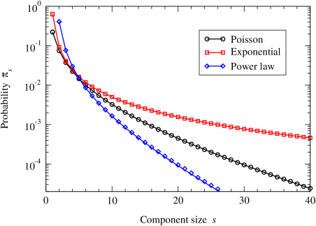
Figure 1: The distribution of component sizes in random graphs with Poisson ($c=1.5$), exponential ($\lambda=1$), and power-law ($\alpha=2.5$) degree distributions. Solid lines indicate the exact solutions derived in this paper. Points are the results of computer simulations for the same degree distributions. Each point is an average over $5000$ networks of $10^{6}$ vertices each. Error bars have been omitted, but are smaller than the data points in each case.

As with the exponential network, we can study the asymptotic form of the component size distribution (23) for the power-law network by making use of Stirling’s approximation. We find that in the limit of large $s$, $\pi_{s}\sim s^{3}\mathrm{e}^{-\nu s}$, where $\nu=5\ln 2-3\ln 3\simeq 0.1699\ldots$  Thus again we have an exponential tail to the distribution.

This last result is at first slightly surprising. One might imagine that the component size distribution should itself fall off as a power law or slower because the degree of a vertex provides a lower bound on the size of the component to which the vertex belongs—the fraction of vertices in components of size $s$ or greater must be at least as large as the fraction of vertices of degree $s$ or greater and hence the cumulative distribution of components falls off as slow or slower than the cumulative distribution of degrees.

So how is it possible that we have an exponential distribution of component sizes in the present case? The answer is that we are studying a network that has a giant component. Vertices not in the giant component—which make up almost all of the component size distribution—have a different degree distribution from the graph as a whole because the probability of not being in the giant component dwindles exponentially with increasing degree Newman02c . This creates an exponential cutoff for the degree distribution, and hence we are back to the situation we had for the exponential network, which gave an exponential component size distribution.

Thus in a power-law network we expect $\pi_{s}$ to have an exponential tail whenever there is a giant component in the network, but a power-law tail when there is no giant component. This contrasts with the case for essentially every other degree distribution, where we expect a power-law distribution of component sizes only precisely at the phase transition where the giant component forms; everywhere else we expect the distribution to fall off exponentially or faster NSW01 .

The methods described here can be extended to the calculation of cluster sizes for percolation processes on networks also. Of particular interest is the bond percolation process, whose cluster sizes give the distribution of outbreaks for a standard SIR epidemiological process on the same network Mollison77 ; Grassberger82 . Bond percolation can be framed in the same language as the calculation of component sizes above by considering the network formed by just the occupied edges. If the occupation probability is $\phi$, then it is straightforward to show Newman02c that the generating functions for the degree distribution and excess degree distribution of this latter network are $g_{0}(1-\phi+\phi z)$ and $g_{1}(1-\phi+\phi z)$, with $g_{0}$ and $g_{1}$ defined as before. Substituting into Eq. (13), we then find

$$\pi_{s}={\phi^{s-1}\langle k\rangle\over(s-1)!}\biggl{[}{\mathrm{d}^{s-2}\over\mathrm{d}z^{s-2}}\bigl{[}g_{1}(z)\bigr{]}^{s}\biggr{]}_{z=1-\phi}.$$ (24)

This result immediately implies that for all $\phi<1$ the distribution of cluster sizes falls off at least exponentially with increasing $s$. Thus, in the language of epidemiology, we will never see a power-law distribution of outbreak sizes, even if the network has a power-law degree distribution. This is, overall, good news: it implies that there will be no fat tail to the outbreak distribution and hence no unexpectedly large outbreaks, regardless of whether the network has a giant component.

To conclude, we have given an exact solution for the distribution of component sizes in random graphs with arbitrary degree distributions and applied it to networks with Poisson, exponential, and power-law distributed degrees. In the latter case we find that though the network has a power-law distribution of component sizes when there is no giant component, the distribution develops an exponential tail once a giant component appears. We have also applied our methods to bond percolation on networks, finding that percolation clusters always have an exponential tail to their distribution whenever the bond occupation probability is less than one.

The author thanks Cris Moore for useful conversations. This work was funded in part by the National Science Foundation under grant DMS–0405348 and by the Santa Fe Institute.

References

- (1) S. N. Dorogovtsev and J. F. F. Mendes, Evolution of networks. Advances in Physics 51, 1079–1187 (2002).
- (2) M. E. J. Newman, The structure and function of complex networks. SIAM Review 45, 167–256 (2003).
- (3) M. E. J. Newman, A.-L. Barabási, and D. J. Watts, The Structure and Dynamics of Networks. Princeton University Press, Princeton (2006).
- (4) M. Molloy and B. Reed, A critical point for random graphs with a given degree sequence. Random Structures and Algorithms 6, 161–179 (1995).
- (5) M. Molloy and B. Reed, The size of the giant component of a random graph with a given degree sequence. Combinatorics, Probability and Computing 7, 295–305 (1998).
- (6) M. E. J. Newman, S. H. Strogatz, and D. J. Watts, Random graphs with arbitrary degree distributions and their applications. Phys. Rev. E 64, 026118 (2001).
- (7) P. Grassberger, On the critical behavior of the general epidemic process and dynamical percolation. Math. Biosci. 63, 157–172 (1982).
- (8) M. E. J. Newman, Spread of epidemic disease on networks. Phys. Rev. E 66, 016128 (2002).
- (9) M. Abramowitz and I. A. Stegun (eds.), Handbook of Mathematical Functions. Dover Publishing, New York (1974).
- (10) P. Erdős and A. Rényi, On random graphs. Publicationes Mathematicae 6, 290–297 (1959).
- (11) P. Erdős and A. Rényi, On the evolution of random graphs. Publications of the Mathematical Institute of the Hungarian Academy of Sciences 5, 17–61 (1960).
- (12) B. Bollobás, Random Graphs. Academic Press, New York, 2nd edition (2001).
- (13) L. A. N. Amaral, A. Scala, M. Barthélémy, and H. E. Stanley, Classes of small-world networks. Proc. Natl. Acad. Sci. USA 97, 11149–11152 (2000).
- (14) J. A. Dunne, R. J. Williams, and N. D. Martinez, Food-web structure and network theory: The role of connectance and size. Proc. Natl. Acad. Sci. USA 99, 12917–12922 (2002).
- (15) R. Albert, H. Jeong, and A.-L. Barabási, Diameter of the world-wide web. Nature 401, 130–131 (1999).
- (16) M. Faloutsos, P. Faloutsos, and C. Faloutsos, On power-law relationships of the internet topology. Computer Communications Review 29, 251–262 (1999).
- (17) J. M. Kleinberg, S. R. Kumar, P. Raghavan, S. Rajagopalan, and A. Tomkins, The Web as a graph: Measurements, models and methods. In T. Asano, H. Imai, D. T. Lee, S.-I. Nakano, and T. Tokuyama (eds.), Proceedings of the 5th Annual International Conference on Combinatorics and Computing, number 1627 in Lecture Notes in Computer Science, pp. 1–18, Springer, Berlin (1999).
- (18) S. N. Dorogovtsev, J. F. F. Mendes, and A. N. Samukhin, Structure of growing networks with preferential linking. Phys. Rev. Lett. 85, 4633–4636 (2000).
- (19) P. L. Krapivsky, S. Redner, and F. Leyvraz, Connectivity of growing random networks. Phys. Rev. Lett. 85, 4629–4632 (2000).
- (20) D. Mollison, Spatial contact models for ecological and epidemic spread. Journal of the Royal Statistical Society B 39, 283–326 (1977).