[0707.0071] 1 The AWI mass for the three combinations of quark masses. The linear extrapolation to 𝑀_AWI=0 gives an additive mass renormalization 𝑀₀=0.0147⁢(3).

2+1 Flavor QCD simulated in the $\epsilon$ -regime in different topological sectors

P. Hasenfratz^a, D. Hierl^b, V. Maillart^a, F. Niedermayer^a, A. Schäfer^b, C. Weiermann^a and M. Weingart^a

^aInstitute for Theoretical Physics

University of Bern

Sidlerstrasse 5, CH-3012 Bern, Switzerland

^bInstitute for Theoretical Physics, University of Regensburg, D-93040 Regensburg, Germany

Abstract

We generated configurations with the parametrized fixed-point Dirac operator $D_{\mathrm{FP}}$ on a $(1.6\,\mathrm{fm})^{4}$ box at a lattice spacing $a=0.13\,\mathrm{fm}$ . We compare the distributions of the three lowest $k=1,2,3$ eigenvalues in the $\nu=0,1,2$ topological sectors with that of the Random Matrix Theory predictions. The ratios of expectation values of the lowest eigenvalues and the cumulative eigenvalue distributions are studied for all combinations of $k$ and $\nu$ . After including the finite size correction from one-loop chiral perturbation theory we obtained for the chiral condensate in the $\overline{\mathrm{MS}}$ scheme $[\Sigma(2\,\mathrm{GeV})]^{1/3}=0.239(11)\,\mathrm{GeV}$ , where the error is statistical only.

Spontaneous chiral symmetry breaking and the related existence of light Goldstone bosons is a basic feature of QCD. Chiral Perturbation Theory (ChPT) provides a systematic description of this physics in terms of a set of low energy constants which encode the related non-perturbative features of QCD. The method of low energy effective Lagrangians simplifies the calculations significantly [1, 2, 3, 4] and over the years ChPT became a refined powerful technique. Gasser and Leutwyler recognized very early, decades before the numerical calculations could attack such problems, that these constants can also be fixed using physical quantities which, presumably, will never be measured in real experiments. They can be studied, however, in lattice QCD.

The $\epsilon$ - regime [5, 6, 7, 8] describes physics close to the chiral limit in a box whose size is larger than the QCD scale. On the other hand, the size of the box relative to the Goldstone boson correlation length must be small. Under these conditions the Goldstone bosons, as opposed to other excitations, feel the effect of boundaries strongly. ChPT provides a powerful and systematic way to calculate the finite size corrections. A nice additional feature of the $\epsilon$ -regime is that Random Matrix Theory (RMT) [9] makes precise predictions for microscopic observables. RMT relates in particular the distribution of low-lying eigenvalues of the Dirac operator in different topological sectors to the chiral condensate.

The pioneering numerical works [10, 11, 12, 13, 14, 15, 16] in the $\epsilon$ -regime in quenched QCD suggested that this regime can be an excellent tool to study low-energy physics in QCD. The special problems of the $\epsilon$ -regime called for new numerical procedures [14, 15, 16, 17] which were first tested also in this approximation. Combining these numerical developments with the renormalization properties of the spectral density the work [18] present a state of the art analysis for the quark condensate and the first Leutwyler-Smilga sum rule in quenched QCD. The quenched approximation, however, tends to be singular in the chiral limit and it is expected that quenching is even more problematic here than in other cases [19].

Unfortunately, full QCD simulations are expensive. In addition, in the $\epsilon-$ regime the Dirac operator should have excellent chiral properties. The standard choice is the overlap Dirac operator [20] with a hybrid Monte Carlo algorithm.

The results in [21] reflect already the basic physics features of the $\epsilon$ -regime. The distribution of the low-lying eigenmodes could be fitted quite well to the RMT predictions and a reasonable value for the chiral condensate was obtained. These results are promising given the fact that the box was small ( $1.3\,\mathrm{fm}$ ), the quark mass was rather large ( $m_{q}\geq 40\,\mathrm{MeV}$ ) and the lattice was coarse ( $a=0.16\,\mathrm{fm}$ ). The results in a larger box of $1.5\,\mathrm{fm}$ and at smaller quark mass $m_{q}\approx 20\,\mathrm{MeV}$ obtained in [22] were consistent with those of [21].

The first serious simulation results in the $\epsilon$ -regime have been presented by the JLQCD group recently [23]. In that work $N_{f}=2$ QCD was simulated with overlap fermions (created with the Wilson kernel) on a lattice of size $1.8^{3}\times 3.6\,\mathrm{fm}^{4}$ with a resolution $a=0.11\,\mathrm{fm}$ obtained from $r_{0}$ . Different bare quark masses ( $am_{q}$ ) were considered in the range $0.110,\dots,0.020,0.002$ . The smallest quark mass (corresponding to $\approx 3\,\mathrm{MeV}$ ) was certainly small enough to reach the $\epsilon$ -regime. Hybrid Monte Carlo with overlap fermions has problems when the topological charge changes. To avoid this an action was used which prevented topology change and the whole run stayed in the $Q=0$ sector. The authors observed an overall good agreement with RMT. The fermion condensate, which is the only parameter to be fitted, was found to be $\Sigma(2\,\mathrm{GeV})^{1/3}=0.251(7)(11)\mathrm{GeV}$ in the $\overline{\mathrm{MS}}$ scheme.

Our work is based on the parametrized fixed-point (FP) action which has been tested in detail in quenched QCD [24]. The exact FP Dirac operator satisfies the Ginsparg-Wilson relation

D_{\mathrm{GW}}^{\dagger}+D_{\mathrm{GW}}=D_{\mathrm{GW}}^{\dagger}2RD_{\mathrm{GW}}\,,

(1)

where $R$ is a local operator and is trivial in Dirac space. The parametrized FP action has many gauge paths and involves a special smearing with projection to the gauge group $\mathrm{SU}(3)$ . As a consequence, hybrid Monte Carlo algorithms can not be used. In the work [25] we advised a partially global update with three nested accept/reject steps which can reach small quark masses even on coarse lattices. Several steps of this algorithm were developed in [26] using some earlier suggestions [27, 28, 29, 30]. All the three steps are preconditioned. Pieces of the quark determinant are switched on gradually in the order of their computational expenses. The largest and most fluctuating part of the determinant is coming from the ultraviolet modes. We reduce these fluctuations by calculating the trace of $D_{\mathrm{FP}}^{n},n=1,...,4$ [31, 32, 26]. The $\sim 100$ lowest-lying modes are calculated and subtracted. The determinant of the reduced and subtracted $D_{\mathrm{FP}}$ is calculated stochastically [33, 34, 35, 36]. For the determinant breakup we generalized the mass shifting method of [31]. For the strange quark we performed a root operation. Since the strange quark mass is not very small, we used a polynomial expansion to approximate this root operator. Recently we replaced the polynomial expansion by a rational approximation [37] which brought a $\approx 30\%$ performance gain in this part.

Due to the partial global updating procedure the algorithm, beyond a certain volume, scales with $V^{2}$ which constrains the size of lattices which can be considered. Due to the large number of subtracted low-lying modes, small quark mass is not a barrier.

We generated $\sim 4000$ configurations in the Markov chain on an $12^{4}$ lattice using the partially global algorithm discussed above. The distance between every second configurations in this chain is similar to that of two gauge configurations separated by a typical Metropolis gauge update sweep. We considered every tenth configurations from the Markov chain and performed the measurements on the remaining $\sim 400$ configurations. When calculating statistical errors we formed 20 bins and used the jackknife method.

We fixed the lattice spacing from the Sommer parameter [38] $r_{0}=0.49\,\mathrm{fm}$ and found $a=0.129(5)\,\mathrm{fm}$ . Our box has the size $(1.6\,\mathrm{fm})^{4}$ .

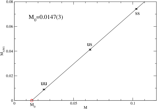
The Dirac operator $D_{\mathrm{FP}}$ has no exact chiral symmetry due to parametrization errors. As a consequence, the quark masses have an additive mass renormalization. The degenerate $u,\,d$ and the $s$ quark masses in the code are $M_{\mathrm{ud}}=0.025$ and $M_{\mathrm{s}}=0.103$ . The additive renormalization was measured following the steps described in [39] and has the value $M_{0}=0.0147(3)$ , as shown in Fig. 1. Subtracting the additive renormalization we get the bare masses $m_{\mathrm{ud}}=0.0103(3)$ and $m_{\mathrm{s}}=0.0883(3)$ which corresponds to $16\,\mathrm{MeV}$ and $137\,\mathrm{MeV}$ , respectively.

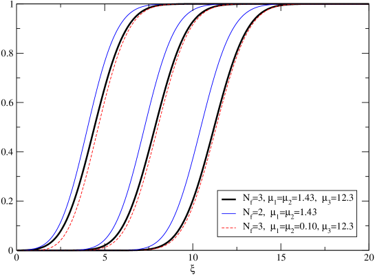
Refer to caption — Figure 1: The AWI mass for the three combinations of quark masses. The linear extrapolation to $M_{\mathrm{AWI}}=0$ gives an additive mass renormalization $M_{0}=0.0147(3)$ .

As we mentioned above, a simulation with lighter quark masses would not be more expensive. In our case, however, a smaller $m_{\mathrm{ud}}$ were not useful either. RMT predicts the probability distribution $p_{\nu k}(\xi_{\nu k})$ for the $k$ -th low-lying eigenvalue ( $k=1,2,\dots$ ) of the Dirac operator in the topological sector $\nu$ . Denoting the corresponding eigenvalues of the (continuum) Dirac operator by $i\alpha_{\nu k}$ , the variable $\xi_{\nu k}$ is related to the bare chiral condensate $\Sigma$ as $\xi_{\nu k}=\alpha_{\nu k}\Sigma V$ . Here V is the volume of the box. Fig. 2 shows the prediction of RMT for the cumulative distributions $\int^{\xi_{\nu k}}_{0}d\xi p_{\nu k}(\xi)\,$ for $\nu=0$ and $k=1,2,3$ . The distributions depend on $\mu_{i}=m_{i}\Sigma V$ where $m_{i}$ are the quark masses. Decreasing the $m_{\mathrm{ud}}$ mass by more than a factor 10 (at fixed $m_{\mathrm{s}}$ ) the cumulative distributions practically remain unchanged. On the other hand sending the strange quark mass to infinity (at fixed $m_{\mathrm{ud}}$ ) we land on a $N_{f}=2$ flavor theory with a visibly different distribution. The strange quark has a (modest) effect on our observables.

While the eigenvalues of the continuum Dirac operator lie on the imaginary axis the spectrum of lattice Dirac operators is more complicated. As it is well known, the spectrum of the Dirac operator satisfying the Ginsparg-Wilson relation with $2R=1$ lies on the circle $|\lambda-1|=1$ . In our case where $2R$ is different from 1, it is convenient to introduce the rescaled operator $\hat{D}_{\mathrm{GW}}=\sqrt{2R}D_{\mathrm{GW}}\sqrt{2R}$ , for which the $2R$ factor is eliminated in the GW relation, and the spectrum lies on the circle. (In fact, our operator $2R$ for the low-lying modes is effectively a constant close to 1 within a few percent.) To relate the eigenvalues on the GW circle to those appearing in the RMT (or in general, in continuum expressions) it is natural to use the stereographic projection

i\alpha=\frac{\lambda}{1-\lambda/2}\,.

(2)

As Fig. 3 shows, the low-lying eigenvalues of $D_{\mathrm{FP}}(m)$ (which we obtain during our simulation) are close but not exactly on the GW circle, hence we project them first horizontally onto the GW circle, and make the stereographic projection in the next step. This is justified by the observation that making a systematic GW improvement of $D_{\mathrm{FP}}$ towards $D_{\mathrm{GW}}$ the imaginary part of the eigenvalues stays practically constant – they move horizontally to the GW circle. The values of $\alpha$ obtained by this procedure are then compared with the RMT predictions.

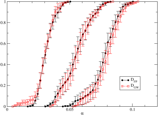
Having the probability distributions from RMT we can calculate the ratios $\langle\xi_{\nu k}\rangle/\langle\xi_{\nu^{\prime}k^{\prime}}\rangle$ , where the factor $\Sigma V$ cancels. These predictions are compared with the measured ratios in Fig. 4, where all the ratios in the topological sectors $\nu=1,2,3$ for the first three lowest eigenvalues are shown.

At this point we have to discuss the way we identify the topological sectors. According to the index theorem [40] one can identify the topological charge from the zero modes of a Ginsparg-Wilson Dirac operator. However, our $D_{\mathrm{FP}}$ has no exact chiral symmetry and has modes on the real axis. Occasionally, the real eigenvalue $\lambda$ might be even far from zero in which case the topological interpretation is uncertain. We note here that using an exact Ginsparg-Wilson operator (with kernel $D_{\mathrm{FP}}$ ) for measuring the topological charge is not a good solution to this problem. The overlap just projects most of the real eigenvalues to the point $\lambda=0$ . Following the intuitive picture that topology is related to extended objects we investigated the correlation between the inverse participation ratio (IPR) of the eigenvector having a real eigenvalue $\lambda$ and the value of $\lambda$ . Here IPR is given by $\sum_{x}\sum_{i=1}^{12}|\psi_{i}^{(\lambda)}(x)|^{4}$ for a normalized eigenvector $\psi^{(\lambda)}$ . The IPR is inversely proportional to the size of the effective support of the eigenfunction. As Fig. 5 shows, there is a strong correlation indeed. As $\lambda$ is moving away from zero, the IPR increases indicating that the wave function becomes more and more localized. Fig. 6 demonstrates that the real eigenvalues $\lambda(D_{\mathrm{FP}})$ are strongly concentrated in a small region close to zero. The histogram of $\lambda(D_{\mathrm{FP}})$ has a large, narrow peak followed by a long tail.

Fig. 7 shows the histogram of IPR for the real eigenmodes of $D_{\mathrm{FP}}$ . There is a strong, narrow peak which corresponds to extended real modes and a long tail corresponding to wave functions with smaller support.

For the questions we study in this paper it is not necessary to use a procedure which leaves the relative weights of the different topological sectors intact. (Due to the long autocorrelation time of the topological charge it would be anyhow difficult to control these weights.) We introduce therefore a cut above which the real eigenvalues are discarded. This cut must be sufficiently small to allow for a good identification of the topological charge, but large enough to allow for a reasonable number of configurations in each sectors we want to investigate. The cut should be smaller than the spectral gap (for the spectrum see Fig. 8), otherwise the effect of topology will be strongly reduced. We introduced a cut of size 0.03 which is approximately equal to the minimal gap in the $\nu=1$ sector. We accepted a real eigenvalue $\lambda$ as a sign of topology if $\lambda<0.03$ . This cut splits our sample of 414 configurations into 328, 51 and 35 configurations for the $\nu=0,1,2$ sectors, respectively. This cut corresponds also to the end of the peak of the IPR distribution shown in Fig. 7.

Fig. 9 compares the cumulative distributions of the first three eigenvalues in the $\nu=0$ topological sector obtained using the overlap improved fixed-point Dirac operator $D_{\mathrm{GW}}$ vs. $D_{\mathrm{FP}}$ in the measurement. The distributions are very similar showing that the two operators are close to each other. The $k=1$ distribution from $D_{\mathrm{GW}}$ has a tail at small eigenvalues (i.e. has a smaller gap than $D_{\mathrm{FP}}$ ) demonstrating a systematic error one obtains when using different Dirac operators for the generation of the configurations and for the measurements: the small eigenvalues are less effectively suppressed.

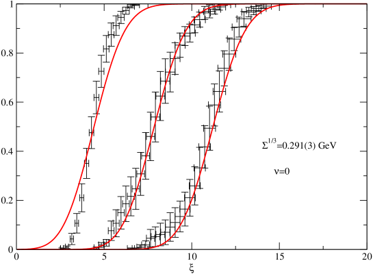
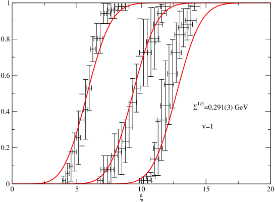
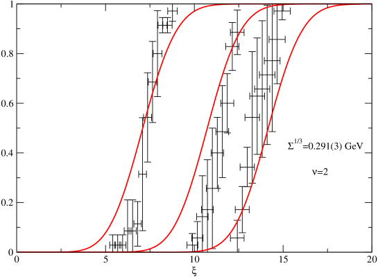
In Figs. 10, 11, 12 the cumulative distributions of the $D_{\mathrm{FP}}$ operator are compared with RMT for the $\nu=0,1,2$ topological sectors. The only matching parameter is the bare condensate $\Sigma$ which enters the RMT predictions through $\mu_{i}=m_{i}\Sigma V$ and in $\alpha\Sigma V$ . We obtained the result for this bare quantity $\Sigma^{1/3}=0.291(3)(9)\,\mathrm{GeV}$ . Both errors are statistical. The first error comes from the statistical errors of the measured distributions, the second one is due to the error in the lattice scale $a$ .

The result above receives a small correction due to the fact that, for simplifying the presentation, we suppressed a technical complication. As mentioned before the exact fixed-point operator satisfies a Ginsparg-Wilson relation with a local operator $2R$ . For this reason the quark mass enters in a simple additive way in the form $\hat{D}+m(1-\hat{D}/2)$ , where $\hat{D}=\sqrt{2R}D_{\mathrm{FP}}\sqrt{2R}$ . Effectively the operator $2R$ behaves in the infrared like a constant close to 1. Its expectation value for the lowest $\sim 100$ eigenvectors is $1.05$ within 1%. Using the spectrum of $\hat{D}$ (which is in fact identical to that of $2RD_{\mathrm{FP}}$ ) the matching with RMT gives the slightly changed result $\Sigma^{1/3}=0.286(3)(9)\,\mathrm{GeV}$ .

In the language of a ferromagnetic $\mathrm{O}(N)$ model one should interpret $\Sigma$ as the absolute value of the magnetization in the finite volume $V$ . This differs from the value $\Sigma_{\infty}$ defined in the infinite volume by a finite-size correction which can be calculated in ChPT. In the presence of the magnetic field $h$ the orientation of magnetization is controlled by the Boltzmann factor $\exp(hM\cos\theta)$ where $M$ is the total magnetization. This gives

\langle M_{\parallel}\rangle=M\frac{Y^{\prime}_{N}(hM)}{Y_{N}(hM)}\,,

(3)

where $Y_{N}(z)$ is related to the modified Bessel functions. Comparing this expression with the result of ChPT [7] we get for $N=4$ (corresponding to two flavors) $\Sigma=\rho\Sigma_{\infty}$ , where

\rho=\left(1+\frac{3}{2}\frac{\beta_{1}}{F^{2}L^{2}}\right)\,.

(4)

Here the shape coefficient $\beta_{1}$ takes the value 0.14046 for a symmetric box [7]. The one-loop finite-size correction to the order parameter (magnetization in the example above) has been calculated for the $\mathrm{SU}(N_{f})\times\mathrm{SU}(N_{f})$ symmetry group in [5, 6], for the $\mathrm{O}(N)$ group in [41] and up to the two-loop level in [7].

Neglecting the strange quark contribution in the finite size effects we use the two-flavor result to correct the measured bare $\Sigma^{1/3}=0.286(3)(9)\,\mathrm{GeV}$ by the one-loop finite size correction to obtain $\Sigma_{\infty}^{1/3}=\Sigma^{1/3}/1.119=0.255(3)(9)\,\mathrm{GeV}$ .

In the previous version of this paper we quoted only this bare value. Since then we have calculated the renormalization factor connecting the bare lattice result to the $\overline{\mathrm{MS}}$ scheme. The main points of this calculation are summarized in the Appendix. With the conversion factor $0.82(3)$ we obtain

[\Sigma_{\overline{\mathrm{MS}}}(2\,\mathrm{GeV})]^{1/3}=0.239(11)\,\mathrm{GeV}\,.

(5)

Acknowledgements We thank Gilberto Colangelo, Stephan Dürr, Jürg Gasser, Anna Hasenfratz and the members of the BGR Collaboration for valuable discussions. We also thank the LRZ in Munich and CSCS in Manno for support. The analysis was done on the PC clusters of ITP in Bern. This work was supported by the Schweizerischer Nationalfonds.

APPENDIX

The bare lattice scalar density is not universal, it depends on the lattice action and it needs renormalization. The conventional way is to express the result in $\overline{\mathrm{MS}}$ scheme at some given scale, e.g. $\mu_{0}=2\,\mathrm{GeV}$ .

To relate the bare lattice result to $\overline{\mathrm{MS}}$ scheme one generally uses the Rome-Southhampton RI/MOM method [42]. In this method one introduces an intermediate scheme $\mathrm{RI}$ (or $\mathrm{RI}^{\prime}$ ¹¹1These schemes differ in their definition of the quark field renormalization factor $Z_{q}$ .) where some Green’s functions of the actual operator (calculated in a fixed gauge) are equated to their corresponding Born terms at a given scale $p^{2}=\mu^{2}$ .

In the first step one relates the bare lattice operator non-perturbatively to its renormalized counterpart in the $\mathrm{RI}$ scheme

\mathcal{O}^{\mathrm{RI}}_{\mathrm{R}}(\mu)=Z^{\mathrm{RI},\mathrm{lat}}_{\mathcal{O}}(\mu,a)\mathcal{O}^{\mathrm{lat}}_{\mathrm{bare}}(a)\,.

(A-1)

The matching scale $\mu$ is restricted by two conditions: It should be sufficiently large to avoid non-perturbative effects and small enough to avoid large cut-off effects. For the scalar density, the non-perturbative matching was done in [43], using a technique which removes a large part of $\mathrm{O}(a)$ cut-off effects.

In the second step one relates the renormalized operators in the $\mathrm{RI}$ and $\overline{\mathrm{MS}}$ schemes in perturbation theory

\mathcal{O}^{\overline{\mathrm{MS}}}_{\mathrm{R}}(\mu)=Z^{\overline{\mathrm{MS}},\mathrm{RI}}(\mu)\mathcal{O}^{\mathrm{RI}}_{\mathrm{R}}(\mu)\,.

(A-2)

Obviously, the value of $\mu$ must lie in the perturbative regime. The factor $Z^{\overline{\mathrm{MS}},\mathrm{RI}}(\mu)$ has been calculated up to NNLO [44] and NNNLO [45]. Combining (A-1) and (A-2), we obtain the matching factor connecting the bare lattice and the renormalized $\overline{\mathrm{MS}}$ results

\mathcal{Z}^{\overline{\mathrm{MS}},\mathrm{lat}}_{\mathcal{O}}(\mu,a)=Z^{\overline{\mathrm{MS}},\mathrm{RI}}(\mu)Z^{\mathrm{RI},\mathrm{lat}}_{\mathcal{O}}(\mu,a)\,.

(A-3)

As the expansion parameter in the perturbative series is the running coupling $\alpha(\mu)$ of QCD, we need to determine it for the scale $\mu$ where the matching is done. The running of $\alpha$ is described by the differential equation

\frac{d\alpha(\mu)}{d\,\mathrm{ln}\,\mu^{2}}=\beta(\alpha)\,,

(A-4)

where the 4-loop $\beta$ -function in $\overline{\mathrm{MS}}$ scheme is given in [48]. As initial condition we use $\alpha(2\,\mathrm{GeV})=0.2904$ from [49] ²²2This result is obtained by using the PDG value $\alpha(\mathrm{M_{Z}})=0.1176\pm 0.002$ [50] and running it from 5-flavors down to 3-flavors, across the $\mathrm{m_{b}}$ and $\mathrm{m_{c}}$ thresholds.The procedure described above is carried out at several matching scales $\mu\geq 2\,\mathrm{GeV}$ .

In the third step Renormalization Group technique is used to obtain the desired conversion factor $\mathcal{Z}^{\overline{\mathrm{MS}},\mathrm{lat}}_{\mathrm{s}}(\mu_{0},a)$ for the scalar density at $\mu_{0}=2\,\mathrm{GeV}$ ,

\mathcal{Z}^{\overline{\mathrm{MS}},\mathrm{lat}}_{\mathrm{s}}(\mu_{0},a)=\mathcal{Z}^{\overline{\mathrm{MS}},\mathrm{lat}}_{\mathrm{s}}(\mu,a)\,\mathrm{exp}\left(-\int_{\alpha(\mu_{0})}^{\alpha(\mu)}d\alpha\frac{\gamma_{s}(\alpha)}{\beta(\alpha)}\right)\,.

(A-5)

Here, due to the relation $Z_{s}=Z_{m}^{-1}$ , the anomalous dimension $\gamma_{s}$ is related to the mass anomalous dimension by $\gamma_{\mathrm{s}}=-\gamma_{\mathrm{m}}$ . The latter has been calculated to four loops in [46, 47].

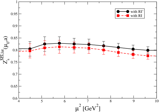
In Fig. 13, we plot our result $\mathcal{Z}^{\overline{\mathrm{MS}},\mathrm{lat}}_{\mathrm{s}}(\mu_{0},a)$ at $\mu_{0}=2\,\mathrm{GeV}$ vs. the matching scale $\mu$ for the intermediate schemes $\mathrm{RI}$ and $\mathrm{RI}^{\prime}$ . If the non-perturbative, cut-off and higher order perturbative effects were negligible, the two curves would coincide and would be independent of the choice of $\mu$ . Taking the average values for $2\,\mathrm{GeV}\leq\mu\leq 3\,\mathrm{GeV}$ and taking into account the slight difference between the curves, we get

\mathcal{Z}^{\overline{\mathrm{MS}},\mathrm{lat}}_{\mathrm{s}}(\mu_{0}=2\,\mathrm{GeV},a)=0.82(3)

(A-6)

References

[1] S. Weinberg, Physica A96 (1979) 327.
[2] J. Gasser and H. Leutwyler, Phys. Lett. B 125 (1983) 321, 325.
[3] J. Gasser and H. Leutwyler, Ann. Phys. (N.Y.). 158 (1984) 142.
[4] J. Gasser and H. Leutwyler, Nucl. Phys. B 250 (1985) 465.
[5] J. Gasser and H. Leutwyler, Phys. Lett. B 184 (1987) 83; 188 (1987) 477.
[6] J. Gasser and H. Leutwyler, Nucl. Phys. B 307 (1988) 763.
[7] P. Hasenfratz and H. Leutwyler, Nucl. Phys. B 343 (1990) 241.
[8] F. C. Hansen, Nucl. Phys. B 345 (1990) 685.
[9] E. V. Shuryak and J. J. M. Verbaarschot, Nucl. Phys. A 560 (1993) 306 [arXiv:hep-th/9212088],
J. J. M. Verbaarschot and T. Wettig, Ann. Rev. Nucl. Part. Sci 50 (2000) 343 [arXiv:hep-ph/0003017],
P. H. Damgaard and S. M. Nishigaki, Phys. Rev. 63 (2001) 045012 [arXiv:hep-th/0006111]
[10] R. G. Edwards, U. M. Heller, J. E. Kiskis and R. Narayanan, Phys. Rev. Lett. 82 (1999) 4188.
[11] W. Bietenholz, K. Jansen and S. Shcheredin, JHEP 0307 (2003) 033.
[12] W. Bietenholz, Th. Chiarappa, K. Jansen Kei-ichi Nagai and S. Shcheredin, JHEP 0402 (2004) 023.
[13] L. Giusti, M. Lüscher, P. Weisz and H. Wittig, JHEP 0311 (2003) 23 [arXiv:hep-lat/0309189].
[14] L. Giusti, P. Hernandez, M. Laine, P. Weisz and H. Wittig, JHEP 0404 (2004) 013 [arXiv:hep-lat/0402002].
[15] R. G. Edwards, Nucl. Phys. Proc. Suppl. 106 (2002) 38 [arXiv:hep-lat/0111009].
[16] T. DeGrand and S. Schaefer, Comput. Phys. Commun. 159 (2004) 185 [arXiv:hep-lat/0401011].
[17] L. Giusti, C. Hoelbling, M. Lüscher and H. Wittig, Comput. Phys. Commun. 153 (2003) 31 [arXiv:hep-lat/0212012].
[18] L. Giusti and S. Necco, JHEP 0704 (2007) 090 [arXiv:hep-lat/0702013].
[19] P. H. Damgaard, Nucl. Phys. Proc. Suppl. 128 (2004) 47 [arXiv:hep-lat/0310037].
[20] H. Neuberger, Phys. Lett. B 417 (1998) 141 [arXiv:hep-lat/9707022]; 427 (1998) 353 [arXiv:hep-lat/9801031].
[21] T. DeGrand and S. Schaefer, Phys. Rev. D 71 (2005) 034507 [arXiv:hep-lat/0412005]; 72 (2005) 054503 [arXiv:hep-lat/0506021]; PoS LAT2005 (2006) 140 [arXiv:hep-lat/0508025].
[22] Th. DeGrand, Zh. Liu, S. Schaefer, Phys. Rev. D 74 (2006) 094504, Erratum-ibid. D 74 (2006) 099904 [arXiv:hep-lat/0608019];
[23] H. Fukaya et al. [JLQCD Collaboration], Phys. Rev. Lett. 98, 172001 (2007) [arXiv:hep-lat/0702003].
[24] P. Hasenfratz, S. Hauswirth, K. Holland, T. Jorg, F. Niedermayer and U. Wenger, Int. J. Mod. Phys. C 12 (2001) 691 [arXiv:hep-lat/0003013],
P. Hasenfratz, S. Hauswirth, T. Jorg, F. Niedermayer and K. Holland, Nucl. Phys.B 643 (2002) 280 [arXiv:hep-lat/0205010],
C. Gattringer et al. Bern-Graz-Regensburg Collaboration, Nucl.Phys.B 677 (2004) 3 [arXiv:hep-lat/0307013],
P. Hasenfratz, K. J. Juge and F. Niedermayer, Bern-Graz-Regensburg Collaboration, JHEP 0412:030,2004 [arXiv:hep-lat/0411034].
[25] A. Hasenfratz, P. Hasenfratz and F. Niedermayer, Phys.Rev. D72 (2005) 114508 [arXiv:hep-lat/0506024].
[26] A. Hasenfratz and F. Knechtli, Comput. Phys. Commun. 148 (2002) 81 [arXiv:hep-lat/0203010].
[27] M. Grady, Phys. Rev. D 32 (1985) 1496 [arXiv:hep-lat/0203010].
[28] M. Creutz, Algorithms for Simulating Fermions (1992), in Quantum Fields on the Computer, World Scientific Publishing.
[29] A. Alexandru and A. Hasenfratz, Phys. Rev. D 65 (2002) 114506 [arXiv:hep-lat/0203026]; 66 (2002) 094502 [arXiv:hep-lat/0207014].
[30] F. Knechtli and U. Wolff, (Alpha Coll.) Nucl. Phys. B 663 (2003) 3 [arXiv:hep-lat/0303001].
[31] M. Hasenbusch, Phys. Lett. B 519 (2001) 177 [arXiv:hep-lat/0107019].
[32] P. de Forcrand, Nucl. Phys.proc. Suppl. 119 (1999) [arXiv:hep-lat/9809145].
[33] A. D. Kennedy and J. Kuti, Phys. Rev. Lett. 54 (1985) 2473.
[34] A. D. Kennedy, J. Kuti, S. Meyer and B. J. Pendleton, Phys. Rev. D 38 (1988) 627.
[35] B. Joo, I. Horvath and K, F. Liu, Phys. Rev. D 67 (2003) 074505 [arXiv:hep-lat/0112033].
[36] I. Montvay and E. Scholz, Phys. Lett. B 623 (2005) 73 [arXiv:hep-lat/0506006].
[37] M. Weingart, ’Stochastic Estimator of the $s$ Quark Determinant in Full QCD Simulation’, Diploma work, Uni. Bern, 2007.
[38] R. Sommer, Nucl. Phys. B 411 839 (1994) [arXiv:hep-lat/9310022].
[39] A. Hasenfratz, P. Hasenfratz, D. Hierl, F. Niedermayer and A. Schäfer, PoS LAT2006 (2006) 178 [arXiv:hep-lat/0610096].
[40] P. Hasenfratz,V. Laliena and F. Niedermayer, Phys. Lett. B 427 (1998) 125 [arXiv:hep-lat/9801021].
[41] H. Neuberger, Phys. Rev. Lett, 60 (1988) 880; Nucl. Phys. B 300 [FS22] (1988) 180.
[42] G. Martinelli, C. Pittori, C. T. Sachrajda, M. Testa and A. Vladikas, Nucl. Phys. B 445 (1995) 81 [arXiv:hep-lat/9411010].
[43] V. Maillart and F. Niedermayer, arXiv:0807.0030 [hep-lat].
[44] E. Franco and V. Lubicz, Nucl. Phys. B 531 (1998) 641 [arXiv:hep-ph/9803491].
[45] K. G. Chetyrkin and A. Retey, Nucl. Phys. B 583 (2000) 3 [arXiv:hep-ph/9910332].
[46] K. G. Chetyrkin, Phys. Lett. B 404 (1997) 161 [arXiv:hep-ph/9703278].
[47] J. A. M. Vermaseren, S. A. Larin and T. van Ritbergen, Phys. Lett. B 405 (1997) 327 [arXiv:hep-ph/9703284].
[48] T. van Ritbergen, J. A. M. Vermaseren and S. A. Larin, Phys. Lett. B 400 (1997) 379 [arXiv:hep-ph/9701390].
[49] Y. Aoki et al., Phys. Rev. D 78 (2008) 054510, arXiv:0712.1061 [hep-lat].
[50] W. M. Yao et al. [Particle Data Group], J. Phys. G 33 (2006) 1.