The squeezed generalized amplitude damping channel

Abstract

Squeezing of a thermal bath introduces new features absent in an open quantum system interacting with an uncorrelated (zero squeezing) thermal bath. The resulting dynamics, governed by a Lindblad-type evolution, extends the concept of a generalized amplitude damping channel, which corresponds to a dissipative interaction with a purely thermal bath. Here we present the Kraus representation of this map, which we call the squeezed generalized amplitude damping channel. As an application of this channel to quantum information, we study the classical capacity of this channel.

I Introduction

The concept of open quantum systems is a ubiquitous one in that any real system of interest is surrounded by its environment (reservoir or bath), which influences its dynamics. They provide a natural route for discussing damping and dephasing. One of the first testing grounds for open system ideas was in quantum optics wl73 . Its application to other areas gained momentum from the works of Caldeira and Leggett cl83 , and Zurek wz93 among others. Depending upon the system-reservoir ($S-R$) interaction, open systems can broadly be classified into two categories, viz., quantum non-demolition (QND) or dissipative. A particular type of quantum nondemolition (QND) $S-R$ interaction is given by a class of energy-preserving measurements in which dephasing occurs without damping the system. This may be achieved when the Hamiltonian $H_{S}$ of the system commutes with the Hamiltonian $H_{SR}$ describing the system-reservoir interaction, i.e., $H_{SR}$ is a constant of the motion generated by $H_{S}$ sgc96 ; mp98 ; gkd01 . A dissipative open system would be when $H_{S}$ and $H_{SR}$ do not commute resulting in dephasing along with damping bp02 . A prototype of dissipative open quantum systems, having many applications, is the quantum Brownian motion of harmonic oscillators. This model was studied by Caldeira and Leggett cl83 for the case where the system and its environment were initially separable. The above treatment of the quantum Brownian motion was generalized to the physically reasonable initial condition of a mixed state of the system and its environment by Hakim and Ambegaokar ha85 , Smith and Caldeira sc87 , Grabert, Schramm and Ingold gsi88 , and for the case of a system in a Stern-Gerlach potential sb00 , and also for the quantum Brownian motion with nonlinear system-environment couplings sb03-2 , among others. The interest in the relevance of open system ideas to quantum information and quantum computation has burgeoned in recent times because of the impressive progress made on the experimental front in the manipulation of quantum states of matter towards quantum information processing and quantum communication.

A number of open system effects can be given an operator-sum or Kraus representation kraus . In this representation, a superoperator ${\cal E}$ due to interaction with the environment, acting on the state of the system is given by

$$\rho\longrightarrow{\cal E}(\rho)=\sum_{k}\langle e_{k}|U(\rho\otimes|f_{0}\rangle\langle f_{0}|)U^{{\dagger}}|e_{k}\rangle=\sum_{j}E_{j}\rho E_{j}^{{\dagger}},$$ (1)

where $U$ is the unitary operator representing the free evolution of the system, reservoir, as well as the interaction between the two, $\{|f_{0}\rangle\}$ is the environment’s initial state, and $\{|e_{k}\rangle\}$ is a basis for the environment. The environment and the system are assumed to start in a separable state. The $E_{j}\equiv\langle e_{k}|U|f_{0}\rangle$ are the Kraus operators, which satisfy the completeness condition $\sum_{j}E_{j}^{{\dagger}}E_{j}=\mathcal{I}$. It can be shown that any transformation that can be cast in the form (1) is a completely positive (CP) map nc00 .

To connect the predicted effects to actual experiments, a detailed model of the interaction between the principal system and the environment is required. However, from the viewpoint of a number of applications to quantum computation and information processing, these details may not be of immediate relevance. In such a case, the Kraus representation is useful because it provides an intrinsic description of the principal system, without explicitly considering the detailed properties of the environment nc00 . The essential features of the problem are contained in the operators $E_{k}$. This not only simplifies calculations, but often provides theoretical insight. An example we will encounter below is the interplay between environmental squeezing and thermal effects for the case of dissipative system-reservoir interactions. Moreover, the reduced dynamics of a number of, seemingly different, physical systems could be modelled in the quantum operations formalism nc00 by the same noisy channel. This would help in the development of insight into the common features of the reduced dynamics of the above systems. For example, for the case of a two-level system interacting, via a quantum non-demolition (QND) interaction, either with a bath of two-level systems (in the weak coupling limit) or harmonic oscillators (at zero temperature $T$ and zero bath squeezing), the reduced dynamics in the quatum operations formalism can be shown to be governed by the phase damping channel srigp ; bg06 . Another example would be the reduced dynamics of a simplified Jaynes-Cummings model consisting of a two-level atom coupled to a single cavity mode which in turn is interacting with a vacuum bath of harmonic oscillators. This can, considering only a single excitation in the atom-cavity system, be shown to be generated by an amplitude damping channel. Since as shown below, an amplitude damping channel results generally from the interactions governed by the Lindblad type of evolution (at zero $T$ and zero bath squeezing), this enables us to get an understanding of the reduced dynamics of the above system without having to concern ourselves with particular details.

In this paper we study an open system, taken to be two-level system or qubit, where the bath is taken to be initially in a squeezed thermal state. The resulting dynamics, governed by a Lindblad-type evolution, generates a completely positive map that extends the concept of a generalized amplitude damping channel, which corresponds to a dissipative interaction with a purely thermal bath. We present the Kraus representation of this map, which we call the squeezed generalized amplitude damping channel. An advantage of using a squeezed thermal bath is that the decay rate of quantum coherence can be suppressed leading to preservation of nonclassical effects bg06 ; kw88 ; kb93 . It has also been shown to modify the evolution of the geometric phase of two-level atomic systems srigp . The preservation of entanglement in the presence of a squeezed bath has been investigated in Ref. wlk02 .

The paper is organized as follows. In Section II, we obtain the evolution of a qubit in a dissipative (non-QND) interaction with its bath. In Section II.1, we consider, in specific, a system interacting with a squeezed thermal bath in the weak Born-Markov rotating wave approximation. In Section II.2, we consider a single-mode Jaynes-Cummings model in a vacuum bath. The amplitude damping and generalized amplitude damping channels are introduced in Section III, where it is pointed out that the simplified Jaynes-Cummings model realizes an amplitude damping channel, while the weak Born-Markov interaction without bath squeezing realizes a generalized amplitude damping channel. We introduce the squeezed generalized amplitude damping channel, which extends the concept of generalized amplitude damping noise, to the case where environmental squeezing is included, in Section IV. Of particular interest is the fact that unlike the case of a purely dephasing channel, where the action of squeezing and temperature are concurrently decohering, in the case of squeezed generalized amplitude damping channel, they can exhibit counteractive behavior srigp ; sriph . In specific, in Section V, where we study the classical capacity of a squeezed generalized amplitude damping channel, we show that squeezing can improve the channel capacity, whereas temperature necessarily degrades it. We make our conclusions in Section VI.

II Two-level system in non-QND interaction with bath

In this section we study the dynamics of a two-level system in a dissipative interaction with its bath, which is taken as one composed of harmonic oscillators. We first consider the case of the system interacting with a bath which is initially in a squeezed thermal state, in the weak coupling Born-Markov, rotating wave approximation. Next we consider a simple single mode Jaynes-Cummings model in a vacuum bath.

II.1 System interacting with bath in the weak Born-Markov, rotating-wave approximation

Here we take up the case of a two-level system interacting with a squeezed thermal bath in the weak Born-Markov, rotating wave approximation. The system Hamiltonian is given by $H_{S}=(\hbar\omega/2)\sigma_{z}$. The system interacts with the bath of harmonic oscillators via the atomic dipole operator which in the interaction picture is given as $\vec{D}(t)=\vec{d}\sigma_{-}e^{-i\omega t}+\vec{d^{*}}\sigma_{+}e^{i\omega t}$ where $\vec{d}$ is the transition matrix elements of the dipole operator. The evolution of the reduced density matrix operator of the system $S$ in the interaction picture has the following form sz97 ; bp02

$${d\over dt}\rho^{s}(t) = \gamma_{0}(N+1)\left(\sigma_{-}\rho^{s}(t)\sigma_{+}-{1\over 2}\sigma_{+}\sigma_{-}\rho^{s}(t)-{1\over 2}\rho^{s}(t)\sigma_{+}\sigma_{-}\right)$$ (2)

$$+ \gamma_{0}N\left(\sigma_{+}\rho^{s}(t)\sigma_{-}-{1\over 2}\sigma_{-}\sigma_{+}\rho^{s}(t)-{1\over 2}\rho^{s}(t)\sigma_{-}\sigma_{+}\right)$$

$$- \gamma_{0}M\sigma_{+}\rho^{s}(t)\sigma_{+}-\gamma_{0}M^{*}\sigma_{-}\rho^{s}(t)\sigma_{-}.$$

Here $\gamma_{0}$ is the spontaneous emission rate given by $\gamma_{0}=(4\omega^{3}|\vec{d}|^{2})/(3\hbar c^{3})$, and $\sigma_{+}$, $\sigma_{-}$ are the standard raising and lowering operators, respectively given by $\sigma_{+}=|1\rangle\langle 0|=\frac{1}{2}\left(\sigma_{x}+i\sigma_{y}\right)$ and $\sigma_{-}=|0\rangle\langle 1|={1\over 2}\left(\sigma_{x}-i\sigma_{y}\right)$. Eq. (2) may be expressed in a manifestly Lindblad form as srigp

$$\frac{d}{dt}\rho^{s}(t)=\sum_{j=1}^{2}\left(2R_{j}\rho^{s}R^{{\dagger}}_{j}-R_{j}^{{\dagger}}R_{j}\rho^{s}-\rho^{s}R_{j}^{{\dagger}}R_{j}\right),$$ (3)

where $R_{1}=(\gamma_{0}(N_{\rm th}+1)/2)^{1/2}R$, $R_{2}=(\gamma_{0}N_{\rm th}/2)^{1/2}R^{{\dagger}}$ and $R=\sigma_{-}\cosh(r)+e^{i\Phi}\sigma_{+}\sinh(r)$. This observation guarantees that the evolution of the density operator can be given a Kraus or operator-sum representation nc00 , a point we return to in Section IV. If $T=0$, then $R_{2}$ vanishes, and a single Lindblad operator suffices to describe Eq. (2).

A number of methods of generating bath squeezing have been proposed in the literature. A squeezed reservoir may be constructed on the basis of establishment of squeezed light field buz91 . A single-mode squeezed state created in a degenerate parametric amplifier operated in an appropriate cavity, when coupled to an infinite number of external “output” modes, transfers the squeezing into correlations between side-bands of the multimode light field. A subthreshold optical parametric oscillator (OPO) can be used as the basis for the implementation of a stable, reliable source of continuous-wave squeezed vacuum bre95 . Experiments probing the squeezed-light-atom system have been carried out in Refs. geo95 ; tur98 . In particular, the latter reference details a method in which an OPO operated below threshold downconverts a high energy photon into two correlated low energy photons generating a close-to-minimum-uncertainty squeezed vacuum state. At the output of the OPO, the squeezed vacuum is mixed on a 99-1 beam-splitter with a phase-coherent reference oscillator with controlled relative phase to the squeezing, resulting in a combined electromagnetic field that is equivalent to a displaced squeezed state.

An infinite array of beam-splitters can be used to model a squeezed reservoir kim95 . The signal is injected from the left of the array, with independent squeezed fields (all with the same properties) injected into the other ports. The output of a given beam-splitter serves as input to the subsequent one. In the limit of an infinite number of beam-splitters, the dynamics generated by Eq. (2) is simulated. In Ref. poy96 , quantum reservoir engineering with laser-cooled trapped ions is used to mimic the dynamics of an atom interacting with a squeezed vacuum bath (Eq. (2) with temperature $T$ set to zero). Another way to engineer a quantum reservoir to mimic coupling with a squeezed bath has been proposed in Ref. lut98 . They consider a four-level system with two (degenerate) ground and excited states, driven by weak laser fields and coupled to a vacuum reservoir of radiation modes. Interference between the spontaneous emission channels in optical pumping leads to a squeezed bath type coupling for the two-level system constituted by the two ground levels. The properties of the squeezed bath are shown to be controllable by means of the laser parameters. An experimental study of the decoherence and decay of quantum states of a trapped atomic ion’s harmonic motion with several types of engineered reservoirs, including amplitude dampling and generalized amplitude damping channels, have been made in Refs. mya00 ; tur00 .

In Eqs. (2) and (3), we use the nomenclature $|1\rangle$ for the upper state and $|0\rangle$ for the lower state and $\sigma_{x},\sigma_{y},\sigma_{z}$ are the standard Pauli matrices. In Eq. (2),

$$N=N_{\rm th}(\cosh^{2}(r)+\sinh^{2}(r))+\sinh^{2}(r),$$ (4)

and $M=-\frac{1}{2}\sinh(2r)e^{i\Phi}(2N_{\rm th}+1)$, and $N_{\rm th}=1/(e^{\hbar\omega/k_{B}T}-1)$. Here $N_{\rm th}$ is the Planck distribution giving the number of thermal photons at the frequency $\omega$ and $r$, $\Phi$ are bath squeezing parameters cs85 . The analogous case of a thermal bath without squeezing can be obtained from the above expressions by setting these squeezing parameters to zero. We solve the Eq. (2) using the Bloch vector formalism as

$$\rho^{s}(t)={1\over 2}\left(\mathcal{I}+\langle\vec{\sigma}(t)\rangle\cdot\vec{\sigma}\right)=\begin{pmatrix}{1\over 2}\left(1+\langle\sigma_{z}(t)\rangle\right)&\langle\sigma_{-}(t)\rangle\cr\langle\sigma_{+}(t)\rangle&{1\over 2}\left(1-\langle\sigma_{z}(t)\rangle\right)\end{pmatrix}.$$ (5)

In Eq. (5) by the vector $\vec{\sigma}(t)$ we mean $(\sigma_{x}(t),\sigma_{y}(t),\sigma_{z}(t))$ and $\langle\vec{\sigma}(t)\rangle$ denotes the Bloch vectors which are solved using Eq. (2) to yield srigp

$$\langle\sigma_{x}(t)\rangle = \left[1+{1\over 2}\left(e^{\gamma_{0}at}-1\right)(1+\cos(\Phi))\right]e^{-{\gamma_{0}\over 2}(2N+1+a)t}\langle\sigma_{x}(0)\rangle-\sin(\Phi)\sinh({\gamma_{0}at\over 2})e^{-{\gamma_{0}\over 2}(2N+1)t}\langle\sigma_{y}(0)\rangle,$$

$$\langle\sigma_{y}(t)\rangle = \left[1+{1\over 2}\left(e^{\gamma_{0}at}-1\right)(1-\cos(\Phi))\right]e^{-{\gamma_{0}\over 2}(2N+1+a)t}\langle\sigma_{y}(0)\rangle-\sin(\Phi)\sinh({\gamma_{0}at\over 2})e^{-{\gamma_{0}\over 2}(2N+1)t}\langle\sigma_{x}(0)\rangle,$$

$$\langle\sigma_{z}(t)\rangle = e^{-\gamma_{0}(2N+1)t}\langle\sigma_{z}(0)\rangle-{1\over(2N+1)}\left(1-e^{-\gamma_{0}(2N+1)t}\right).$$ (6)

In these equations $a=\sinh(2r)(2N_{th}+1)$. Using the Eqs. (II.1) in Eq. (5) and then reverting back to the Schrödinger picture, the reduced density matrix of the system can be written as

$$\rho^{s}(t)=\begin{pmatrix}{1\over 2}(1+A)&Be^{-i\omega t}\cr B^{*}e^{i\omega t}&{1\over 2}(1-A)\end{pmatrix},$$ (7)

where, in view of Eq. (5),

$$A\equiv\langle\sigma_{z}(t)\rangle=e^{-\gamma_{0}(2N+1)t}\langle\sigma_{z}(0)\rangle-{1\over(2N+1)}\left(1-e^{-\gamma_{0}(2N+1)t}\right),$$ (8)

$$B=\left[1+{1\over 2}\left(e^{\gamma_{0}at}-1\right)\right]e^{-{\gamma_{0}\over 2}(2N+1+a)t}\langle\sigma_{-}(0)\rangle+\sinh({\gamma_{0}at\over 2})e^{i\Phi-{\gamma_{0}\over 2}(2N+1)t}\langle\sigma_{+}(0)\rangle.$$ (9)

From Eq. (II.1), it is seen that the system evolves towards a fixed asymptotic point in the Bloch sphere bg06 , which in general is not a pure state, but the mixture

$$\rho_{\rm asymp}=\left(\begin{array}[]{ll}1-q&0\\ 0&q\end{array}\right),$$ (10)

where $q=\frac{N+1}{2N+1}$. If $T=0$ and $r=0$, then $q=1$, and the pure state $|0\rangle$ is reached asymptotically, an observation that serves as the basis for the quantum deleter qdele .

II.2 Simplified Jaynes-Cummings Model

Here we consider a simplified Jaynes-Cummings model taking into account the effect of the environment, which is modelled as a zero temperature bath. In this model we consider the case of only a single excitation in the atom-cavity system with the bath modelling the effect of imperfect cavity mirrors. Also the cavity frequency is assumed to be in resonance with the atomic frequency bp02 ; bg97 . The total Hamiltonian is

$$H=H_{S}+H_{R}+H_{SR}=\omega_{0}\sigma_{+}\sigma_{-}+\sum\limits_{k}\omega_{k}b^{\dagger}_{k}b_{k}+\sigma_{+}\sum\limits_{k}g_{k}b_{k}+\sigma_{-}\sum\limits_{k}g^{*}_{k}b^{\dagger}_{k}.$$ (11)

Here $H_{S}$, $H_{R}$ and $H_{SR}$ stand for the Hamiltonians of the system, reservoir and system reservoir interaction, respectively. In the case of a single excitation in the atom-cavity system, the cavity mode can be eliminated in favour of the following effective spectral density

$$I(\omega)={1\over 2\pi}{\gamma_{0}\kappa^{2}\over(\omega_{0}-\omega)^{2}+\kappa^{2}}.$$ (12)

Here $\omega_{0}$ is the atomic transition frequency and $\kappa$ is the spectral width of the system-environment coupling. Tracing over the vacuum bath and assuming that initially there are no photons, the reduced density matrix of the atom (two-level system) can be obtained in the Schrödinger representation as

$$\rho^{s}(t)=\begin{pmatrix}a&be^{-i\omega_{0}t}\cr b^{*}e^{i\omega_{0}t}&(1-a)\end{pmatrix},$$ (13)

where

$$a = \rho_{{1\over 2},{1\over 2}}(0)e^{-\kappa t}\left[\cosh\left({lt\over 2}\right)+{\kappa\over l}\sinh\left({lt\over 2}\right)\right]^{2},$$ (14a)

$$b = \rho_{{1\over 2},-{1\over 2}}(0)e^{-{\kappa t\over 2}}\left[\cosh\left({lt\over 2}\right)+{\kappa\over l}\sinh\left({lt\over 2}\right)\right].$$ (14b)

Here $l=\sqrt{\kappa^{2}-2\gamma_{0}\kappa}$, where $\gamma_{0},\kappa$ are as in Eq. (12). Initially the system is chosen to be in the state

$$|\psi(0)\rangle=\cos({\theta_{0}\over 2})|1\rangle+e^{i\phi_{0}}\sin({\theta_{0}\over 2})|0\rangle.$$ (15)

From the above equation, it can be easily seen that $\rho_{{1\over 2},{1\over 2}}(0)=\cos^{2}({\theta_{0}\over 2})$ and $\rho_{{1\over 2},-{1\over 2}}(0)={1\over 2}e^{-i\phi_{0}}\sin(\theta_{0})$.

III Amplitude damping and Generalized Amplitude damping channels

The generalized amplitude channel is generated by the evolution given by the master equation (2), with the bath squeezing parameters $r$ and $\Phi$ set to zero. Generalized amplitude damping channels capture the idea of energy dissipation from a system, for example, in the spontaneous emission of a photon, or when a spin system at high temperature approaches equilibrium with its environment (also cf. Refs. mya00 ; tur00 ). A simple model of an amplitude damping channel is the scattering of a photon via a beam-splitter. One of the output modes is the environment, which is traced out. The unitary transformation at the beam-splitter is given by $B=\exp\left[\theta(a^{{\dagger}}b-ab^{{\dagger}})\right]$, where $a,b$ and $a^{{\dagger}},b^{{\dagger}}$ are the annihilation and creation operators for photons in the two modes.

III.1 Amplitude damping channel

This channel is generated by the evolution given by the master equation (2), with temperature $T$ and bath squeezing parameters $r$ and $\Phi$ set to zero. The corresponding Kraus operators are:

$$\begin{array}[]{ll}E_{0}\equiv\left[\begin{array}[]{ll}\sqrt{1-\lambda(t)}&0\\ 0&1\end{array}\right];{}{}{}{}&E_{1}\equiv\left[\begin{array}[]{ll}0&0\\ \sqrt{\lambda(t)}&0\end{array}\right].\end{array}$$ (21)

The effect of these operators is to produce the completely positive map

$$\sum_{j}E_{j}\left(\begin{array}[]{ll}A&B^{*}\\ B&1-A\end{array}\right)E^{{\dagger}}_{j}=\left(\begin{array}[]{ll}A(1-\lambda)&\sqrt{1-\lambda}B^{*}\\ \sqrt{1-\lambda}B&1-A+\lambda A\end{array}\right),$$ (22)

where, on comparison with Eq. (15), we see that $A=\cos^{2}(\theta_{0}/2)$, $B=(1/2)e^{i\phi_{0}}\sin(\theta_{0})$. The simplified Jaynes-Cummings model of the previous subsection is easily seen to realize an amplitude damping channel. It is straightforward to verify that with the identification

$$1-\lambda(t)\equiv e^{-{\kappa t}}\left[\cosh\left({lt\over 2}\right)+{\kappa\over l}\sinh\left({lt\over 2}\right)\right]^{2}.$$ (23)

the operators (21), acting on the state (15), reproduce the evolution (13) (in the interaction picture).

III.2 Generalized amplitude damping channel

This channel is generated by the evolution governed by the master equation (2), with bath squeezing parameters $r$ and $\Phi$ set to zero, but $T$ not necessarily zero. The corresponding Kraus operators are:

$$\begin{array}[]{ll}E_{0}\equiv\sqrt{p}\left[\begin{array}[]{ll}\sqrt{1-\lambda(t)}&0\\ 0&1\end{array}\right];{}{}{}{}&E_{1}\equiv\sqrt{p}\left[\begin{array}[]{ll}0&0\\ \sqrt{\lambda(t)}&0\end{array}\right];\\ E_{2}\equiv\sqrt{1-p}\left[\begin{array}[]{ll}1&0\\ 0&\sqrt{1-\lambda(t)}\end{array}\right];{}{}{}{}&E_{3}\equiv\sqrt{1-p}\left[\begin{array}[]{ll}0&\sqrt{\lambda(t)}\\ 0&0\end{array}\right],\end{array}$$ (34)

where $0\leq p\leq 1$ nc00 ; srigp .

The effect of these operators is to produce the completely positive map

$$\sum_{j}E_{j}\left(\begin{array}[]{ll}A&B^{*}\\ B&1-A\end{array}\right)E^{{\dagger}}_{j} = p\left(\begin{array}[]{ll}A(1-\lambda)&\sqrt{1-\lambda}B^{*}\\ \sqrt{1-\lambda}B&1-A+\lambda A\end{array}\right)$$ (42)

$$+(1-p)\left(\begin{array}[]{ll}A+\lambda(1-A)&\sqrt{1-\lambda}B^{*}\\ \sqrt{1-\lambda}B&1-A+(1-\lambda)(1-A)\end{array}\right).$$

It is straightforward to verify that with the identification

$$\lambda(t)\equiv 1-e^{-\gamma_{0}(2N_{\rm th}+1)t};\hskip 28.45274ptp\equiv\frac{N_{\rm th}+1}{2N_{\rm th}+1},$$ (43)

the operators (34) acting on the state (15) reproduce the evolution (II.1), with squeezing set to zero but temperature non-vanishing, by means of the map given by Eq. (1). If $T=0$, then $p=1$, reducing Eq. (34) to the amplitude damping channel, given by Eq. (21).

IV The squeezed generalized amplitude damping channel

This channel is generated by the evolution given by the master equation (2), with neither the bath squeezing parameters $r$ and $\Phi$ nor the temperature $T$ necessarily zero. Thus this is a very general (completely positive) map generated by Eq. (2). To generalize (34) to include the effects of squeezing, we construct the following set of Kraus operators:

$$\begin{array}[]{ll}E_{0}\equiv\sqrt{p_{1}}\left[\begin{array}[]{ll}\sqrt{1-\alpha(t)}&0\\ 0&\sqrt{1-\beta(t)}\end{array}\right];{}{}{}{}&E_{1}\equiv\sqrt{p_{1}}\left[\begin{array}[]{ll}0&\sqrt{\beta(t)}\\ \sqrt{\alpha(t)}e^{-i\phi(t)}&0\end{array}\right];\\ E_{2}\equiv\sqrt{p_{2}}\left[\begin{array}[]{ll}\sqrt{1-\mu(t)}&0\\ 0&\sqrt{1-\nu(t)}\end{array}\right];{}{}{}{}&E_{3}\equiv\sqrt{p_{2}}\left[\begin{array}[]{ll}0&\sqrt{\nu(t)}\\ \sqrt{\mu(t)}e^{-i\theta(t)}&0\end{array}\right].\\ \end{array}$$ (54)

It is readily checked that Eq. (54) satisfies the completeness condition

$$\sum_{j=0}^{3}E_{j}^{{\dagger}}E_{j}=\mathbb{I},$$ (55)

provided

$$p_{1}+p_{2}=1.$$ (56)

Substituting the Kraus operator elements given by Eq. (54) in Eq. (1), and using Eq. (5), yields the following Bloch vector evolution equations:

$$\langle\sigma_{x}(t)\rangle = \left[(p_{1}\sqrt{(1-\alpha(t))(1-\beta(t))})+p_{2}\sqrt{(1-\mu(t))(1-\nu(t))}+(p_{1}\sqrt{\alpha(t)\beta(t)}\cos\phi+p_{2}\sqrt{\mu(t)\nu(t)}\cos\theta)\right]\langle\sigma_{x}(0)\rangle$$ (57a)

$$- \left[(p_{1}\sqrt{\alpha(t)\beta(t)}\sin\phi+p_{2}\sqrt{\mu(t)\nu(t)}\sin\theta)\right]\langle\sigma_{y}(0)\rangle,$$

$$\langle\sigma_{y}(t)\rangle = \left[(p_{1}\sqrt{(1-\alpha(t))(1-\beta(t))}+p_{2}\sqrt{(1-\mu(t))(1-\nu(t))})-(p_{1}\sqrt{\alpha(t)\beta(t)}\cos\phi+p_{2}\sqrt{\mu(t)\nu(t)}\cos\theta)\right]\langle\sigma_{y}(0)\rangle$$ (57b)

$$- \left[(p_{1}\sqrt{\alpha(t)\beta(t)}\sin\phi+p_{2}\sqrt{\mu(t)\nu(t)}\sin\theta)\right]\langle\sigma_{x}(0)\rangle,$$

$$\langle\sigma_{z}(t)\rangle = (1-p_{2}(\mu(t)+\nu(t))-p_{1}(\alpha(t)+\beta(t)))\langle\sigma_{z}(0)\rangle-p_{2}(\mu(t)-\nu(t))-p_{1}(\alpha(t)-\beta(t)).$$ (57c)

Comparing Eqs. (57) with Eqs. (II.1), we can read off the corresponding terms. In fact, the system is underdetermined as there are more variables than constraints. An inspection of Eqs. (II.1) shows that they yield a total of 5 constraints on the channel variables, $p_{1}$, $p_{2}$, $\mu$, $\nu$, $\alpha$, $\beta$, $\theta$ and $\phi$, with a further constraint coming from Eq. (56). The two redundant variables may be conveniently chosen to be $\beta$ and $\phi$. Setting $\beta=\phi=0$, a comparison of Eqs. (57) and (II.1) produces the following relations:

$$p_{1}\sqrt{(1-\alpha(t))}+p_{2}\sqrt{(1-\mu(t))(1-\nu(t))} = \cosh\left(\frac{\gamma_{0}at}{2}\right)\exp\left(-\frac{\gamma_{0}}{2}(2N+1)t\right),$$ (58a)

$$p_{2}\sqrt{\mu(t)\nu(t)}\cos\theta = \cos(\Phi)\sinh\left(\frac{\gamma_{0}at}{2}\right)\exp\left(-\frac{\gamma_{0}}{2}(2N+1)t\right),$$ (58b)

$$p_{2}\sqrt{\mu(t)\nu(t)}\sin\theta = \sin(\Phi)\sinh\left(\frac{\gamma_{0}at}{2}\right)\exp\left(-\frac{\gamma_{0}}{2}(2N+1)t\right),$$ (58c)

$$p_{1}\alpha(t)+p_{2}(\mu(t)-\nu(t)) = \frac{1}{(2N+1)}\left(1-e^{-\gamma_{0}(2N+1)t}\right),$$ (58d)

$$1-p_{1}\alpha(t)-p_{2}(\mu(t)+\nu(t)) = e^{-\gamma_{0}(2N+1)t},$$ (58e)

and the required squeezed generalized amplitude damping channel is given, in place of Eq. (54), by the Kraus operators

$$\begin{array}[]{ll}E_{0}\equiv\sqrt{p_{1}}\left[\begin{array}[]{ll}\sqrt{1-\alpha(t)}&0\\ 0&1\end{array}\right];{}{}{}{}&E_{1}\equiv\sqrt{p_{1}}\left[\begin{array}[]{ll}0&0\\ \sqrt{\alpha(t)}&0\end{array}\right];\\ E_{2}\equiv\sqrt{p_{2}}\left[\begin{array}[]{ll}\sqrt{1-\mu(t)}&0\\ 0&\sqrt{1-\nu(t)}\end{array}\right];{}{}{}{}&E_{3}\equiv\sqrt{p_{2}}\left[\begin{array}[]{ll}0&\sqrt{\nu(t)}\\ \sqrt{\mu(t)}e^{-i\theta(t)}&0\end{array}\right].\end{array}$$ (69)

It is seen from Eqs. (58) that at time $t=0$, $\mu(0)=\nu(0)=\alpha(0)=0$. We now determine the remaining channel parameters. From Eqs. (58b) and (58c), we find

$$\tan\theta=\tan\Phi,$$ (70)

allowing us to set $\theta=\Phi$, and to identify the channel parameter $\theta$ with the bath squeezing angle. The remaining channel parameters may be identified as follows.

From Eqs. (58d) and (58e), we find

$$\nu(t)=\frac{N}{p_{2}(2N+1)}(1-e^{-\gamma_{0}(2N+1)t}).$$ (71)

Substituting Eq. (71) into Eq. (58c), we find

$$\mu(t)=\frac{2N+1}{2p_{2}N}\frac{\sinh^{2}(\gamma_{0}at/2)}{\sinh(\gamma_{0}(2N+1)t/2)}\exp\left(-\frac{\gamma_{0}}{2}(2N+1)t\right).$$ (72)

Using Eqs. (71) and (72) in (58e), we obtain

$$\alpha(t)=\frac{1}{p_{1}}\left(1-p_{2}[\mu(t)+\nu(t)]-e^{-\gamma_{0}(2N+1)t}\right),$$ (73)

where $\nu(t)$ and $\mu(t)$ are given by Eqs. (71) and (72), respectively.

Substituting Eqs. (71), (72), (73) and (56) into Eq. (58a), we obtain after some manipulations

$$p_{2}(t) = \frac{1}{(A+B-C-1)^{2}-4D}\times\left[A^{2}B+C^{2}+A(B^{2}-C-B(1+C)-D)-(1+B)D-C(B+D-1)\right.$$ (74)

$$\pm \left.2\sqrt{D(B-AB+(A-1)C+D)(A-AB+(B-1)C+D)}\right],$$

where

$$A = \frac{2N+1}{2N}\frac{\sinh^{2}(\gamma_{0}at/2)}{\sinh(\gamma_{0}(2N+1)t/2)}\exp\left(-\gamma_{0}(2N+1)t/2\right),$$

$$B = \frac{N}{2N+1}(1-\exp(-\gamma_{0}(2N+1)t)),$$

$$C = A+B+\exp(-\gamma_{0}(2N+1)t),$$

$$D = \cosh^{2}(\gamma_{0}at/2)\exp(-\gamma_{0}(2N+1)t).$$ (75)

If the squeezing parameter $r$ is set to zero, then $a=0$, and it follows from Eq. (74) and (75), that $\hat{p}_{2}=N_{\rm th}/(2N_{\rm th}+1)$, where the hat indicates that squeezing has been set to zero. It can be seen from Eq. (72), that for zero squeezing ($a=0$), $\hat{\mu}(t)=0$. Substituting $\hat{p}_{2}=N_{\rm th}/(2N_{\rm th}+1)$ in Eq. (71), we find $\hat{\nu}(t)=1-e^{-\gamma_{0}(2N_{\rm th}+1)t}$. Now, a comparison of Eqs. (69) with Eqs. (34) shows that $\hat{\nu}(t)=\lambda(t)$, given by Eq. (43).

Further, in view of Eq. (56), $\hat{p}_{1}=(N_{\rm th}+1)/(2N_{\rm th}+1)$. Substituting Eq. (71) and the conditions $a=0$ and $\hat{\mu}(t)=0$ into Eq. (73), it is easily verified that

$$\hat{\alpha}(t) = \frac{1}{p_{1}}\left(1-p_{2}[\hat{\mu}(t)+\hat{\nu}(t)]-e^{-\gamma_{0}(2N_{\rm th}+1)t}\right)$$ (76)

$$= \frac{2N_{\rm th}+1}{N_{\rm th}+1}\left(\hat{\nu}(t)-\frac{N_{\rm th}}{2N_{\rm th}+1}\hat{\nu}(t)\right)$$

$$= \frac{2N_{\rm th}+1}{N_{\rm th}+1}\left(\frac{N_{\rm th}+1}{2N_{\rm th}+1}\right)\hat{\nu}(t)$$

$$= \hat{\nu}(t).$$

We thus have $\hat{\alpha}(t)=\hat{\nu}(t)=\lambda(t)$, and hence the generalized amplitude damping channel (34) is recovered from Eq. (69) in the limit of vanishing squeezing.

Figure 1: $\nu(t)$ [Eq. (71)] with respect to $t$, with $\gamma_{0}=0.05$. Asymptotically, $\nu(t)$ reaches the value 1. The solid and small-dashed curves corresponds to the temperature (in units where $\hbar\equiv k_{B}\equiv 1$) $T=1$, with the bath squeezing parameter $r=$ 0, 1, respectively, while the large-dashed curve corresponds to $T=3$ and $r=1$.

Figure 1 is a representative plot, showing that for large bath exposure time, $\nu(t)$ approaches 1. This Figure also brings out the concurrent behaviour of temperature and squeezing with respect to $\nu(t)$. At large $t$, $\alpha(t)$ also approaches unity. However, unlike the case of $\nu(t)$, temperature and squeezing can have a contrastive effect on $\alpha(t)$, as brought out in Fig. 2. This contrastive effect of squeezing with respect to time has been observed in the case of mixed state geometric phase srigp and quantum phase diffusion sriph . The dot-dashed curve in Fig. 2 represents a squeezed amplitude damping channel, i.e., a channel given by zero temperature but finite squeezing.

Figure 2: $\alpha(t)$ [Eq. (73)] with respect to time $t$, with $\gamma_{0}=0.05$, bringing out the counteractive effect of squeezing on temperature. Asymptotically, $\alpha(t)$ reaches 1. We find that increasing squeezing reduces $\alpha$ at any fixed temperature, and thus counteracts the thermal effects. The solid and dot-dashed curves correspond to temperature (in units where $\hbar\equiv k_{B}\equiv 1$) $T=0$, with environment squeezing parameter $r=0$ and $1$, respectively. The small-dashed and large-dashed curves correspond to temperature $T=5$, with $r=0$ and 1, respectively.

The fact that as time progresses, squeezing effects tend to die out, leaving thermal effects alone to govern the system evolution, is illustrated in Fig. 3. Squeezing of the bath modes introduces non-stationary effects due to correlations between the modes. This Figure also shows the washing out of these effects with time being accentuated with increase in temperature.

Figure 3: $\mu(t)$ [Eq. (72)] as a function of time $t$, with $\gamma_{0}=0.05$ and $r=1$. The asymptotic value of $\mu(t)$ is 0. The solid, large-dashed and small-dashed curves correspond to temperature (in units where $\hbar\equiv k_{B}\equiv 1$) $T$ equals 20, 5 and 1, respectively.

Figure 4: Probability $p_{2}$ [Eq. (74)] as a function of time $t$ approaches the asymptotic value of $N/(2N+1)$. Here $\gamma_{0}=0.05$. The solid curve corresponds to temperature (in units where $\hbar\equiv k_{B}\equiv 1$) $T=0$ and $r=0.05$. The small-dashed and large-dashed curves correspond to $T=2$, with $r$ equal to 0.1 and 0.5, respectively. We note that the solid line depicts the transformation of the squeezed amplitude damping channel to the amplitude damping channel.

Unlike the case of the generalized amplitude damping channel, here the probabilities $p_{1}(t)$ and $p_{2}(t)$ are time-dependent on account of the presence of non-stationary effects introduced by the bath squeezing (Fig. 4), and $p_{2}(t)$ eventually reaches a stationary value of $N/(2N+1)$, as may be inferred from Eqs. (74) and (75). Substituting this asymptotic value in Eqs. (71), (72) and (73), we find $\nu(\infty)=1$, $\mu(\infty)=0$ and $\alpha(\infty)=1$, as was seen in Figs. 1, 3 and 2, respectively.

In the absence of squeezing, $p_{2}(\infty)$ becomes $N_{\rm th}/(2N_{\rm th}+1)$, consistent with the expression for $p$ in Eq. (43) for the generalized amplitude damping channel. The solid line in Fig. 4 corresponds to the squeezed amplitude damping channel, which for the case of zero bath squeezing yields the action of a quantum deleter qdele via the amplitude damping channel.

If we have $a=0$ and $T=0$, then $\mu(t|a=T=0)=0$, as seen from Eq. (72), and $p_{2}(t)=0$ because $p_{2}(t)$ in Eq. (74) reduces to $N_{\rm th}/(2N_{\rm th}+1)$ when squeezing vanishes. Further, $\nu(t|a=T=0)=\lambda(t|T=0)$ by Eq. (76). Substituting these values in Eqs. (69), we obtain the amplitude damping channel. Eqs. (69) thus furnish a complete representation of a squeezed generalized amplitude damping channel.

V Classical capacity of a squeezed generalized amplitude damping channel

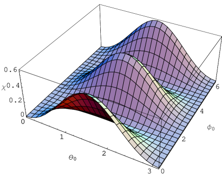
Figure 5: Plotting the Holevo bound $\chi$ [Eq. (77)] for a squeezed amplitude damping channel with $\Phi=0$ and $f=0.5$, over the set $\{\theta_{0},\phi_{0}\}$, which parametrizes the ensemble of input states $\{(\theta_{0},\phi_{0}),~{}(\theta_{0}+\pi,\phi_{0})\}$. Here temperature (in units where $\hbar\equiv k_{B}\equiv 1$) $T=5$, $\gamma_{0}=0.05$, time $t=5.0$ and bath squeezing parameter $r=1$. The channel capacity $C$ is seen to correspond to the optimal value of $\theta_{0}=\pi/2$ [i.e., the input states $\frac{1}{\sqrt{2}}(|0\rangle\pm|1\rangle)$ for $\phi_{0}=0$].

A quantum communication channel can be used to perform a number of tasks, including transmitting classical or quantum information, as well as for the cryptographic purpose of creating shared information between a sender and receiver, that is reliably secret from a malevolent eavesdropper sw98 . A natural question is as to how information communicated over a squeezed generalized amplitude damping channel (denoted ${\cal E})$, and given in the Kraus representation by Eq. (69), is degraded. In this Section, we briefly consider the communication of classical information across the channel sw97 . The problem can be stated as the following game between sender Alice and receiver Bob: Alice has a classical information source producing symbols $X=0,\cdots,n$ with probabilities $p_{0},\cdots,p_{n}$. She encodes the symbols as quantum states $\rho_{j}$ ($0\leq j\leq n$) and communicates them to Bob, whose optimal measurement strategy maximizes his accessible information, which is bounded above by the Holevo quantity

$$\chi=S(\rho)-\sum_{j}p_{j}S(\rho_{j}),$$ (77)

where $\rho=\sum_{j}p_{j}\rho_{j}$, and $\rho_{j}$ are various initial states holevo . In the present case, we assume Alice encodes her binary symbols of 0 and 1 in terms of pure, orthogonal states of the form (15), and transmits them over the squeezed generalized amplitude damping channel.

We further assume that Alice transmits her messages as product states, i.e., without entangling them across multiple channel use. Then, the (product state) classical capacity $C$ of the quantum channel is defined as the maximum of $\chi({\cal E})$ over all ensembles $\{p_{j},\rho_{j}\}$ of possible input states $\rho_{j}$ hau96 ; sww96 . In Fig. 5, we plot $\chi({\cal E})$ over pairs of orthogonal input states $(\theta_{0},\phi_{0})$ and $(\theta_{0}+\pi,\phi_{0})\}$, which correspond to the symbols 0 and 1, respectively, with probability of the input symbol 0 being $f=0.5$. Here we take $\Phi=0$, and the optimum coding is seen to correspond to the choice $(\theta_{0}=\pi/2,\phi_{0}=n\pi)$, where $n\in I$, i.e., the input states $\frac{1}{\sqrt{2}}(|0\rangle\pm|1\rangle)$ or $\frac{1}{\sqrt{2}}(|0\rangle\mp|1\rangle)$.

Fig. 6 depicts $\chi({\cal E})$ for various channel parameters, with the pair of orthogonal input states given by $(\theta_{0},\phi_{0}=0)$ and $(\theta_{0}+\pi,\phi_{0}=0)$. As expected, longer exposure to the channel, or higher temperature, degrades information more, but the optimal choice of input states remains the same as before. Interestingly, squeezing improves the accessible information for input states in a certain range of $\theta_{0}$, but impairs it in other. This is consistent with the understanding that the benefits of squeezing are quadrature-dependent. Fig. 7 demonstrates the contrastive effects of temperature and squeezing on $C$. Comparing the solid and small-dashed curves, one notes that thermal effects tend to degrade $C$, whereas bath squeezing can improve it, as seen by comparing the small- and large-dashed curves. In fact, the improvement due to squeezing is brought out dramatically by a comparison of the solid and large-dashed curves. This highlights the possible usefulness of squeezing to noisy quantum communication.

Figure 6: Optimal source coding for the squeezed amplitude damping channel, with $\chi$ plotted against $\theta_{0}$ corresponding to the “0” symbol. Here $\Phi=0$, $\gamma_{0}=0.05$ and $f=0.5$. It is seen that $\chi$ is maximized for states of the form (15) when the pair of input states are given by $(\theta_{0}=\frac{\pi}{2},\phi_{0}=0)$ and $(\theta_{0}=\frac{\pi}{2}+\pi,\phi_{0}=0)$ [i.e., states $\frac{1}{\sqrt{2}}(|0\rangle\pm|1\rangle)$]. The solid and small-dashed curves represent temperature (in units where $\hbar\equiv k_{B}\equiv 1$) $T=0$ and bath squeezing parameter $r=0$, but $t=1$ and 2, respectively. The large-dashed and dot-dashed curves represent $T=5$ and $t=2$, but with $r=0$ and 2, respectively. A comparison of the solid and small-dashed (small-dashed and large-dashed) curves demonstrates the expected degrading effect on the accessible information, of increasing the bath exposure time $t$ (increasing $T$). A comparison of the large-dashed and dot-dashed curves demonstrates the dramatic effect of including squeezing. In particular, whereas squeezing improves the accessible information for the pair of input states $\frac{1}{\sqrt{2}}(|0\rangle\pm|1\rangle)$, it is detrimental for input states $(\theta_{0},\phi_{0})$ given by $(0,0)$ (i.e., $|1\rangle$) and $(\pi,0)$ (i.e., $|0\rangle$).

Figure 7: Interplay of squeezing and temperature on the classical capacity $C$ of the squeezed amplitude damping channel (with input states $\frac{1}{\sqrt{2}}(|0\rangle\pm|1\rangle)$, and $f=1/2$, corresponding to the optimal coding). Here $\Phi=0$ and $\gamma_{0}=0.05$. The solid and small-dashed curves correspond to zero squeezing $r$, and temperature (in units where $\hbar\equiv k_{B}\equiv 1$) $T=0$ and 5, respectively. The large-dashed curve corresponds to $T=5$ and $r=2$. A comparison between the solid and large-dashed curves shows that squeezing can improve $C$.

VI Conclusions

In this paper we have have obtained a Kraus representation of a noisy channel, which we call the squeezed generalized amplitude damping channel, corresponding to the interaction of a two-level system (qubit) with a squeezed thermal bath via a dissipative interaction. The resulting dynamics, governed by a Lindblad-type evolution, generates a completely positive map that extends the concept of a generalized amplitude damping channel, which corresponds to a dissipative interaction with a purely thermal bath. The physical motivation for studying this channel is that using a squeezed thermal bath the decay rate of quantum coherence can be suppressed, leading to preservation of nonclassical effects. This is in contrast to the case of a purely dephasing channel, where the action of squeezing, like temperature, tends to decohere the system. We studied the characteristics of the squeezed generalized amplitude damping channel, including its classical capacity $C$. We showed that as a result of bath squeezing, it is possible by a judicious choice of the input states, to improve $C$ over the corresponding unsqueezed case. This could have interesting implications for quantum communication.

References

• (1) W. H. Louisell, Quantum Statistical Properties of Radiation (John Wiley and Sons, 1973).
• (2) A. O. Caldeira and A. J. Leggett, Physica A 121, 587 (1983).
• (3) W. H. Zurek, Phys. Today 44, 36 (1991); Prog. Theor. Phys. 87, 281 (1993).
• (4) J. Shao, M-L. Ge and H. Cheng, Phys. Rev. E 53, 1243 (1996).
• (5) D. Mozyrsky and V. Privman, Journal of Stat. Phys. 91, 787 (1998).
• (6) G. Gangopadhyay, M. S. Kumar and S. Dattagupta, J. Phys. A: Math. Gen. 34, 5485 (2001).
• (7) H.-P. Breuer and F. Petruccione, The Theory of Open Quantum Systems (Oxford University Press, 2002).
• (8) V. Hakim and V. Ambegaokar, Phys. Rev. A 32, 423 (1985).
• (9) C. M. Smith and A. O. Caldeira, Phys. Rev. A 36, 3509 (1987); ibid 41, 3103 (1990).
• (10) H. Grabert, P. Schramm and G. L. Ingold, Phys. Rep. 168, 115 (1988).
• (11) S. Banerjee and R. Ghosh, Phys. Rev. A 62, 042105 (2000).
• (12) S. Banerjee and R. Ghosh, Phys. Rev. E 67, 056120 (2003).
• (13) K. Kraus, States, Effects and Operations (Springer-Verlag, Berlin, 1983).
• (14) M. Nielsen and I. Chuang, Quantum Computation and Quantum Information (Cambridge University Press, Cambridge, 2000).
• (15) S. Banerjee and R. Ghosh, to appear in J. Phys. A: Math. Theo.; eprint quant-ph/0703054.
• (16) S. Banerjee and R. Srikanth, to appear in Euro. Phys. J. D; eprint quant-ph/0611161.
• (17) T. A. B. Kennedy and D. F. Walls, Phys. Rev. A 37, 152 (1988).
• (18) M. S. Kim and V. BuΕΎek , Phys. Rev. A 47, 610 (1993).
• (19) D. Wilson, J. Lee and M. S. Kim, Jl. Mod. Optics 50, 1809 (2003); eprint quant-ph/0206197.
• (20) S. Banerjee and R. Srikanth, eprint arXiv:0706.3633.
• (21) M. O. Scully and M. S. Zubairy, Quantum Optics (Cambridge University Press, Cambridge, 1997).
• (22) V. BuΕΎek, P. L. Knight and I. K. Kudryavtsev, Phys. Rev. A 44, 1931 (1991).
• (23) G. Breitenbach, T. MΓΌller, S. F. Ferreira, J.-Ph. Poizat, S. Schiller and J. Mlynek, J. Opt. Soc. Am. B 12, 2304 (1995).
• (24) N. Ph. Georgiades, E. S. Polzik, K. Edamatsu. H. J. Kimble and A. S. Parkins, Phys. Rev. Lett. 75, 3426 (1995).
• (25) Q. A. Turchette, N. Ph. Georgiades, C. J. Hood, H. J. Kimble and A. S. Parkins, Phys. Rev. A 58, 4056 (1998).
• (26) M. S. Kim and N. Imoto, Phys. Rev. A 52, 2401 (1995).
• (27) J. F. Poyatos, J. I. Cirac and P. Zoller, Phys. Rev. Lett. 77, 4728 (1996).
• (28) N. LΓΌtkenhaus, J. I. Cirac and P. Zoller, Phys. Rev. A 57, 548 (1998).
• (29) C. J. Myatt, B. E. King, Q. A. Turchette, C. A. Sackett, D. Kielpinski, W. M. Itano, C. Monroe and D. J. Wineland, Nature 403, 269 (2000).
• (30) Q. A. Turchette, C. J. Myatt, B. E. King, C. A. Sackett, D. Kielpinski, W. M. Itano, C. Monroe and D. J. Wineland, Phys. Rev. A 62 053807 (2000).
• (31) C. M. Caves and B. L. Schumacher, Phys. Rev. A 31, 3068 (1985); B. L. Schumacher and C. M. Caves, Phys. Rev. A 31, 3093 (1985).
• (32) R. Srikanth and S. Banerjee, to appear in Phys. Lett. A; eprint quant-ph/0611263.
• (33) B. M. Garraway, Phys. Rev. A 55, 2290 (1997).
• (34) B. Schumacher and M. D. Westmoreland, Phys. Rev. Lett. 80, 5695 (1998).
• (35) B. Schumacher and M. D. Westmoreland, Phys. Rev. A 56, 131 (1997).
• (36) A. S. Holevo, Probl. Peredachi Inf. 9, 3 (1993). [Probl. Inf. Transm. (USSR) 9, 197 (1973).
• (37) P. Hausladen, R. Josza, B. Schumacher, M. Westmoreland and W. K. Wootters, Phys. Rev. 54, 54 (1996).
• (38) B. Schumacher, M. Westmoreland and W. K. Wootters, Phys. Rev. Lett. 76, 3542 (1996).