The equation of state of solid nickel aluminide

Abstract

The pressure-volume-temperature equation of state of the intermetallic compound NiAl was calculated theoretically, and compared with experimental measurements. Electron ground states were calculated for NiAl in the CsCl structure, using ab initio pseudopotentials and density functional theory (DFT), and were used to predict the cold compression curve and the density of phonon states. It was desirable to interpolate and smooth the cold compression states; the Rose form of compression curve was found to reproduce the ab initio calculations well in compression but exhibited significant deviations in expansion. A thermodynamically-complete equation of state was constructed for NiAl, which overpredicted the mass density at standard temperature and pressure (STP) by 4%, fairly typical for predictions based on DFT A minimally-adjusted equation of state was constructed by tilting the cold compression energy-volume relation by $\sim$7 GPa to reproduce the observed STP mass density. Shock waves were induced in crystals of NiAl by the impact of laser-launched Cu flyers and by launching NiAl flyers into transparent windows of known properties. The TRIDENT laser was used to accelerate the flyers, 5 mm in diameter and 100 to 400 $\mu$m thick, to speeds between 100 and 600 m/s. Point and line-imaging laser Doppler velocimetry was used to measure the acceleration of the flyer and the surface velocity history of the target. The velocity histories were used to deduce the stress state, and hence states on the principal Hugoniot and the flow stress. Flyers and targets were recovered from most experiments. The effect of elasticity and plastic flow in the sample and window was assessed. The ambient isotherm reproduced static compression data very well, and the predicted Hugoniot was consistent with shock compression data.

I Introduction

The equation of state (EOS) relating the pressure, compression, and temperature of solids is important to understand the structure of rocky planets and the response of materials for dynamic loading during impacts or energetic events such as explosions. The EOS also provides a test of our knowledge of underlying physics, particularly the states of electrons under the influence of the ions, described by many-body quantum mechanics. Accurate and thermodynamically-complete EOS are valuable as it is extremely difficult to measure the temperature of material in a shock wave experiment, and temperature is a key parameter determining the rate at which plastic flow, phase transitions, and chemical reactions occur.

Several approaches have been devised to calculate the EOS essentially from first principles. One way of classifying the approaches is into those in which the electrons are treated explicitly, and those in which the effect of the electrons is subsumed into effective interatomic potentials. Although interatomic potentials can be derived from calculations in which the electrons are included explicitly Moriarty95 , it can be difficult to represent the non-local aspects of the electron wavefunctions faithfully via an interatomic potential, and additional complications arise in deriving cross-potentials between dissimilar types of atom, which are necessary for calculations of compounds and alloys. With the electrons treated explicitly, some EOS calculations have been made for elements of low atomic number in which exchange and correlation in the electron wavefunctions have been treated rigorously using quantum Monte-Carlo techniques Ceperley01 , but these calculations are computationally intensive and have spanned relatively narrow ranges in state space. Almost universally, exchange and correlation between the electron states have been treated using variants of the Kohn-Sham density functional theory (DFT) Hohenberg64 ; Kohn65 ; Perdew92 ; White94 , which allows the electrons to be represented efficiently as single-particle states. Similarly, excitations of the electrons and ions have been represented with varying rigor. The electronic heat capacity may be treated with simple approximations such as the Sommerfeld model Ashcroft76 , by populating the density of electron energy levels calculated at zero temperature, with a density of levels which is calculated consistently with the excitations Bennett85 ; Liberman90 , or it may be ignored altogether in many situations sampling states from room temperature to an electron-volt or so. Ionic motion has been incorporated through a Grüneisen model (usually fitted to the zero-temperature energy-volume relation) Dugdale53 , by performing simulations of the classical motion of the atoms under the action of interatomic potentials or forces from the electron states Kress01 , and by calculating the normal modes of the crystal lattice and populating them as phonons.

We have previously predicted EOS and phase diagrams for elements using electron ground states calculated using DFT, electron excitations into the zero-temperature band structure, and phonon modes calculated from electronic restoring forces as atoms are displaced from equilibrium Swift_sieos_01 . An attraction of the method is that compounds and alloys can in principle be treated in exactly the same way as elements. We have subsequently demonstrated that the electron ground states can be found, and EOS estimated using a Grüneisen treatment of the thermal excitations, for the stoichiometric alloy NiTi Swift_NiTiEOS_05 . A careful study of the ab initio phonon modes has been made at zero pressure for the stoichiometric alloy NiAl Ackland03 . Here, we report a more rigorous calculation of the EOS for NiAl using ab initio phonons Ackland02 and electronic excitations, and comparing with static and shock compression data. We also investigate the use of an empirical relation for the zero-temperature isotherm of NiAl.

Shock wave data have been obtained mainly from the impact of flyers launched by the expansion of compressed gases. In our experiments, the flyer was accelerated by the expansion of a confined plasma, heated by a laser pulse. The interpretation of shock experiments often depends on the properties of other materials in the assembly, such as transparent windows, and these may be affected by time-dependent phenomena such as plastic flow. We discuss the validity of our laser-flyer experiments for measuring the EOS of NiAl.

II Theoretical equation of state

A thermodynamically complete EOS can be expressed as any thermodynamic potential with respect to its two natural variables, such as specific internal energy $e$ in terms of specific volume $v$ and specific entropy $s$. The atomic properties of matter lead naturally to expressions for contributions to the internal energy in terms of the volume (or mass density $\rho=1/v$) and temperature $T$. Following our previous study of the EOS of elements Swift_sieos_01 , $e$ was notionally split into the cold compression curve $e_{c}$, lattice-thermal contribution $e_{l}$, and electron-thermal contribution $e_{e}$:

$$e(\rho,T)=e_{c}(\rho)+e_{l}(\rho,T)+e_{e}(\rho,T).$$ (1)

The relation $e(\rho,T)$ was then used to construct the thermodynamically complete relation $e(s,v)$ and hence other desired quantities such as pressure, by invoking the second law of thermodynamics as described later. The cold compression energy $e_{c}$ was calculated from the ground state of the electrons with respect to stationary atoms, the lattice-thermal energy $e_{l}$ from the phonon modes of the crystal lattice, and the electron-thermal energy from the zero-temperature electron band structure though in practice it was a small contribution to the EOS in the solid regime.

II.1 Electron ground state calculations

Over the density range of interest, the core electrons are affected relatively little by each atom’s environment, so pseudopotentials were used in preference to all-electron calculations. The electronic ground states were calculated quantum mechanically using the CASTEP computer code. This code implements the plane wave pseudopotential method to solve the Kohn-Sham equations of DFT Hohenberg64 ; Kohn65 ; Perdew92 ; White94 with respect to the Schrödinger Hamiltonian, to calculate energies and Hellmann-Feynman forces and stresses.

Pseudopotentials were generated using the Troullier-Martins method Troullier91 with 1s2s2p (Al) and 1s2s2p3s3p (Ni) electron shells treated as core. Consequently 13 valence electrons per unit cell are considered. NiAl was treated as non-magnetic.

For a cubic material, a sequence of constant volume calculations suffices to determine the cold compression curve. The volume was held fixed while restoring forces were calculated to determine the dynamical matrix Ackland97 .

At standard temperature and pressure (STP), NiAl adopts the CsCl (or B2) structure, with lattice parameter $2.8870\pm 0.0001$ Å Miracle93 , giving a crystal density of 5.912 g/cm³. A plane wave cutoff of 900 eV and a symmetry-reduced 10³ $k$-point grid Monkhorst76 was sufficient to converge the Pulay-corrected ground states Pulay69 ; Francis90 ; Warren96 ; Hsueh96 to $\sim$10 meV/ų or better. This level of convergence in pressure was 1-2 orders of magnitude smaller than the discrepancy from measured pressures introduced through the use of DFT.

II.2 Isotropic compression

Isotropic compression calculations were performed to determine the cold compression curve $e_{c}(\rho)$. The lattice parameter was varied between 2.0 and 5.0 Å at intervals of 0.1 Å, with additional calculations at intervals of 0.05 Å between 2.5 and 3.1 Å and 0.01 Å between 2.7 and 3.0 Å. (Figs 1 and 2.)

It is instructive to fit the electronic structure calculations to the Rose functional form Rose84 , which has been found empirically to describe the compression behavior of many elements. A functional fit such as the Rose form is useful in that it provides a much more compact representation of the cold curve than does the tabulated relation obtained from a series of electronic structure calculations. It is interesting to assess the accuracy of this functional form in reproducing the expansion region as well as compressed states. For use with atomic structure calculations, in which the binding energy contains a contribution from electrons to atoms as well as atoms to form the solid, the variation of binding energy with scaled compression can be described by

$$e=e_{0}-e_{1}(1+a+0.05a^{3})e^{-a},$$ (2)

which is a slight generalization of the original form of the relation Sutton93 . The parameter $a$ is a scale length defined with respect to the Wigner-Seitz radius $r_{WS}$ as a function of specific volume,

$$a(v)=\displaystyle\frac{r_{WS}(v)-r_{WS}(v_{0})}{l}.$$ (3)

The pressure along the cold compression curve is then

$$p=-3B_{0}\displaystyle\frac{(v/v_{0})^{1/3}-1}{(v/v_{0})^{2/3}}(1-0.15a+0.05a^{2})e^{-a}.$$ (4)

The zero-pressure bulk modulus is related to the binding energy scale by

$$B_{0}=\displaystyle\frac{e_{1}m_{a}}{12\pi r_{WS}(v_{0})l^{2}}.$$ (5)

The cold curve for a material is then described by three principal parameters – $\rho_{0}=1/v_{0}$, $e_{1}$ or $B_{0}$, and $l$ – and an energy offset $e_{0}$. The Rose function has a theoretical connection with simple metals, in which the compression properties are dominated by the electron density. Here, it was regarded as a convenient functional form for interpolating and smoothing data.

Non-linear optimization was used to obtain parameters from the quantum-mechanical predictions of the frozen-ion cold curve in pressure-volume or energy-volume space. Some optimization schemes were unstable when the equilibrium volume $v_{0}$ was included as a free parameter. In practice, $v_{0}$ was first estimated by inspection, and the remaining parameters ($B_{0}$, $l$, and $e_{0}$) were calculated for fixed $v_{0}$. This process was repeated for a few different values of $v_{0}$ to investigate the sensitivity, and then a robust but inefficient Monte-Carlo optimization scheme was used to locate the optimum value of $v_{0}$.

The Rose function was not able to reproduce the shape of the quantum mechanical cold compression curve over its whole range. Separate fits were produced using the whole set of quantum mechanical states, and using only the states under compression, which is the more relevant part of the curve for the shock wave studies of interest. The fit to the compression portion was good: generally within the numerical scatter of the quantum mechanical states. It is possible that the Rose function performs worse in expansion because it does not represent adequately the localization of electrons on individual atoms as the rarefied metal ceases to conduct. The predicted parameters for NiAl were bracketed by the (observed) parameters for Ni and Al, but not so as to suggest any systematic trend (e.g. averaging) that could be used to predict alloy properties; this highlights the inaccuracy of using mixture models as is commonly attempted to predict the properties of alloys, particularly intermetallic compounds Trunin98 . (Table 1 and Figs 1 to 2.)

Table 1: Rose parameters fitted to ab initio frozen-ion cold compression curve for NiAl.

	$\rho_{0}$	$l$	$B_{0}$	$e_{0}$
	(g/cm3)	(Å)	(GPa)	(MJ/kg)
full set	6.200	0.2860	177.8	-1069
compression only	6.227	0.2966	189.0	-1068
compression only, adjusted by 7 GPa	6.007	0.2934	164.8	-1070
Ni	8.90	0.270	186.0	-
Al	2.70	0.336	72.2	-

Parameters for elemental Ni and Al Sutton93 ; Kittel96 are shown for comparison.

Figure 1: Quantum mechanical predictions of cold compression curve (energy), and fit with Rose function.

Figure 2: Quantum mechanical predictions of cold compression curve (pressure), and fit with Rose function (logarithmic scale).

The absolute value of pressure is plotted in regions of tension.

II.3 Thermal excitation of the electrons

At elevated temperatures, excitations of the electronic states can contribute to the free energy. The electron-thermal contribution $e_{e}(\rho,T)$ was calculated from the Kohn-Sham electron band structure by populating the calculated states according to Fermi-Dirac statistics, using the procedure applied previously to other elements including Si Swift_sieos_01 . The band structure was calculated at a temperature of 0 K in the frozen-ion approximation: the electron states were not re-calculated self-consistently with the state occupations at finite temperatures. Over the range of states considered, which included temperatures up to 10000 K, the electron excitation was rather small. This can be seen by considering the electron-thermal energy, found to make only a small contribution to the EOS in this regime, so any error in the band energies from the limitations of DFT or electron-phonon coupling would be a small correction to this small contribution.

The electron wavefunctions were represented at a finite set of positions in reciprocal space, $\{\vec{k}_{i}\}$, reduced by symmetry operations so states at each $k$-point had a weight $w_{i}$. The energy levels were used directly in estimating $e_{e}(v,T)$, rather than collecting them into a numerical distribution function $g(E)$.

Given the set of discrete levels for each compression, the chemical potential $\mu$ was found as a function of temperature $T$ by constraining the total number of valence electrons $N$:

$$\sum_{i}\frac{w_{i}}{e^{(E_{i}-\mu(T))/k_{B}T}+1}=N,$$ (6)

using an iterative inversion algorithm. Once $\mu(T)$ had been determined in this way, the expectation value of the electronic energy was calculated:

$$\langle E(T)\rangle=\sum_{i}\frac{E_{i}w_{i}}{e^{(E_{i}-\mu(T))/k_{B}T}+1}.$$ (7)

Repeating this calculation for each compression, and dividing by the mass of the atom to obtain the specific energy of excitation, the electron-thermal contribution $e_{e}(\rho,T)$ to the EOS was obtained.

The electron-thermal energy was at least an order of magnitude smaller than the lattice-thermal energy over the range of temperatures and compressions considered. At a fixed temperature, the energy decreased with compression as the bands broaden with respect to energy, decreasing $g(\mu)$. The electron-thermal energy did however increase more rapidly with temperature than did the lattice-thermal energy, so at temperatures above a few electron-volts the electron-thermal energy dominates. (Fig. 3.)

II.4 Phonon modes

The thermal motion of the atoms and its contribution to the EOS were calculated in terms of the phonon modes of the lattice, following the method described previously for Si Swift_sieos_01 . In general, the restoring force for displacement each atom from equilibrium may be anharmonic. There is a large increase in computational complexity in calculating derivatives in the lattice potential energy beyond those required for harmonic phonons. In the present work, we have calculated effective quasiharmonic phonon modes for relevant amplitudes of atomic displacement, and assessed the sensitivity of the EOS to different choices of displacement.

Quasiharmonic phonons were calculated using a force-constant method Ackland97 ; Ashcroft76 ; Maradudin63 . Ab initio elements in the dynamical matrix were obtained by calculating the force on all the atoms when one atom was perturbed from its equilibrium position, from the charge distribution in the quantum mechanical description of the electron ground state.

When atom $i$ is perturbed by some finite displacement $\vec{u}_{i}$ from its equilibrium position $\vec{r}_{0i}$, the force on each atom can be found from the electron ground state. If $\Phi$ is the electron ground state energy, the calculation provides elements of the stiffness matrix ${\bf D}$, between the displaced atom $i$ and all other atoms $j$ in the supercell.

$${\bf D}(\vec{r}_{i}-\vec{r}_{j})\equiv\frac{\partial^{2}\Phi}{\partial\vec{u}_{i}\partial\vec{u}_{j}}\simeq\frac{\partial\Phi(\alpha\hat{u}_{i})}{\partial\vec{u}_{j}}\frac{1}{\alpha}.$$ (8)

$\partial\Phi(\alpha\hat{u}_{i})/\partial\vec{u}_{j}$ is the force $\vec{f}_{j}$ on atom $j$ when atom $i$ is displaced by a distance $\alpha$ in the direction (unit vector) $\hat{u}_{i}$. Because partial differentiation operators commute for a smooth function, a row and column of the eigenproblem can be determined from an electron ground state calculation with a displacement $\vec{u}_{i}$ along one of the coordinate directions, by dividing the force on each atom by the displacement. Other elements can be generated using symmetry: for the CsCl it was sufficient to perturb the Ni atom at $(0,0,0)$ and the Al atom at $(\frac{1}{2},\frac{1}{2},\frac{1}{2})$ in turn along the $[100]$ direction in order to obtain the entire matrix of force constants.

The squared phonon frequencies are then the eigenvalues of

$$\omega^{2}\vec{u}_{i}=\sum_{j}\frac{\partial^{2}\Phi}{\partial\vec{u}_{i}\partial\vec{u}_{j}}.e^{i\vec{k}.(\vec{r}_{i}-\vec{r}_{j})}\frac{\vec{u}_{i}}{\sqrt{m_{i}m_{j}}},$$ (9)

where $m_{i}$ is the mass of atom $i$. The matrix on the right-hand side is the dynamical matrix, ${\bf\tilde{D}}$:

$$[{\bf\tilde{D}(\vec{k})}]_{\alpha\beta}\equiv\sum_{ij}\frac{\partial^{2}\Phi}{\partial[\vec{u}_{i}]_{\alpha}\partial[\vec{u}_{j}]_{\beta}}.e^{i\vec{k}.(\vec{r}_{i}-\vec{r}_{j})}\frac{1}{\sqrt{m_{i}m_{j}}},$$ (10)

where square brackets are used to denote an element of a matrix.

Restoring forces were calculated and the dynamical matrix constructed for several magnitudes of the displacement of the atoms. This allowed the deviation from a harmonic potential to be estimated, and can be used to determine some of the anharmonic components in the potential. The displacements chosen were $0$, $\pm 0.001$, and $0.01$ of the lattice parameter of the $2\times 2\times 2$ supercell used. The restoring forces were calculated for $a=3.1$, $2.9$, $2.7$, $2.5$, $2.3$, and $2.1$ Å for the CsCl primitive cell. The potential was found to be linear in the magnitude of displacement, to around $\pm 0.005$ eV/Å. This linearity indicates that the potential surface experienced by the atoms is harmonic, an assertion which was investigated by constructing EOS based on different magnitudes of displacement.

To calculate the density of phonon states $g(\omega)$ for a structure with a given set of lattice parameters, the phonon eigenproblem – diagonalizing ${\bf\tilde{D}}(\vec{k})$ – was solved for each of a set of wavevectors $\vec{k}$. These were chosen randomly with a uniform distribution over the Brillouin zone, by choosing the components to be three independent random numbers with uniform distribution between 0 and 1. As was found previously Swift_sieos_01 , the density of states converged slowly with the number of wavevectors. We did not attempt to calculate fully-converged densities of states, as previous experience showed that, as an integrated property of the density of states, the EOS was only sensitive to low moments of the distribution. These moments did not change significantly with compression.

The variation of lattice-thermal energy with temperature was found by populating the phonon modes according to Boltzmann statistics Ashcroft76 . At a given mass density, the lattice thermal energy is

$$E_{l}(T)=\sum_{i}g(\omega_{i})\hbar\omega_{i}\left(\displaystyle\frac{1}{e^{\hbar\omega_{i}/kT}-1}+\displaystyle\frac{1}{2}\right),$$ (11)

from which the lattice-thermal contribution $e_{l}(v,T)$ to the EOS was found by normalizing to 3 modes per atom. (Fig. 3.)

Figure 3: Thermal energies. The lattice-thermal energy was calculated from phonon densities of states which were deduced using different atomic displacements (solid: displacement of 0.001; dashed: 0.01): 3.1, 2.9, 2.7, 2.5, 2.3, and 2.1 Å moving up the vertical axis as the zero-point energy increases with compression. The electron-thermal energies were calculated by populating the zero-temperature band structure. Note that the electron-thermal energy decreases with compression, as the bands move to higher energies.

Note the finite and compression-dependent value of the Debye temperature, at which all curves asymptote to the same straight line.

Although the phonon modes could be calculated reliably around zero pressure as has been found previously Huang04 , some negative eigenvalues of the dynamical matrix were found at higher compressions, giving a small proportion of imaginary phonon frequencies. Imaginary frequencies indicate possible instabilities in the lattice: the restoring force on a displaced atom does not increase with displacement, so the displacement can grow. This situation may be related to a major phase transition, a minor perturbation of the structure which is dynamically stabilized at finite temperature Pinsook99 , a restoring force that is non-linear in displacement, or it may be caused by minor numerical inconsistencies when some force components which should be identical by symmetry are calculated redundantly in different directions or by displacing different atoms. Infinitesimal displacements will not distinguish between these possibilities, though finite displacements may be used to investigate the structure of the potential field experienced by each atom. In either case, the local potential is no longer quadratic, and the quasiharmonic model is not strictly valid. Minor perturbations of the structure and non-linear restoring forces can be treated formally by renormalization of the phonon modes Drummond01 , though this procedure is unwieldy to apply consistently with the detailed shape of the restoring force at finite displacements. In constructing the EOS for Si Swift_sieos_01 , where nonlinear contributions to the restoring force were more pronounced, the principal shock Hugoniot was found to be insensitive to details of the phonon density of states, including the treatment of imaginary frequencies. We investigated the sensitivity of the NiAl EOS to different methods for taking account of the imaginary frequencies: treating them as freely translational – contributing a heat capacity of $k_{B}/2$ at all temperatures – or ignoring them and renormalizing the density of states to 3 modes per atom. As shown below, the difference in shock properties was negligible for pressures up to 70 GPa.

II.5 Construction of the equation of state

For computational convenience, the zero-point energy of the lattice modes was subsumed in the lattice-thermal contribution rather than the cold curve; thus the cold curve strictly assumed frozen ions. This assumption does not affect the accuracy of the resulting EOS, but the cold curve is not physically real as defined. The electron-thermal energy can be predicted from band structure calculations closely related to the electron ground state calculations. However, we have found for many materials that the electron-thermal energy makes a negligible contribution to the EOS of the solid, and the contribution in NiAl has been calculated to be relatively unimportant Wang04 , so it was ignored in the present work.

II.5.1 Thermodynamic completion

Given the total specific energy $e(T)$ along each isochore, the specific entropy $s$ was found by integration of the second law of thermodynamics ($de=Tds-pdv$):

$$s(T)=\int_{0}^{T}\displaystyle\frac{dT^{\prime}}{T^{\prime}}\frac{\partial e}{\partial T^{\prime}}.$$ (12)

The (specific) free energy $f$ was then calculated from $f=e-Ts$, and the pressure $p$ was calculated by differentiating $f$. The thermodynamic functions were represented by tables, so local polynomials were fitted through adjacent sets of points – generally quadratics through sets of three points – to allow differentiation and integration to be performed.

EOS were generated in SESAME 301 format SESAME . This consists of rectangular tables of pressure $p$ (GPa) and specific internal energy $e$ (MJ/kg) as functions of temperature $T$ (K) and density $\rho$ (g/cm³). For each of the densities in the original cold curve calculations, states were calculated along an isochore from $T=0$ to 10000 K. Although the most straightforward form to generate, SESAME table 301 is rather inconvenient for hydrodynamic calculations. A standard hydrocode requirement is for an EOS of the form $p(\rho,e)$. To derive this from a table 301 requires $T$ to be found by inverse interpolation given $\rho$ and $e$, and then $T$ and $\rho$ used to find $p$. In the present work, bilinear interpolation was used in finding $p$ and $e$ at states between the ordinates of $\rho$ and $T$.

II.5.2 Adjustment to reproduce STP mass density

As described previously Swift_sieos_01 , any EOS can be corrected to reproduce the observed STP state by adding a pressure offset $\Delta p_{c}$ and for consistency a corresponding energy tilt $\Delta e_{c}=-v\Delta p_{c}$. We have found that the pressure offset improves the agreement with compression data better than do other types of adjustment, such as scaling of the mass density. However, the quantum-mechanical cold curves asymptoted correctly toward zero pressure as the lattice parameter became large, so a constant pressure offset would not be accurate at low density. The pressure offset was calculated from the pressure given by each EOS at 293 K and the observed STP crystal density of 5.912 g/cm³ (Table 2). A modified Rose fit was calculated for the corrected cold curve (Table 1). Of course, this fit does not reproduce the STP mass density because thermal expansion is not included. One straightforward test of an EOS is to calculate the bulk modulus. For NiAl, the bulk modulus has been measured to be $156\pm 3$ GPa Otto97 and as inferred from the elastic constants is 166.0 GPa Wasilewski66 . The adjusted first principles – ab fere initio – EOS gave bulk moduli which lay close to these values (Table 2).

Table 2: Pressure offset and bulk modulus for ab fere initio equations of state.

atom	offset	bulk modulus
displacement	(GPa)	(GPa)
0.001	-7.21	165.6
0.01	-6.65	154.0

III Isothermal compression

Diamond-anvil measurements have been reported for the isothermal compression of NiAl to 25 GPa Otto97 . Isothermal compression predictions were extracted directly from the $p(\rho,T)$ table. Isotherms from the EOS based on the ground state energies passed through the diamond-anvil data within its scatter. (Figs 4 and 5.)

Figure 4: Comparison between calculated ambient isotherms and diamond anvil data. Alternative theoretical EOS gave isotherms which were not significantly different.

Figure 5: Comparison between calculated ambient isotherms and diamond anvil data (detail at lower pressures).

IV Shock compression

The theoretical EOS were used to predict the principal shock Hugoniot, by solving the Rankine-Hugoniot equations Bushman93 linking the states on either side of the shock to its velocity $u_{s}$:

$$u_{s}^{2} = v_{0}^{2}\displaystyle\frac{p-p_{0}}{v_{0}-v}$$ (13)

$$u_{p} = \sqrt{\left[(p-p_{0})(v_{0}-v)\right]}$$ (14)

$$e = e_{0}+\frac{1}{2}(p+p_{0})(v_{0}-v)$$ (15)

where subscript ‘0’ denotes material ahead of the shock (with $u_{p}=0$). Given the EOS in the form $p(v,e)$ this set of equations can be closed, allowing the Hugoniot (locus of states reached from the initial state by a single shock) to be calculated. The phonon and electron modes were populated at each mass density and temperature in the construction of the EOS, so the Rankine-Hugoniot equations were in effect solved self-consistently with the population of the thermal modes, though this was done indirectly through the use of the EOS.

Like the EOS itself, the shock Hugoniot was calculated up to pressures of several hundred gigapascals. The comparison with isothermal compression data demonstrates the accuracy of the EOS, and the electron band-structure remains valid until the pseudopotentials start to overlap, which typically requires pressures in the terapascal regime. As well as providing an a priori prediction of the EOS and Hugoniot, the high-pressure calculations serve to explore the sensitivity of the theoretical predictions to different assumptions and simplifications used in constructing EOS, and therefore where greater care – or experiment – is needed to constrain the EOS.

The quasiharmonic EOS showed some sensitivity to the atom displacement and the treatment of the imaginary modes. The variation is an indication of the uncertainty in the theoretical EOS, and of regimes in which anharmonic terms in the lattice-thermal energy (phonon-phonon interactions) may contribute significantly. In pressure-density space, the Hugoniots were very similar below around 80 GPa, then differed by around 15% at higher pressures. In shock speed-particle speed space, the Hugoniots varied by 5% at low pressures, became coincident for shock speeds around 7 km/s (60 GPa), then deviated by around 5% at higher pressures. The deviation was most pronounced in pressure-temperature space: around 15%. With the density of phonon states corrected to remove imaginary modes – labeled as ‘rescaled’ in the figures – the principal Hugoniot for a displacement of 0.001 lay much closer to that for 0.01. (Figs 6 to 8.)

Figure 6: Comparison between principal shock Hugoniot from different phonon treatments, in density – pressure space. The atom displacement is expressed with respect to the superlattice parameter.

Figure 7: Comparison between principal shock Hugoniot from different phonon treatments, in particle speed – shock speed space. The atom displacement is expressed with respect to the superlattice parameter.

Figure 8: Comparison between principal shock Hugoniot from different phonon treatments, in temperature – pressure space. The atom displacement is expressed with respect to the superlattice parameter.

The EOS showed little sensitivity to the inclusion of the electron-thermal contribution, except in pressure-temperature space where it rose linearly with temperature, reaching around 10% in pressure by 10000 K. The exaggerated effect in temperature is not surprising: over the regime studied the EOS is dominated by the cold compression curve, so a given, relatively small, difference in thermal pressure equates to a considerably larger difference in temperature. (Figs 9 to 11.)

Figure 9: Comparison between principal shock Hugoniot from different electron-thermal treatments, in density – pressure space. The phonons were calculated with a displacement of 0.001 times the superlattice parameter, without rescaling.

Figure 10: Comparison between principal shock Hugoniot from different electron-thermal treatments, in particle speed – shock speed space. The phonons were calculated with a displacement of 0.001 times the superlattice parameter, without rescaling.

Figure 11: Comparison between principal shock Hugoniot from different electron-thermal treatments, in temperature – pressure space. The phonons were calculated with a displacement of 0.001 times the superlattice parameter, without rescaling.

V Shock wave experiments

The experiments described here were intended to help validate the theoretical EOS and to calibrate the model of flow stress. In many cases the samples were recovered after the experiments, so metallographic analysis could be performed in future if desired.

To generate shock states by impact, the TRIDENT laser was used to launch flyer plates, each of which then impacted a stationary target. Two series of experiments were performed. In the first, the flyer was Cu and the target comprised a crystal of NiAl, sometimes releasing into a polymethyl methacrylate (PMMA) window. In the second series, the flyer was NiAl and the target a transparent LiF crystal. The flyer speed and surface velocity of the sample were measured by laser Doppler velocimetry.

The laser pulse was 600 ns long, and the flyers were around 50 to 400 $\mu$m thick. Velocities were a few hundred meters per second with a laser energy of 5 to 20 J over a spot 5 mm in diameter.

The accuracy of the laser flyer technique was previously evaluated in experiments on the EOS of Cu Swift_flyeracc_05 , and has also been used to measure the EOS of NiTi Swift_NiTiEOS_05 . The experiments reported here were performed at TRIDENT as part of the ‘Pink Flamingo’ (December 2001) and ‘Flying Pig’ (March 2002) campaigns.

V.1 Sample preparation

Single crystal samples of NiAl were grown from the melt using the optical floating zone technique. Feed-rods were prepared via arc melting, with excess Al included in the initial charge to compensate for losses during rod preparation and crystal growth. Crystals were grown at 15 mm/hr along $\langle 001\rangle$, starting from an oriented seed. To compensate for the greater evaporation rate of Al, the initial melt was prepared with a slight excess of Al. It is difficult to predict the evaporation rate precisely, and the crystals were slightly Al-rich. Single crystal NiAl was also obtained from the General Electric Corp; this material was closer to stoichiometry. The orientation was determined by back-reflection Laue diffraction. Samples were sliced parallel to $(100)$ and $(110)$ planes, then ground and polished to the desired thickness using diamond media, to a 1 $\mu$m mirror finish. The grinding process imparted some pre-strain close to the polished surfaces.

V.2 Experimental configurations

Several different configurations of flyer experiment were used. In all cases, the flyer was attached to its transparent substrate and spaced off from the target assembly by a ‘barrel’ comprising a stack of plastic shims. The barrel was typically around 500 $\mu$m long, allowing enough space for the flyer to accelerate before impact. (Fig. 12).

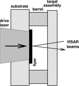
Figure 12: Schematic cross-section of laser-launched flyer impact experiments.

In the initial experiments with a Cu flyer and NiAl target, the sample covered only half of the flyer, so the flyer could be seen and its velocity measured. Several variants were used in the design of the target assembly, to investigate the accuracy of data from each. In most of these experiments, the NiAl sample was in contact with a PMMA release window; in some of the PMMA window experiments, the window was stepped to provide a more accurate measurement of the time at which impact occurred and thus the shock transit time through the sample. Experiments were also performed in which the sample was mounted on a Cu baseplate: the baseplate obscured the view of the flyer, but shock breakout at the surface of the baseplate provided a measurement of the pressure (from the peak free surface particle speed) and gave a relatively accurate measurement of the time at which the shock entered the sample. The baseplate design also avoided difficulties from light reflected from the free surface of the PMMA windows, which sometimes obscured the signal from the flyer or the sample. The baseplate had to be relatively thin to avoid decay of the shock, and the sample was not recovered from experiments using this design. (Fig. 13.)

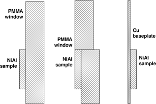
Figure 13: Schematic of target assembly for PMMA release and baseplate configurations. Center: stepped window providing better measurement of impact time. In all cases the flyer approaches from the left.

The flyer speeds were low compared with the sound speed in the target materials, so the finite accuracy of assembly – several micrometers in co-planarity or thickness – and the finite temporal registration between the point and line VISARs resulted in large uncertainties in shock transit times. The second series of experiments was designed to minimize the uncertainty in inferred particle speed and shock pressure: by using the deceleration of a NiAl flyer with a window of known properties (LiF), the Hugoniot state could be inferred from the point VISAR record only, the less precise line VISAR being used as a coarse velocity measurement (e.g. to help count fringe jumps in the point VISAR record) and to verify flatness.

V.3 Target assembly

PMMA substrates were used, coated with layers of C, Al, and Al₂O₃, in order to absorb the laser energy and insulate the flyer from heating Swift_flyeracc_05 . Cu flyers were punched from foils purchased from Goodfellow Corp. The foils had striations and machining marks which could generate interference patterns that could confuse the interpretation of the laser velocimetry records. The foils were polished manually using diamond paste to reduce the regularity of the marks. The material for the NiAl flyers was roughly triangular in shape. Rather than cutting or punching flyer disks before assembly, the triangles were attached whole to the substrates, and the drive laser punched out the central 5 mm to form the flyer. The material remaining attached to the substrate formed a seal which prevented plasma from the drive escaping radially. The barrel was much shorter than the flyer diameter, so the attachment of the edges did not make the central portion of the flyer curve measurably and did not reduce its speed.

Components were glued together with five-minute epoxy. Each flyer was clamped to its substrate while the glue set, to minimize the thickness of the glue layer. The initial viscosity of the glue was low, so the glue thickness was estimated to be negligible, essentially filling in surface irregularities. Components of the target assembly were clamped, and glued together by small drops at their corners or edges to avoid introducing any layer of glue between components which would change the shock and optical properties. (Figs 14 and 15.)

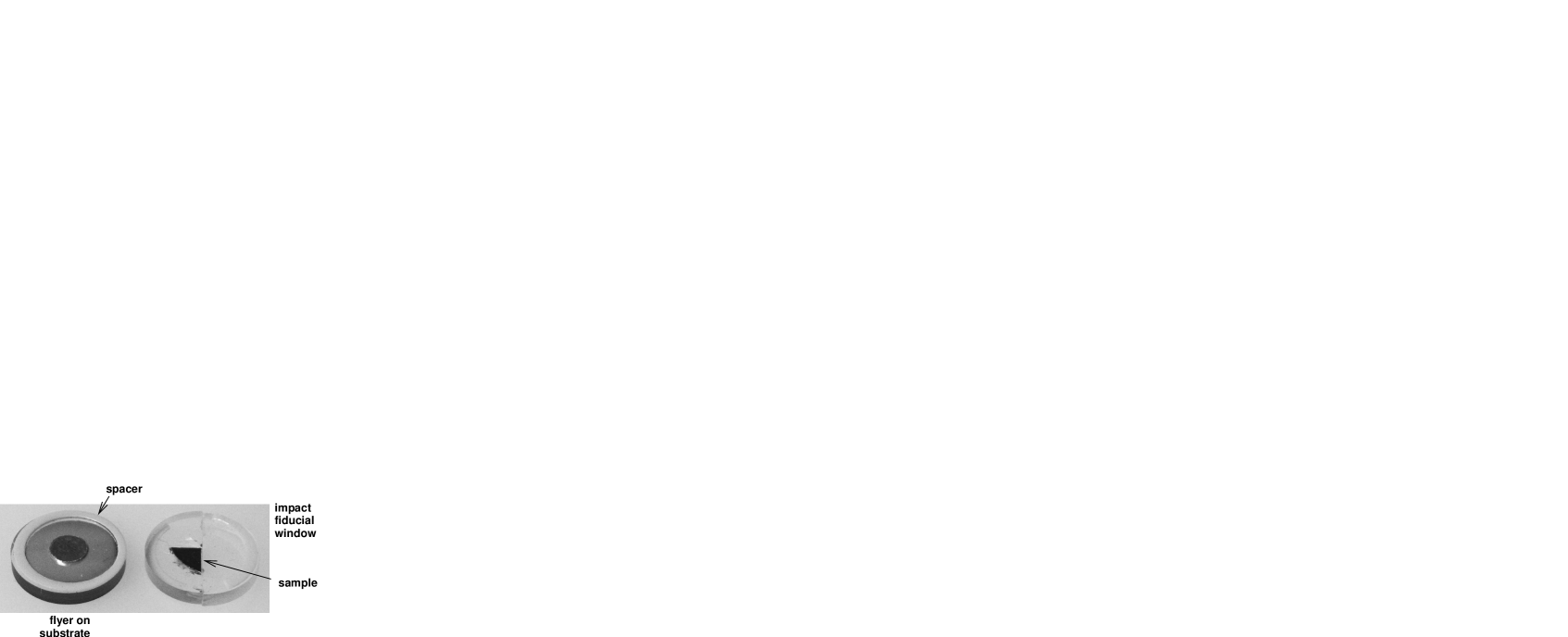
Figure 14: Example of components of shock experiment during assembly (stepped release window design). The flyer is 5 mm in diameter; the sample is visible through the window.

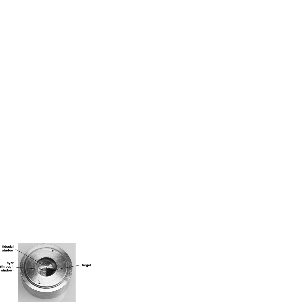
Figure 15: Example of assembled components (stepped release window design).

V.4 Diagnostics

Laser Doppler velocimetry of the ‘velocity interferometry for surfaces of any reflectivity’ (VISAR) type Barker72 was used to measure the velocity histories of the flyer and the sample. A point-VISAR and a line-imaging VISAR were used simultaneously, the point-VISAR signal being recorded on digitizing oscilloscopes and the line-VISAR signal on an optical streak camera. The point VISAR operated at a wavelength of 532 nm with a continuous-wave source, and the line VISAR at a wavelength of 660 nm with a pulsed source $\sim$1.5 $\mu$s long. Timing markers were incorporated on the streak record, at intervals of 200 ns, to provide a temporal fiducial and to allow non-linearities in camera sweep to be removed. Relative timing of the point and line VISARs was deduced by comparing the position at which a shock wave appeared in a flyer impact experiment; the relative timing had an uncertainty of $\sim$3 ns. The point VISAR was generally used to observed the NiAl.

V.5 Drive beam

The TRIDENT laser was operated in long-pulse mode, as in the previous flyer work Swift_flyeracc_05 ; Swift_NiTiEOS_05 , using an acousto-optical modulator to reduce the rate at which the pulse intensity rose and to control its shape. The drive pulse was chosen to be $\sim$600 ns long (full width, half maximum), and was delivered at the fundamental wavelength of the laser: 1054 nm (infra-red). The pulses generated were asymmetric in time, with a long tail.

An infra-red random-phase plate (RPP) was added to smooth the beam; this made a significant difference to the spatial uniformity. The beam optics were arranged to give a spot 5 mm in diameter on the substrate. The drive energy was quite low, so no RPP shield was included. The RPP collected a small amount of debris from the substrate, but was not significantly damaged.

V.6 Results

Eight experiments were performed with Cu flyers impacting NiAl, and seven with NiAl flyers impacting LiF windows (Table 3). On one shot (14138), poor fringe contrast meant that the reference velocity could not be measured by velocimetry, so it was deduced from the laser energy instead.

Table 3: Flyer impact experiments.

Shot	NiAl	Driver				Target
	orientation	thickness	speed			thickness	speed
		($\mu$m)	(m/s)			($\mu$m)	(m/s)
release window
14126	(100)	105	329	$\pm$	15	200	331	$\pm$	3
14127	(100)	105	432	$\pm$	20	217	390	$\pm$	5
14128	(100)	105	225	$\pm$	10	217	232	$\pm$	2
baseplate
14136	(100)	250	165	$\pm$	10	398	208	$\pm$	2
14137	(100)	250	200	$\pm$	10	398	260	$\pm$	2
14138	(100)	250	185	$\pm$	15	398	195	$\pm$	5
stepped disk
14139	(100)	250	153	$\pm$	2	398	120	$\pm$	10
14140	(100)	250	180	$\pm$	2	398	175	$\pm$	10
window impact
14381	(100)	94	325	$\pm$	3	-	226	$\pm$	2
14389	(100)	375	102	$\pm$	1	-	72	$\pm$	1
14390	(100)	389	152	$\pm$	3	-	107	$\pm$	3
14406	(100)	350	141	$\pm$	1	-	101	$\pm$	1
14387	(110)	228	167	$\pm$	2	-	117	$\pm$	2
14388	(110)	262	167	$\pm$	2	-	116	$\pm$	2
14405	(110)	392	149	$\pm$	2	-	106	$\pm$	1

The baseplates were 55 $\mu$m copper. The driver speed is the peak free surface speed of the baseplate, and the flyer speed on impact otherwise. The impact window was a LiF crystal, 2 mm thick, with $(100)$ planes parallel to the impact surface. The ‘target speed’ in the window impact experiments is the speed of the interface between the NiAl flyer and the LiF window immediately after impact.

The drive energy was measured with a calorimeter, and the irradiance history of the drive pulse with a photodiode. The uncertainty in energy was of the order of 1 J. The pulse shape was repeatable at the same and different energies.

The VISAR records were used to measure the velocity history and flatness of each flyer. The flyers were flat to within the accuracy of the data over the central 3 mm, with a slight lag at the edges. In some experiments, we recorded the impact of the flyer with a window and thus were able to measure the flatness directly after several hundred microns of flight. Most of the flyers were still accelerating slightly at the end of the record. There was evidence of ringing during acceleration, but no sign of shock formation or spall in the flyers.

In the release window and baseplate experiments, the velocity history at the surface of the NiAl generally exhibited a precursor to a particle speed of 15-30 m/s ahead of the main shock wave. This precursor was presumably an elastic wave. The rising part of the shock generally exhibited some structure, consistent with reverberations of the elastic wave between the surface and the approaching shock. The peak velocity was followed by deceleration of 25-30 m/s (with some outliers) and reverberations, consistent with spallation and ringing. (Figs 16 to 18.)

Figure 16: Example velocity history from a window release experiment (shot 14128).

Figure 17: Example spatially-resolved velocity history from a window release experiment (shot 14140: stepped release window).

The velocity from successive fringes has been displaced by 100 m/s for clarity.

Figure 18: Example velocity history at the free surface of the sample in a baseplate experiment (shot 14136).

In the window impact experiments, the flyer speed just before and just after impact were determined from the VISAR record (Fig. 19).

Figure 19: Example velocity histories from window impact experiments.

V.7 Analysis

The impact of a Cu flyer onto a NiAl target, releasing into a window, allowed a point on the principal Hugoniot to be deduced, relying on the assumption that the NiAl release isentrope through the shock state generated by the impact was equal to the principal Hugoniot (Fig. 20). At the pressures of a few gigapascals generated in these experiments, this assumption is accurate to a percent or better. This analysis is simplest for release into vacuum, where the particle speed in the sample can be estimated as half of the free surface speed. The difference between this and the flyer speed is equal to the particle speed in the flyer, and the Hugoniot of the flyer material can be used to find the shock pressure. Reference Hugoniots were calculated from published EOS Steinberg96 . Hugoniot states were obtained, with pressures between 2 and 8 GPa. States deduced by window release and free surface velocity were consistent. The principal Hugoniot from the ab fere initio EOS passed as closely through the data as any unique line is likely to. (Fig. 21.)

Figure 20: Schematic of construction used to deduce Hugoniot point from window release data with a flyer of known material.

Figure 21: NiAl Hugoniot points deduced from the impact of Cu flyers, compared with the ab initio equation of state.

A complication of the window impact experiments compared with the Cu flyer experiments was that the stress state at the interface between the sample and the window depends more sensitively on the elastic strain in both components. While the elastic constants may be known, the flow stress (or yield strength) is not known for all time scales. This was not such a concern for the Cu flyer experiments because the flow stress of Cu and PMMA are much lower than for LiF Steinberg96 . Calculations were made using different assumptions about the flow stress, to assess the uncertainty and the likely behavior of LiF in these experiments.

Neglecting elasticity, a measurement of the particle speed immediately before and after impact ($u_{0}$ and $u_{1}$) can be used to determine a state on the principal Hugoniot of the flyer with reference to the principal Hugoniot of the window, which must be known. Immediately after impact – for a time dictated mainly by the shock and release transit time through the flyer and window – the material in both components at the impact surface is at the same pressure and traveling at the same speed. The Hugoniots are expressed in pressure – particle speed ($p$ – $u_{p}$) space. In the shocked region, the particle velocity with respect to the undisturbed material in the window is $u_{1}$, and in the flyer $u_{0}-u_{1}$. As the same pressure exists in both materials, and it can be calculated from the Hugoniot of the window material $p_{W}(u_{1})$, a Hugoniot state can be determined in the flyer: $(u_{0}-u_{1},p_{W}(u_{1}))$. The Rankine-Hugoniot relations can then be used to calculate the other state parameters: mass density $\rho$, shock speed $u_{s}$, and the change in specific internal energy $e$ (Table 4 and Fig. 22).

Figure 22: Hugoniot points deduced for nickel – aluminum alloy, compared with the ab initio equations of state.

More rigorously, the materials at the impact interface are at the same state of normal stress $s_{11}$ rather than pressure, and under uniaxial compression. By the same arguments as above, if the shock Hugoniot of the window – now considering its response as a stress tensor $s$, at least the normal component – is known, then the normal stress of the flyer material is thus also known. The stress components for a solid depend on the elastic strain and the elastic constants. Elastic strain can be relieved by plastic flow, which limits the deviation of normal stress from the hydrostatic pressure. The elastic constants of common window materials are well-known, but the finite rate of plastic flow – which can also be considered in terms of a flow stress or yield stress which varies with strain rate – means that experiments exploring the response on different time scales may induce significantly different degrees of elastic strain for the same compression. Our experiments used flyers which were relatively thin compared with previous experiments, so it is possible that the elastic strains were somewhat greater.

Another aspect of this complication is that we ideally want to determine the EOS. Data from window impact experiments comprise the EOS plus the elastic shear stress. For a single experimental measurement in isolation, there is no way to separate the hydrostatic pressure (EOS) from the elastic stress, but some values can be extracted given data from several experiments at different pressure, and/or knowledge of the EOS or elastic and plastic behavior. In the present case, relevant complementary data include the STP elastic constants of NiAl, our QM EOS, and low strain-rate measurements of the flow stress. We considered the limiting case of no plastic flow (i.e. maximum elastic stress for a given uniaxial compression), and also cases with varying flow stresses in the window and the NiAl flyer.

For predicted shock Hugoniots including elasticity, the elastic stress was added to the Hugoniot pressure calculated from the EOS. For each state on the Hugoniot, the uniaxial compression $\eta=\rho/\rho_{0}$ was used to calculate the strain tensor (using the Green-St Venant finite strain measure Fung69 )

$$e=\left(\begin{array}[]{ccc}\frac{1}{2}\left(1/\eta^{2}-1\right)&0&0\\ 0&0&0\\ 0&0&0\end{array}\right)$$ (16)

and hence the strain deviator

$$\epsilon=\left(1-1/\eta^{2}\right)\left(\begin{array}[]{ccc}\frac{2}{3}&0&0\\ 0&\frac{1}{6}&0\\ 0&0&\frac{1}{6}\end{array}\right).$$ (17)

The corresponding elastic stress is given by

$$\frac{\partial[s]_{ij}}{\partial[e]_{kl}}=[c(\rho)]_{ijkl}$$ (18)

where $c$ is the tensor of elastic constants, strictly a function of $e$ too. In deviatoric form,

$$s\equiv\sigma(\rho,\epsilon)-p(\rho)I$$ (19)

where $p(\rho)$ is the EOS and

$$\frac{\partial[\sigma]_{ij}}{\partial[\epsilon]_{kl}}=[c(\rho)]_{ijkl}.$$ (20)

Plastic flow acts to limit the components of the elastic strain deviator $\epsilon$; in common practice it may be expressed as a constraint on the magnitude of the stress deviator.

The EOS is a more general representation of the bulk modulus

$$B=\frac{1}{3}\left(c_{11}+2c_{12}\right).$$ (21)

Comparing the response of a crystal to uniaxial compression along $[100]$, with stiffness to uniaxial compression $c_{11}$, we can define a shear modulus

$$\mu=\frac{1}{2}\left(c_{11}-c_{12}\right).$$ (22)

Using the published STP elastic constants for NiAl ($c_{11}=211.5$ GPa, $c_{12}=143.2$ GPa, $c_{44}=112.1$ GPa) Wasilewski66 , $\mu=34.2$ GPa.

The shear modulus was used to calculate the deviatoric correction to the shock Hugoniot from the EOS, for uniaxial compression. These corrections were calculated for purely elastic response, and also for different values of the flow stress $Y$ chosen to improve the match to the experimentally-measured shock states (Table 4). If the LiF window was treated as purely elastic then no treatment of the NiAl reproduced the experimental states. If the LiF was treated as elastic-plastic with flow stress $Y=0.36$ GPa as deduced from gas gun experiments, then the measured states were reproduced fairly well with a flow stress of 0.53 GPa in the NiAl. (Figs 24 and 25, also showing shock states deduced from the Cu flyer experiments. The Cu flyer data were not corrected for elastic response in the window: the correction is smaller for PMMA.)

Table 4: Shock Hugoniot states deduced from window impact experiments, using different constitutive models for LiF and NiAl.

shot	particle speed (m/s)						normal stress (GPa)
shot	for different LiF models						for different NiAl models
	hydrodynamic			$Y=0.36$ GPa			hydrodynamic			elastic			$Y=0.53$ GPa
(100)
14381	99	$\pm$	4	226	$\pm$	2	3.25	$\pm$	0.03	6.02	$\pm$	0.05	3.64	$\pm$	0.03
14389	30	$\pm$	2	72	$\pm$	1	1.00	$\pm$	0.02	1.90	$\pm$	0.03	1.39	$\pm$	0.01
14390	45	$\pm$	4	107	$\pm$	3	1.50	$\pm$	0.04	2.83	$\pm$	0.08	1.89	$\pm$	0.04
14406	40	$\pm$	2	101	$\pm$	1	1.41	$\pm$	0.01	2.67	$\pm$	0.03	1.80	$\pm$	0.01
(110)
14387	50	$\pm$	3	117	$\pm$	2	1.63	$\pm$	0.02	3.09	$\pm$	0.05	2.03	$\pm$	0.03
14388	51	$\pm$	4	116	$\pm$	2	1.62	$\pm$	0.02	3.07	$\pm$	0.05	2.01	$\pm$	0.03
14405	43	$\pm$	2	106	$\pm$	1	1.48	$\pm$	0.02	2.80	$\pm$	0.03	1.87	$\pm$	0.01

The hydrodynamic model for NiAl was used with the hydrodynamic model for LiF. The elastic and elastic-plastic models for NiAl were used with the elastic-plastic model for LiF.

Figure 23: Stress states deduced for NiAl, using different assumptions about plasticity in the LiF window.

Figure 24: Hugoniot points deduced for NiAl, compared with the ab initio equation of state. Points with large error bars are from the Cu flyer experiments.

Figure 25: Hugoniot points deduced for NiAl, compared with the ab initio equation of state. Points with large error bars are from the Cu flyer experiments.

The precursor waves and the deceleration following the peak of the shock can be used to infer flow stresses and spall strengths. However, simple models parameterized from these data can be misleading, so the detailed constitutive behavior of NiAl will be reported separately in the context of microstructural response. The true (i.e. normal) stress to induce plastic flow at lower strain rates has been reported at around 1.5 GPa Maloy95 , corresponding to a flow stress of around 0.4 GPa. One would expect the stresses to be at least as large on the shorter time scales of the laser experiments, so the flow stress inferred from the window impact experiments is quite plausible.

VI Conclusions

The frozen-ion compression curve for NiAl in the CsCl structure was predicted using ab initio quantum mechanical calculations of the electron band structure. The calculations reproduced the lattice parameter at $p=0$ to $\sim$1% with no corrections, equivalent to a discrepancy $\sim 7$ GPa. The ab initio pressure-volume relation calculated using the Hellmann-Feynman theorem was not perfectly consistent with the ab initio energy-volume relation; this reflects the lower precision of the stress calculations. The Rose functional form, found to fit the energy-volume relation for compression of a wide range of elements, was found to fit the energy-volume relation for compression of NiAl, but deviated significantly in expansion. The electron band structure was used to predict electron-thermal excitations. The mechanical response in the equation of state and shock Hugoniot did not alter much when the electron-thermal contribution was included, though the Hugoniot pressure-temperature relation varied by around 1% per thousand kelvin. The charge distribution in the electron ground states was used to predict ab initio phonon modes, from the forces on the atoms when one was displaced from equilibrium. The phonon density of states was quite sensitive to the magnitude of the displacement – though the restoring force on the displaced atom itself suggested that the effective potential it experienced was essentially harmonic – but thermodynamically-complete equations of state constructed using the phonon modes were not sensitive to the details of the density of phonon states up to $\sim$100 GPa. The quasiharmonic equations of state reproduced published measurements of isothermal compression of NiAl extremely well, and were also consistent with measurements of the shock compression.

Laser-driven flyer experiments were performed to measure states on the principal shock Hugoniot of NiAl, by impacting Cu flyers into NiAl targets and by impacting NiAl flyers against LiF windows. Shock transit times were not measured accurately enough to constrain the EOS. Shock states from the Cu flyer data were obtained with respect to the Hugoniot of Cu or PMMA. These states were consistent with the ab initio EOS for NiAl. Detailed interpretation of the NiAl flyer data depends on the elastic-plastic behavior of the NiAl and the LiF. Ignoring these elastic contributions, the shock states were consistent with theoretical EOS. If the LiF was assumed to response elastically, the stress states deduced were implausibly high. If it was assumed to response with the same flow stress as observed in gas gun experiments – which typically explore somewhat longer time scales – then it was possible to reproduce the shock states by taking either EOS and adjusting the flow stress in the NiAl. Reasonable agreement was obtained for the quasiharmonic EOS with a flow stress of 0.53 GPa, which is consistent with the range of values deduced from the amplitude of the elastic precursor wave in other shock loading experiments. The quasiharmonic EOS – which was found to reproduce quasistatic compression data extremely well – is thus consistent with the shock measurements.

References

- (1) J.A. Moriarty, High Pressure Research 13, 6 (1995).
- (2) B. Militzer and D.M. Ceperley, Phys. Rev. E 63, 6, 066404-10 (2001).
- (3) P. Hohenberg and W. Kohn, Phys. Rev. B 136, 3B (1964).
- (4) W. Kohn and L.J. Sham, Phys. Rev. 140, 4A (1965).
- (5) J.P. Perdew, J.A. Chevary, S.H. Vosko, K.A. Jackson, M.R. Pederson, D.J. Singh, and C. Fiolhais, Phys. Rev. B 46, 6671 (1992).
- (6) J.A. White and D.M. Bird, Phys. Rev. B 50, R4954 (1994).
- (7) N.W. Ashcroft and N.D. Mermin, “Solid State Physics” (Holt-Saunders, New York, 1976).
- (8) B.I. Bennett and D.A. Liberman, INFERNO, Los Alamos National Laboratory report LA-10309-M (1985).
- (9) D.A. Liberman and B.I. Bennett, Phys. Rev. B 42, 2475 (1990).
- (10) J.S. Dugdale and D.K.C. McDonald, Phys. Rev. 89, 832 (1953).
- (11) J.D. Kress, S. Mazevet, and L.A. Collins, Contrib. Plasma Phys. 41, 2-3, pp 139-42 (2001).
- (12) D.C. Swift, G.J. Ackland, A. Hauer, and G.A. Kyrala, Phys. Rev. B 64, 214107, (2001).
- (13) D.C. Swift, R.E. Hackenberg, J.G. Niemczura, G.J. Ackland, J. Cooley, D.L. Paisley, R.P. Johnson, A. Hauer, and D. Thoma, J. Appl. Phys. 98, 093512 (2005).
- (14) G.J. Ackland, X. Huang, and K.M. Rabe, Phys. Rev. B 68, 214104 (2003).
- (15) G.J. Ackland, J. Phys.: Cond. Matt. 14, 2975 (2002).
- (16) N. Troullier and J.L. Martins, Phys. Rev. B 43, pp 1993-2006 (1991).
- (17) G.J. Ackland, M.C. Warren and S.J. Clark, J. Phys.: Cond. Matt. 9, 7861 – 7872 (1997).
- (18) D.B. Miracle, Acta Metall. Mater. 41, 3, 649 – 684 (1993).
- (19) H.J. Monkhorst and J.D. Pack, Phys. Rev. B 13, 5188 (1976).
- (20) P. Pulay, Mol. Phys. 17, 197 (1969).
- (21) G.P. Francis and M.C. Payne, J. Phys. C 2, 4395 (1990).
- (22) M.C. Warren and G.J. Ackland, Physics and Chemistry of Materials 23, 2 (1996).
- (23) H.C. Hsueh, M.C. Warren, H. Vass, G.J. Ackland, S.J. Clark and J. Crain, Phys. Rev. B 53, 14806 (1996).
- (24) J.J. Rose, J.R. Smith, F. Guinea, and J. Ferrante, Phys. Rev. B 29, 2963 (1984).
- (25) A.P. Sutton, “Electronic Structure of Materials” (Oxford University Press, Oxford, 1993).
- (26) R.F. Trunin, “Shock Compression of Condensed Materials” (Cambridge University Press, Cambridge, 1998).
- (27) C. Kittel, “Introduction to solid state physics” (Wiley, New York, 1996).
- (28) Maradudin, Montroll, and Weiss, “Theory of Lattice Dynamics in the Harmonic Approximation” (Academic Press, New York, 1963).
- (29) X.-Y. Huang, I.I. Naumov, and K.M. Rabe, Phys. Rev. B 70, 064301 (2004).
- (30) U. Pinsook and G.J. Ackland, Phys. Rev. B 59, 13642-13649 (1999).
- (31) N.D. Drummond and G.J. Ackland, Phys. Rev. B 65, 184104 (2001).
- (32) Y. Wang, Z.-K. Liu, and L.-Q. Chen, Acta Materialia 52, 2665-71 (2004).
- (33) S.P. Lyon and J.D. Johnson (Los Alamos National Laboratory), SESAME: the Los Alamos National Laboratory equation of state database, Los Alamos National Laboratory report LA-UR-92-3407 (1992).
- (34) J.W. Otto, J.K. Vassiliou, and G. Frommeyer, J. Mater. Res. 12, 11, 3106-8 (1997).
- (35) R.J. Wasilewski, Trans. Metallurgical Soc. of AIME 236, pp 455-7 (1966).
- (36) A.V. Bushman, G.I. Kanel’, A.L. Ni, and V.E. Fortov, “Intense Dynamic Loading of Condensed Matter” (Taylor and Francis, London, 1993).
- (37) D.C. Swift, J.G. Niemczura, D.L. Paisley, R.P. Johnson, S.-N. Luo, and T.E. Tierney, Rev. Sci. Instrum. 76, 093907 (2005).
- (38) L.M. Barker and R.E. Hollenbach, J. Appl. Phys. 43, 4669 (1972).
- (39) D.J. Steinberg, Equation of state and strength properties of selected materials, Lawrence Livermore National Laboratory report UCRL-MA-106439 change 1 (1996).
- (40) Y.C. Fung, “A First Course in Continuum Mechanics” (Prentice-Hall, New York, 1969).
- (41) S.A. Maloy, G.T. Gray III, and R. Darolia, Materials Sci. and Eng. A192/193, pp 249-54 (1995).