Particle Motion Around Tachyon Monopole

Abstract

Recently, Li and Liu have studied global monoole of tachyon in a four dimensional static space-time. We analyze the motion of massless and massive particles around tachyon monopole. Interestingly, for the bending of light rays due to tachyon monopole instead of getting angle of deficit we find angle of surplus. Also we find that the tachyon monopole exerts an attractive gravitational force towards matter.

1. Introduction:

At the early stages of its evolution, the Universe has underwent a number of phase transitions. During the phase transitions, the symmetry has been broken. According to the Quantum field theory, these types of symmetry-breaking phase transitions produces topological defects [1]. These are namely domain walls, cosmic strings, monopoles and textures. Monopoles are point like defects that may arise during phase transitions in the early universe. In particular , $\pi_{2}(M)\neq I$ ( M is the vacuum manifold ) i.e. M contains surfaces which can not be continuously shrunk to a point, then monopoles are formed [2].
A typical symmetry - breaking model is described by the Lagrangian,

$$L=\frac{1}{2}\partial_{\mu}\Phi^{a}\partial^{\mu}\Phi^{a}-V(f)$$ (1)

Where $\Phi^{a}$ is a set of scalar fields, $a=1,2,..,N,f=\sqrt{\Phi^{a}\Phi^{a}}$ and $V(f)$ has a minimum at a non zero value of $f$. The model has $0(N)$ symmetry and admits domain wall, string and monopole solutions for $N=1,2$ and $3$ respectively. It has been recently suggested by Cho and Vilenkin(CV) [3,4] that topological defects can also be formed in the models where $V(f)$ is maximum at $f=0$ and it decreases monotonically to zero for $f\rightarrow\infty$ without having any minima. For example,

$$V(f)=\lambda M^{4+n}(M^{n}+f^{n})^{-1}$$

where $M,\lambda$ and $n$ are positive constants. This type of potential can arise in non-perturbative superstring models. Defects arising in these models are termed as ” vacuumless defects ”. Recently, several authors have studied vacuumless topological defects in alternative theory of gravity [5].

Barriola and Vilenkin [6] were the pioneer who studied the gravitational effects of global monopole. It was shown by considering only gravity that the linearly divergent mass of global monopole has an effect analogous to that of a deficit solid angle plus that of a tiny mass at the origin [6]. Later it was studied by Harari and Loustò [7], and Shi and Li [8] that this small gravitational potential is actually repulsive. Recently, Sen [9] showed in string theories that classical decay of unstable D-brane produces pressureless gas which has non-zero energy density. The basic idea is that though the usual open string vacuum is unstable, there exists a stable vacuum with zero energy density.This state is associated with the condensation of electric flux tubes of closed string [10]. By using an effective Born-Infeld action, these flux tubes could be explained [11]. Sen also proposed the tachyon rolling towards its minimum at infinity as a dark matter candidate [10]. Sen have also analyzed the Dirac-Born-Infeld Action on the Tachyon Kink and Vortex[12]. Gibbons actually initiated the study of tachyon cosmology . He took the coupling into gravitational field by adding an Einstein-Hilbert term to the effective action of the tachyon on a brane [13]. In the cosmological background, several scientists have studied the process of rolling of the tachyon [14, 15].

Different kinds of cold stars such as Q-stars have been proposed to be a candidate for the cold dark matter [16-25]. A new class of cold stars named as D-stars(defect stars) have been proposed by Li et.al.[26]. Compared to Q-stars, the D-stars have a peculiar phenomena, that is, in the absence of the matter field the theory has monopole solutions, which makes the D-stars behave very differently from the Q-stars. Moreover, if the universe does not inflate and the tachyon field T rolls down from the maximum of its potential, the quantum fluctuations produced various topological defects during spontaneous symmetry breaking. That is why it is so crucial to investigate the property and the gravity of the topological defects of tachyon, such as Vortex [27], Kink [28] and monopole, in the static space time. Recently, Li and Liu [29] have studied gravitational field of global monopole of tachyon.

In this paper, we will discuss the behavior of the motion of massless and massive particles around Tachyon Monopole. We will calculate the amount of deficit angle for the bending of light rays. Also we will investigate the nature of gravitational field of tachyon monopole towards matters by using Hamilton-Jacobi method.

2. Tachyon Monopole Revisited:

Let us consider, a general static, spherically-symmetric metric as

$$ds^{2}=A(r)dt^{2}-B(r)dr^{2}-r^{2}(d\theta^{2}+sin^{2}\theta d\phi^{2})$$ (2)

The Lagrangian density of rolling tachyon can be written in Born-Infeld form as

$$L=L_{R}+L_{T}=\sqrt{-g}\left[\frac{R}{2\kappa}-V(|T|)\sqrt{1-g^{\mu\nu}\partial_{\mu}T^{a}\partial_{\nu}T^{a}}\right]$$

where $T^{a}$ is a triplet of tachyon fields, $a=1,2,3$ and $g_{\mu\nu}$ is the metric coefficients. One can consider the monopole as associated with a triplet of scalar field as

$$T^{a}=f(r)\frac{x^{a}}{r}$$

where $x^{a}x^{a}=r^{2}$. Now using the Lagrangian density, L, the metric and the scalar field, the Einstein equations take the following forms as

$$\frac{1}{r^{2}}-\frac{1}{B}\left(\frac{1}{r^{2}}+\frac{B^{\prime}}{rB}\right)=\kappa T^{0}_{0}$$

$$\frac{1}{r^{2}}-\frac{1}{B}\left(\frac{1}{r^{2}}+\frac{A^{\prime}}{rA}\right)=\kappa T^{1}_{1}$$

where the prime denotes the derivative with respect to r and energy momentum tensor $T^{\mu}_{\nu}$ are given by

$$T^{0}_{0}=V(f)\sqrt{1+\frac{f^{\prime 2}}{B}+\frac{2f^{2}}{r^{2}}}$$

$$T^{1}_{1}=\frac{V(f)(1+\frac{2f^{2}}{r^{2}})}{\sqrt{1+\frac{f^{\prime 2}}{B}+\frac{2f^{2}}{r^{2}}}}$$

$$T^{2}_{2}=T^{3}_{3}=\frac{V(f)(1+\frac{f^{\prime 2}}{B}+\frac{f^{2}}{r^{2}})}{\sqrt{1+\frac{f^{\prime 2}}{B}+\frac{2f^{2}}{r^{2}}}}$$

and the rest are zero. So, the system depends on the tachyon potential $V(T)$. According to Sen [9], the potential should have an unstable maximum at $T=0$ and decay exponentially to zero when $T\rightarrow\infty$.

One can choose the tachyon potential which satifies the above two conditions as follows:

$$V(f)=M^{4}\left(1+3\lambda f^{4}\right)^{\frac{1}{6}}exp(-\lambda f^{4})$$

where $M$ and $\lambda$ are positive constants.

In flat space-time, the Euler-Lagrange equation will take the following form:

$$\frac{1}{V}\left(\frac{dV}{df}\right)+\frac{2f}{r^{2}}=f^{\prime\prime}+\frac{2f^{\prime}}{r}-f^{\prime}\left[\frac{f^{\prime}f^{\prime\prime}+\frac{2f}{r^{2}}\left(f^{\prime}-\frac{f}{r}\right)}{1+f^{\prime 2}+\frac{2f^{2}}{r^{2}}}\right]$$

and the energy density of the system can be written as

$$T^{0}_{0}=V(f)\sqrt{1+f^{\prime 2}+\frac{2f^{2}}{r^{2}}}$$

For the above mentioned tachyon potential, $V(f)$ the Euler-Lagrange equation has a simple exact solution

$$f(r)=\lambda^{-\frac{1}{4}}\left(\frac{\delta}{r}\right)$$

where $\delta=\lambda^{-\frac{1}{4}}$ is the size of the monopole core and corresponding energy density becomes

$$T^{0}_{0}=M^{4}\left[1+3\left(\frac{\delta}{r}\right)^{4}\right]^{\frac{2}{3}}exp\left[-\left(\frac{\delta}{r}\right)^{4}\right]$$

Considering the Newtonian approximation, the Newtonian potential can be written as

$$\nabla^{2}\Phi=\frac{\kappa}{2}(T^{0}_{0}-T^{i}_{i})$$

At $r\gg\delta$,

$$T^{0}_{0}-T^{i}_{i}\simeq-2M^{4}.$$

Therefore, the solution of the above equation is

$$\Phi(r)\simeq-\frac{4\pi M^{4}}{3\lambda M_{p}^{2}f^{2}}$$

where $M_{p}$ is the Planck mass and the parameter M should satisfies the condition $M\leq 10^{-3}$ eV in order to avoid conflicting present cosmological observations. The linearized approximation applies for $|\Phi(r)|\ll 1$, which is equivalent to $f\gg\sqrt{\frac{4\pi}{3\lambda}}\frac{M^{2}}{M_{p}}$.

Now, one can express the metric coefficients A(r) and B(r) as

$$A(r)=1+\alpha(r),B(r)=1+\beta(r).$$

Linearizing in $\alpha(r)$ and $\beta(r)$, and using the flat space expression for $f(r)$, the Einstein equations becomes

$$\frac{\alpha^{\prime}}{r}+\frac{\beta^{\prime}}{r}=\kappa M^{4}\left(\frac{\delta}{r}\right)^{4}\left[1+3\left(\frac{\delta}{r}\right)^{4}\right]^{-\frac{1}{3}}exp\left[-\left(\frac{\delta}{r}\right)^{4}\right]$$

and

$$\alpha^{\prime\prime}+\frac{2\alpha^{\prime}}{r}=-\kappa M^{4}\left[2+3\left(\frac{\delta}{r}\right)^{4}\right]\left[1+3\left(\frac{\delta}{r}\right)^{4}\right]^{-\frac{1}{3}}exp\left[-\left(\frac{\delta}{r}\right)^{4}\right]$$

After solving one can write the solution of the external metric as

$$A(r)=\left(1-\frac{\kappa M^{4}}{3}r^{2}\right);B(r)=\left(1+\frac{\kappa M^{4}}{3}r^{2}-\frac{\kappa M^{4}}{2\lambda r^{2}}\right)$$ (3)

3. The Geodesics:

Let us now write down the equation for the geodesics in the metric (2) . From

$$\frac{d^{2}x^{\mu}}{d\tau^{2}}+\Gamma^{\mu}_{\nu\lambda}\frac{dx^{\nu}}{d\tau}\frac{dx^{\lambda}}{d\tau}=0$$ (4)

we have

$$B(r)\left(\frac{dr}{d\tau}\right)^{2}=\frac{E^{2}}{A(r)}-\frac{J^{2}}{r^{2}}-L$$ (5)

$$r^{2}\left(\frac{d\phi}{d\tau}\right)=J$$ (6)

$$\frac{dt}{d\tau}=\frac{E}{A(r)}$$ (7)

where the motion is considered in the $\theta=\frac{\pi}{2}$ plane and constants E and J are identified as the energy per unit mass and angular momentum, respectively , about an axis perpendicular to the invariant plane $\theta=\frac{\pi}{2}$. Here $\tau$ is the affine parameter and L is the Lagrangian having values 0 and 1, respectively, for massless and massive particles.
The equation for radial geodesic ( $J=0$):

$$\dot{r}^{2}\equiv\left(\frac{dr}{d\tau}\right)^{2}=\frac{E^{2}}{A(r)B(r)}-\frac{L}{B(r)}$$ (8)

Using equation(7) we get

$$\left(\frac{dr}{dt}\right)^{2}=\frac{A(r)}{B(r)}-\frac{A^{2}(r)L}{E^{2}B(r)}$$ (9)

From equation(3), we can write

$$\left(\frac{dr}{dt}\right)^{2}=\left(1-\frac{\kappa M^{4}}{3}r^{2}\right)\left(1+\frac{\kappa M^{4}}{3}r^{2}-\frac{\kappa M^{4}}{2\lambda r^{2}}\right)^{-1}-\frac{L}{E^{2}}\left(1+\frac{\kappa M^{4}}{3}r^{2}-\frac{\kappa M^{4}}{2\lambda r^{2}}\right)^{-1}\left(1-\frac{\kappa M^{4}}{3}r^{2}\right)^{2}$$ (10)

Expanding the expression binomially and neglecting the higher order of $\kappa M^{4}$ ( as $\kappa M^{4}$ is very small ) we get

$$\left(\frac{dr}{dt}\right)^{2}=\left(1-\frac{2\kappa M^{4}}{3}r^{2}+\frac{\kappa M^{4}}{2\lambda r^{2}}\right)-\frac{L}{E^{2}}\left(1-\kappa M^{4}r^{2}+\frac{\kappa M^{4}}{2\lambda r^{2}}\right)$$ (11)

3.1. Motion of Massless Particle ( L=0 ): In this case,

$$\left(\frac{dr}{dt}\right)^{2}=\left(1-\frac{2\kappa M^{4}}{3}r^{2}+\frac{\kappa M^{4}}{2\lambda r^{2}}\right)$$ (12)

After integrating, we get

$$\pm t=\int\frac{rdr}{\sqrt{\left(r^{2}-\frac{2\kappa M^{4}}{3}r^{4}+\frac{\kappa M^{4}}{2\lambda}\right)}}$$ (13)

This gives the $t-r$ relationship as

$$\pm t=-\frac{1}{\sqrt{\frac{8\kappa M^{4}}{3}}}sin^{-1}\left(\frac{1-\frac{4\kappa M^{4}}{3}r^{2}}{\sqrt{1+\frac{4\kappa^{2}M^{8}}{3\lambda}}}\right)$$ (14)

The $t-r$ relationship is depicted in Fig. 1.

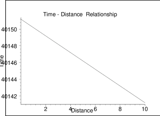
Figure 1: $t-r$ relationship for massless particle( choosing $\kappa M^{4}=573.95\times 10^{-12}$, $\lambda=1$ )

Again, from equation (8) we get

$$\dot{r}^{2}\equiv\left(\frac{dr}{d\tau}\right)^{2}=\frac{E^{2}}{A(r)B(r)}$$ (15)

After integrating, we get

$$\pm E\tau=\int\sqrt{\left(1-\frac{\kappa M^{4}}{3}r^{2}\right)\left(1+\frac{\kappa M^{4}}{3}r^{2}-\frac{\kappa M^{4}}{2\lambda r^{2}}\right)}dr$$ (16)

This gives the $\tau-r$ relationship as

$$\pm E\tau=\left(r+\frac{\kappa M^{4}}{4\lambda r}\right)$$ (17)

( neglecting the higher order of $\kappa M^{4}$ ).

We show graphically (see Fig. 2 ) the variation of proper-time ($\tau$) with respect to radial co-ordinates (r) .

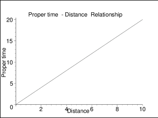
Figure 2: $\tau-r$ relationship for massless particle ( choosing $\kappa M^{4}=573.95\times 10^{-12}$, $\lambda=1,E=0.5$ )

3.2. Motion of Massive Particles ( L=1 ): In this case,

$$\left(\frac{dr}{dt}\right)^{2}=\left(1-\frac{2\kappa M^{4}}{3}r^{2}+\frac{\kappa M^{4}}{2\lambda r^{2}}\right)-\frac{1}{E^{2}}\left(1-\kappa M^{4}r^{2}+\frac{\kappa M^{4}}{2\lambda r^{2}}\right)$$ (18)

After integrating, we get

$$\pm t=\int\frac{Erdr}{\sqrt{\left(\kappa M^{4}-\frac{2\kappa M^{4}E^{2}}{3}\right)r^{4}+\left(E^{2}-1\right)r^{2}+\frac{\kappa M^{4}}{2\lambda}\left(E^{2}-1\right)}}$$ (19)

This gives the $t-r$ relationship as (see graphical Fig. (3))

$\pm t=\frac{E/2}{\sqrt{\kappa M^{4}\left(1-\frac{2}{3}E^{2}\right)}}\ln[2\sqrt{\left(\kappa M^{4}\left(1-\frac{2}{3}E^{2}\right)\right)\left(\kappa M^{4}\left(1-\frac{2}{3}E^{2}\right)r^{4}\right)+\left(E^{2}-1\right)r^{2}+\frac{\kappa M^{4}}{2\lambda}\left(E^{2}-1\right)}\linebreak+2\kappa M^{4}\left(1-\frac{2}{3}E^{2}\right)r^{2}+\left(E^{2}-1\right)]$

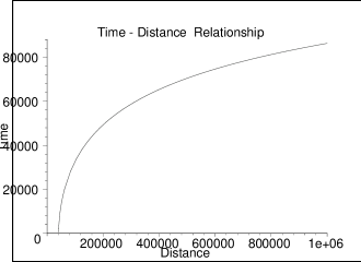
Figure 3: $t-r$ relationship for massive particle( choosing $\kappa M^{4}=573.95\times 10^{-12}$, $\lambda=1,E=0.5$ )

Again, from equation (8) we get

$$\dot{r}^{2}\equiv\left(\frac{dr}{d\tau}\right)^{2}=\frac{E^{2}}{A(r)B(r)}-\frac{1}{B(r)}$$

Neglecting the higher order of $\kappa M^{4}$ , we get

$$\pm\int d\tau=\int\frac{\left(1-\frac{\kappa M^{4}}{4\lambda r^{2}}\right)dr}{\sqrt{E^{2}-1+\frac{\kappa M^{4}}{3}r^{2}}}$$

This gives the $\tau-r$ relationship as

$$\pm\tau=\sqrt{\frac{3}{\kappa M^{4}}}\cosh^{-1}\left[\frac{r}{\sqrt{\frac{3(1-E^{2})}{\kappa M^{4}}}}\right]-\frac{(\kappa M^{4})^{3/2}}{4\sqrt{3}\lambda(1-E^{2})}\frac{\sqrt{r^{2}-\frac{3(1-E^{2})}{\kappa M^{4}}}}{r}$$

We show graphically (see Fig. 4 ) the variation of proper-time ($\tau$) with respect to radial co-ordinates (r) .

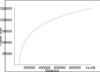
Figure 4: $\tau-r$ relationship for massive particle ( choosing $\kappa M^{4}=573.95\times 10^{-12}$, $\lambda=1,E=0.5$ )

4. Bending of Light rays:

For photons ( L=0 ), the trajectory equations (5) and (6) yield

$$\left(\frac{dU}{d\phi}\right)^{2}=\frac{a^{2}}{A(r)B(r)}-\frac{U^{2}}{B(r)}$$ (20)

where $U=\frac{1}{r}$ and $a^{2}=\frac{E^{2}}{J^{2}}$.

Equation (20) and (3) gives

$$\phi=\int\frac{\pm dU}{\sqrt{\left(a^{2}+\frac{\kappa M^{4}}{3}\right)-\left(1-\frac{a^{2}\kappa M^{4}}{2\lambda}\right)U^{2}}}$$ (21)

( neglecting the higher order of $\kappa M^{4}$ and the product of $\kappa M^{4}$ $\times$$U^{4}$ terms ).
This gives

$$\phi=\frac{1}{\sqrt{\left(1-\frac{a^{2}\kappa M^{4}}{2\lambda}\right)}}cos^{-1}\frac{U}{A}$$ (22)

where $A=\frac{a^{2}+\frac{\kappa M^{4}}{3}}{1-\frac{a^{2}\kappa M^{4}}{2\lambda}}$.

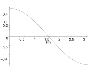
Figure 5: We Plot U vs. $\phi$ ( choosing $\kappa M^{4}=573.95\times 10^{-12}$, $\lambda=1,a^{2}=0.5$)

For $U\rightarrow 0$, one gets

$$2\phi=\pi\left(1+\frac{a^{2}\kappa M^{4}}{4\lambda}\right)$$ (23)

and bending comes out as

$$\Delta\phi=\pi-2\phi=\pi-\pi\left(1+\frac{a^{2}\kappa M^{4}}{4\lambda}\right)=-\frac{a^{2}\kappa M^{4}}{4\lambda}\pi$$ (24)

which is nothing but angle of surplus[30].

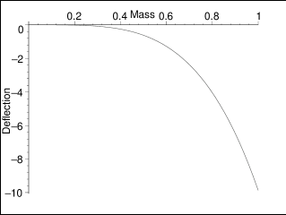
Figure 6: We plot Deflection vs. Mass ( choosing $\kappa=25.12$, $\lambda=1,a^{2}=0.5$ )

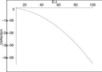
Figure 7: We plot Deflection vs. E/J ( choosing $\kappa M^{4}=573.95\times 10^{-12}$,$\lambda=1$ )

5. Motion of test particle:

Let us consider a test particle having mass $m_{0}$ moving in the gravitational field of the tachyon monopole described by the metric ansatz(2). So the Hamilton-Jacobi [ H-J ] equation for the test particle is [31]

$$g^{ik}\frac{\partial S}{\partial x^{i}}\frac{\partial S}{\partial x^{k}}+m_{0}^{2}=0$$ (25)

where $g_{ik}$ are the classical background field (2) and S is the standard Hamilton’s characteristic function .

For the metric (2) the explicit form of H-J equation (25) is [31]

$$\frac{1}{A(r)}\left(\frac{\partial S}{\partial t}\right)^{2}-\frac{1}{B(r)}\left(\frac{\partial S}{\partial r}\right)^{2}-\frac{1}{r^{2}}\left(\frac{\partial S}{\partial\theta}\right)^{2}-\frac{1}{r^{2}\sin^{2}\theta}\left(\frac{\partial S}{\partial\varphi}\right)^{2}+m_{0}^{2}=0$$ (26)

where $A(r)$ and $B(r)$ are given in equation (3) .

In order to solve this partial differential equation, let us choose the $H-J$ function $S$ as [32]

$$S=-E.t+S_{1}(r)+S_{2}(\theta)+J.\varphi$$ (27)

where $E$ is identified as the energy of the particle and $J$ is the momentum of the particle.

The radial velocity of the particle is ( for detailed calculations, see $ref.[32]$ )

$$\frac{dr}{dt}=\frac{A(r)}{E\sqrt{B(r)}}\sqrt{\frac{E^{2}}{A(r)}+m_{0}^{2}-\frac{p^{2}}{r^{2}}}$$ (28)

where $p$ is the separation constant.

The turning points of the trajectory are given by $\left(\frac{dr}{dt}\right)=0$ and as a consequence the potential curve are

$$\frac{E}{m_{0}}=\sqrt{A(r)\left(\frac{p^{2}}{m_{0}^{2}r^{2}}-1\right)}\equiv V(r)$$ (29)

In a stationary system, $E$ i.e. $V(r)$ must have an extremal value. Hence the value of $r$ for which energy attains it extremal value is given by the equation

$$\frac{dV}{dr}=0$$ (30)

Hence we get

$$\frac{2\kappa M^{4}}{3}r^{4}=\frac{2p^{2}}{m^{2}}\Rightarrow r=\left(\frac{3p^{2}}{\kappa M^{4}m^{2}}\right)^{\frac{1}{4}}$$ (31)

So this equation has at least one positive real root. Therefore, it is possible to have bound orbit for the test particle i.e. the test particle can be trapped by the tachyon monopole. In other words, the tachyon monopole exerts an attractive gravitational force towards matter.

6. Concluding remarks:

In this paper, we have investigated the behavior of a massless and massive particles in the gravitational field of a tachyon monopole. The tachyon monopole, in compare to the ordinary monopole, are very diffuse objects whose energy distributed at large distances from the monopole core, their space-time is vastly different from the ordinary monopole. The figures (1) and (2) indicate that the nature of ordinary time and proper time for the massless particle in the gravitational field of tachyonic monopole is opposite to each other. Here, one can see that ordinary time decreases with increase of radial distance where as the proper time increases with increase of radial distance. Figures (3) and (4) show that in case of massive particle, the ordinary time and proper time have the same nature. According to Li and Liu [29], tachyon monopole has a small gravitational potential of repulsive nature, corresponding to a negative mass at origin. In the analysis of the bending of light rays, we get angle of surplus instead of angle of deficit. So, we may conclude that it has a property of short range repulsive force. From eqn.(31), we see that $r=\frac{1}{M}\left(\frac{3p^{2}}{\kappa m^{2}}\right)^{\frac{1}{4}}$ i.e. $r$ would be very large as $M$ is very small, in other words, particle can be trapped at a large distance from the monopole core. This implies tachyon monopole would have effect on particles far away from its core. That means tachyon monopole has a long range gravitational field which is sharply contrast to ordinary monopole.

Acknowledgments

F.R. is thankful to DST , Government of India for providing financial support. MK has been partially supported by UGC, Government of India under MRP scheme.

References

[1] T.W.B. Kibble, J. Phys. A9, 1387(1976).
[2] A. Vilenkin and E.P.S. Shellard Cosmic String and other Topological
Defects (Camb. Univ. Press) (1994).
[3] I. Cho and A. Vilenkin, Phys.Rev.D59, 021701(1999).
[4] I. Cho and A. Vilenkin, Phys.Rev.D59, 063510(1999).
[5] F. Rahaman et al, arXiv: gr-qc/0610086; F. Rahaman et al, Fizika B12, 291(2003); A.A. Sen, Int.J.Mod.Phys.D10, 515(2001);
L.C. Garcia de Andrade, arXiv: gr-qc/9902078; F. Rahaman et al, arXiv: gr-qc/0702147.
[6] M. Barriola and A. Vilenkin, Phys. Rev. Lett.63, 341(1989).
[7] D. Harari and C. Loustò, Phys. Rev. D42, 2626(1990).
[8] X. Shi and X. Z. Li, Class. Quantum Grav. 8, 761(1991).
[9] A. Sen, JHEP 9806, 007(1998); A. Sen, JHEP 9808, 010(1998); A. Sen, JHEP 9808, 012(1998).
[10] A. Sen, JHEP 0204, 048(2002); A. Sen, JHEP 0207, 065(2002).
[11] A. Sen J. Math. Phys. 42, 2844(2001); G. W. Gibbons, K. Hori and P. Yi, Nucl. Phys. B596, 136(2001).
[12] A. Sen, Phys.Rev. D68, 066008(2003).
[13] G. W. Gibbons, Phys. Lett. B537, 1(2002);
M. Sami and T. Padmanabhan Phys. Rev. D67, 083509(2003).
[14] X. Z. Li, J. G. Hao and D. J. Liu, Chin. Phys. Lett. 19, 1584(2002); J. G. Hao and X. Z. Li, Phys. Rev. D66, 087301(2002);
J. G. Hao and X. Z. Li, Phys. Rev. D68, 067501(2003); D. J. Liu and X. Z. Li, Phys. Rev. D70, 123504(2004);
J. G. Hao and X. Z. Li, Phys. Rev. D70, 043529(2004).
[15] M. Sami, P. Chingangbam, T. Qureshi, Phys.Rev. D66, 043530(2002); D. Choudhury et al, Phys.Lett. B544, 231(2002);
X. Z. Li and X. H. Zhai, Phys. Rev.D67, 067501(2003); S. Mukohyama, Phys. Rev. D66, 123512(2002);
J. S. Bagla, H. K. Jassal and T. Padmanabhan,Phys. Rev. D67, 063504(2003); T. Padmanabhan, Phys. Rept. 380, 235(2003);
P. Singh, M. Sami, N. Dadhich, Phys. Rev. D68, 023522(2003).
[16] R. Ruffini and S. Binazzola, Phys.Rev. 187, 1767(1969).
[17] M. Colpi, S.L. Shapiro and I. Wasserman, Phys. Rev. Lett. 57, 2485(1986).
[18] P. Jetzer and J. J. Van Der Bij, Phys. Lett. B227, 341(1989).
[19] T. D. Lee, Phys. Rev. D35, 3637(1987).
[20] R. Friedberg, T.D. Lee and Y. Pang, Phys. Rev. D35, 3640(1987).
[21] R. Friedberg, T.D. Lee and Y. Pang, Phys. Rev. D35, 3658(1987).
[22] T.D. Lee and Y. Pang, Phys. Rev. D35, 3678(1987).
[23] B.W. Lynn, Nucl. Phys. B321, 465(1989).
[24] S. Bahcall, B.W. Lynn and S.B. Selipsky, Nucl. Phys. B331, 67(1990).
[25] S. Coleman, Nucl. Phys. B262, 263(1985).
[26] X. Z. Li and J. Z. Lu, Phys. Rev. D62, 107501(2000).
[27] D. J. Liu and X. Z. Li, Chin. Phys. Lett. 20, 1678(2003).
[28] C. Kim, Y. Kim and C. O. Lee, JHEP 0305, 020(2003).
[29] X. Z. Li and D. J. Liu, Int.J.Mod.Phys.A20, 5491(2005) arXiv: gr-qc/0510116.
[30] C. Dyer et al , Phys. Rev. D13, 5588(1995);
F.Rahaman et al , Mod. Phys. Lett. A20, 1627(2005).
[31] L. Landau and E. Lifschitz , Classical theory of fields (Pergamon Press, Oxford) 1975.
[32] S. Chakraborty, Gen. Rel. Grav. 28, 1115(1996);
S. Chakraborty, F. Rahaman, Pramana 51, 689(1998).