Non-atomic Games for Multi-User Systems

Abstract

In this contribution, the performance of a multi-user system is analyzed in the context of frequency selective fading channels. Using game theoretic tools, a useful framework is provided in order to determine the optimal power allocation when users know only their own channel (while perfect channel state information is assumed at the base station). We consider the realistic case of frequency selective channels for uplink CDMA. This scenario illustrates the case of decentralized schemes, where limited information on the network is available at the terminal. Various receivers are considered, namely the Matched filter, the MMSE filter and the optimum filter. The goal of this paper is to derive simple expressions for the non-cooperative Nash equilibrium as the number of mobiles becomes large and the spreading length increases. To that end two asymptotic methodologies are combined. The first is asymptotic random matrix theory which allows us to obtain explicit expressions of the impact of all other mobiles on any given tagged mobile. The second is the theory of non-atomic games which computes good approximations of the Nash equilibrium as the number of mobiles grows.

I Introduction

Resource allocation is of major interest in the context of multi-user systems. In the uplink multi-user systems, it is important for users to transmit with enough power to achieve their requested quality of service, but also to minimize the amount of interference caused to other users. Thus, an efficient power allocation mechanism allows to prevent an excessive consumption of the limited ressources of the users.

The most straightforward way to design a power allocation (PA) mechanism is as a centralized procedure, with the base station receiving training sequences from the users and signaling back the optimal power allocation for each user. Power control schemes in cellular systems were first introduced for TDMA/FDMA [1, 2]; more recently an optimal scheme was derived for Code Division Multiple Access (CDMA) [3]. In order to achieve the optimal capacity, the users may also be sorted according to some rule of precedence [4]. However, this involves a non negligible overhead and numerous non informational transmissions. In addition, the complexity of centralized schemes increases drastically with the number of users. As discussed in [5], centralized algorithms generally do not have a practical use for real systems, but provide useful bounds on the performance that can be attained by distributed algorithms.

A way to avoid the constraints of a centralized procedure is to implement a decentralized one where each user calculates its estimation of the optimal transmission power according to its local knowledge of the system. This is, for example, the case in ad-hoc networks applications. Most of the time, a distributed algorithm means an iterative version of a centralized one. Mobiles update their power allocation according to some rule based on the limited information they retrieve from the system. Supposing that an optimal power allocation exists, a distributed iterative algorithm is derived from a differential equation in [6] and its convergence is proven analytically. A distributed version of the algorithm of [2] is presented in [7]. Building on these results, a general framework for power control in cellular systems is given in [8]. A review of different methods of centralized and distributed power control in CDMA systems is given in [5].

In this context, a natural framework is game theory, which studies competition (as well as cooperation) between independent actors. Tools of game theory have already been frequently used as a central framework for modeling competition and cooperation in networking, see for example [9] and references therein. Building on the framework of [8], a game theoretic approach was introduced in [10, 11]. Numerous works on power allocation games have followed since, a selection of which we present in Sec. II.

Game theory can be used to treat the case of any number of players. However, as the size of the system increases, the number of parameters increases drastically and it is difficult to gain insight on the expressions obtained.

In order to obtain expressions depending only on few parameters, we consider the system in an asymptotic setting, letting both the number of users and the spreading factor tend to infinity with a fixed ratio. We use tools of random matrix theory [12] to analyze the system in this limit. Random matrix theory is a field of mathematical physics that has been recently applied to wireless communications to analyze various measures of interest such as capacity or Signal to Interference plus Noise Ratio (SINR). Interestingly, it enables to single out the main parameters of interest that determine the performance in numerous models of communication systems with more or less involved models of attenuation [13, 14, 15, 16]. In addition, these asymptotic results provide good approximations for the practical finite size case, as shown by simulations.

In the asymptotic regime, the non-cooperative game becomes a non-atomic one, in which the impact (through interference) of any single mobile on the performance of other mobiles is negligible. In the networking game context, the related solution concept is often called Wardrop equilibrium [17]; it is often much easier to compute than the original Nash equilibrium [9], and yet, the former equilibrium is a good approximation for the latter, see details in [18]. In this paper, we derive the non-atomic equilibrium, which generally corresponds to a non-uniform PA for the users.

The non-atomic Nash equilibrium is studied in this paper for several linear receivers, namely the matched filter and the MMSE filter, as well as non-linear filters, such as the successive interference cancellation (SIC) [19] version of those filters. However, in order to perform SIC, the users need to know their decoding order, in order to adjust their rates. In this paper, we introduce ways of obtaining an ordering of the users in a distributed manner. The ordering can be determined simply in a distributed manner under weak hypotheses. This gives rise to a different kind of power allocation, that depend explicitly on the order in which the users are decoded.

Moreover, we quantify the gain of the non-uniform PA with respect to uniform PA, according to the number of paths. The originality of the paper lies in the fact that we show that as the number of paths increases, the optimal PA becomes more and more uniform due to the ergodic behavior of all the CDMA channels. This is reminiscent of an effect (“channel hardening”) already revealed in MIMO [20]. The highest gain (in terms of utility) is obtained in the case of flat fading (which also favors dis-uniform power allocation between the users).

The layout of this paper is the following. First, a detailed account of related works is made in Sec. II. In order to be self-contained, we introduce useful notations and concepts of random matrix theory in Sec. III. The communication model that will be used throughout the paper is detailed in Sec. IV. Asymptotic SINR and capacity expressions are given in Sec. V. The particular game played between users is introduced in Sec. VI, along with the existence of a Nash equilibrium. Finally, theoretical results for the power allocation are derived in Sec. VII for unordered users and Sec. VIII when there is an ordering of the users. Analytical results are matched with simulations in Sec. IX. Conclusions are provided in Sec.

II Related Work

This section is dedicated to present some of the works that use game theory for power control. We remind that a Nash equilibrium is a stable solution, where no player has an incentive to deviate unilaterally, while a Pareto equilibrium is a cooperative dominating solution, where there is no way to improve the performance of a player without harming another one. Generally, both concepts do not coincide. Following the general presentation of power allocation games in [10, 11], an abundance of works can be found on the subject.

In particular, the utility generally considered in those articles is justified in [21] where the author describes a widely applicable model “from first principles”. Conditions under which the utility will allow to obtain non-trivial Nash equilibria (i.e., users actually transmit at the equilibrium) are derived. The utility consisting of throughput-to-power ratio (detailed in Sec. VI) is shown to satisfy these conditions. In addition, it possesses a propriety of reliability in the sense that the transmission occurs at non-negligible rates at the equilibrium. This kind of utility function had been introduced in previous works, with an economic leaning [22, 23].

Unfortunately, Nash equilibria often lead to inefficient allocations, in the sense that higher rates (Pareto equilibria) could be obtained for all mobiles if they cooperated. To alleviate this problem, in addition to the non-cooperative game setting, [23] introduces a pricing strategy to force users to transmit at a socially optimal rate. They obtain communication at Pareto equilibrium.

In [24], defining the utility as advised in [21] as the ratio of the throughput to the transmission power, the authors obtain results of existence and unicity of a Nash equilibrium for a CDMA system. They extend this work to the case of multiple carriers in [25]. In particular, it is shown that users will select and only transmit over their best carrier. As far as the attenuation is concerned, the consideration is restricted to flat fading in [24] and in [25] (each carrier being flat fading in the latter). However, wireless transmissions generally suffer from the effect of multiple paths, thus becoming frequency-selective. The goal of this paper is to determine the influence of the number of paths (or the selectivity of the channel) on the performance of PA.

This work is an extension of [24] in the case of frequency-selective fading, in the framework of multi-user systems. We do not consider multiple carriers, as in [25], and the results are very different to those obtained in that work. The extension is not trivial and involves advanced results on random matrices with non-equal variances due to Girko [26] whereas classical results rely on the work of Silverstein [27]. A part of this work was previously published as a conference paper [28].

Moreover, in addition to the linear filters studied in [24], we study the enhancements provided by the optimum and successive interference cancellation filters.

III Random Matrix Theory Notations and Concepts

The following definitions and theorem can be found in [12] and will be used in the following sections. In this section, $N$ and $K$ are positive integers.

Definition 1

Let $\nu$ be a probability measure. The Stieltjes transform $m^{\nu}$ associated to $\nu$ is given by

$$m^{\nu}(z)=\int\frac{1}{t-z}\nu(dt).$$

Definition 2

Let ${\bf v}=[{v}_{1},\dotsc,{v}_{N}]$ be a vector. Its empirical distribution is the function $F_{N}^{{\bf v}}:{\mathbb{R}}\to[0,1]$ defined by:

$$F_{N}^{{\bf v}}(x)=\frac{1}{N}\#\{{v}_{i}\leq x\,|\,i=1\dotsc N\}.$$

In other words, $F_{N}^{{\bf v}}(x)$ is the fraction of elements of ${\bf v}$ that are inferior or equal to $x$. In particular, if ${\bf v}$ is the vector of eigenvalues of a matrix ${\bf V}$, $F_{N}^{{\bf v}}$ is called the empirical eigenvalue distribution of ${\bf V}$.

Definition 3

Let ${\bf V}$ be a $N\times K$ random matrix with independent columns and entries ${v}_{ij}$. Denote by $\left\lfloor{\cdot}\right\rfloor$ the closest smaller integer. ${\bf V}$ is said to behave ergodically if, as $N,K\rightarrow\infty$ with $K/N\rightarrow\alpha$, for $x\in[0,1]$, the empirical distribution of

$$\left[\left\lvert{v}_{\left\lfloor xN\right\rfloor,1}\right\rvert^{2},\dotsc,\left\lvert{v}_{\left\lfloor xN\right\rfloor,K}\right\rvert^{2}\right]$$

converges almost surely to a non-random limit distribution denoted $F_{x}^{{\bf V}}({\cdot})$ and, for $y\in[0,\alpha]$, the empirical distribution of

$$\left[\left\lvert{v}_{1,\left\lfloor yN\right\rfloor}\right\rvert^{2},\dotsc,\left\lvert{v}_{N,\left\lfloor yN\right\rfloor}\right\rvert^{2}\right]$$

converges almost surely to a non-random limit distribution denoted $F_{y}^{{\bf V}}({\cdot})$.

Definition 4

Let ${\bf V}$ be a $N\times K$ random matrix that behaves ergodically as in Def. 3, such as $F_{x}^{{\bf V}}({\cdot})$ and $F_{y}^{{\bf V}}({\cdot})$ have all their moments bounded. The two-dimensional channel profile of ${\bf V}$ is the function $\rho^{{\bf V}}(x,y):[0,1]\times[0,\alpha]\to{\mathbb{R}}$ such that, if the random variable $X$ is uniformly distributed in $[0,1]$, then the distribution of $\rho^{{\bf V}}(X,y)$ equals $F_{y}^{{\bf V}}({\cdot})$ and, if the random variable $Y$ is uniformly distributed in $[0,\alpha]$, then the distribution of $\rho^{{\bf V}}(x,Y)$ equals $F_{x}^{{\bf V}}({\cdot})$.

Theorem 1

Let ${\bf Y}={\bf V}\odot{\bf W}$ be a $N\times K$ matrix, where ${\odot}$ is the Hadamard (element-wise) product and ${\bf V}$ and ${\bf W}$ are independent $N\times K$ random matrices. Assume that ${\bf V}$ behaves ergodically with channel profile $\rho^{{\bf V}}(x,y)$ as in Def. 4 and that ${\bf W}$ has i.i.d. entries with zero mean and variance $\frac{1}{N}$. Then, as $N,K\rightarrow\infty$ with $K/N\rightarrow\alpha$, the empirical eigenvalue distribution of ${\bf Y}{\bf Y}^{H}$ converges almost surely to a non-random limit distribution function whose Stieltjes transform is given by:

$$m^{{\bf Y}{\bf Y}^{H}}(z) =\lim_{N\to\infty}\frac{1}{N}\operatorname{Trace}\left(\left({\bf Y}{\bf Y}^{H}-z{\bf I}\right)^{-1}\right)$$

$$=\int_{0}^{1}u(x,z)dx$$

and $u(x,z)$ satisfies the fixed point equation:

$$u(x,z)=\frac{1}{\int_{0}^{\alpha}\frac{\rho^{{\bf V}}(x,y)dy}{1+\int_{0}^{1}\rho^{{\bf V}}(x^{\prime},y)u(x^{\prime},z)dx^{\prime}}-z}.$$ (1)

The solution to equation (1) exists and is unique in the class of functions $u(x,z)\geq 0$, analytic for $\textrm{Im}(z)>0$, and continuous on $x\in[0,1]$.

IV Model

We consider a single uplink multi-user system cell, i.e., inter-cell interference free case. The spreading length is denoted $N$. The number of users in the cell is $K$. The load is $\alpha=K/N$. The general case of wide-band CDMA is considered where the signal transmitted by user $k$ has complex envelope

$$x_{k}(t)=\sum_{n}s_{kn}v_{k}(t-nT).$$

$v_{k}(t)$ is a weighted sum of elementary modulation pulses which satisfy the Nyquist criterion with respect to the chip interval $T_{c}$ ($T=NT_{c}$):

$$v_{k}(t)=\sum_{\ell=1}^{N}v_{\ell k}\psi(t-(\ell-1)T_{c}).$$

The signal is transmitted over a frequency selective channel with impulse response $c_{k}(\tau)$. Under the assumption of slowly-varying fading, the continuous time received signal $y(t)$ at the base station has the form:

$$y(t)=\sum_{n}\sum_{k=1}^{K}s_{kn}\int c_{k}(\tau)v_{k}(t-nT-\tau)d\tau+n(t)$$

where $n(t)$ is zero-mean complex white Gaussian noise with variance $\sigma^{2}$. The signal (after pulse matched filtering by $\psi^{*}(-t)$) is sampled at the chip rate to get a discrete-time signal that has the form:

$${\bf y}=\sum_{k=1}^{K}{\bf C}_{k}{\bf v}_{k}\sqrt{P_{k}}s_{k}+{\bf n}$$ (2)

where ${\bf C}_{k}$ are $N\times N$ Toeplitz matrices representing the frequency selective fading for the $k$-th user, ${\bf v}_{k}$ is a $N\times 1$ vector representing the spreading code of the $k$-th user, and ${\bf n}$ is an $N\times 1$ Additive White Gaussian Noise (AWGN) vector with covariance matrix $\sigma^{2}{\bf I}_{N}$.

We consider the case of a multipath channel. Under the assumption that the number of paths from user $k$ to the base station is given by $L_{k}$, the model of the channel is given by

$$c_{k}(\tau)=\sum_{\ell=0}^{L_{k}-1}{\eta_{k}({\ell})}\psi(\tau-{\tau_{k}({\ell})}).$$ (3)

where we assume that the channel is invariant during the time considered. In order to compare channels at the same signal to noise ratio, we constrain the distribution of the i.i.d. fading coefficients ${\eta_{k}({\ell})}$ such as:

$${{\mathbb{E}}\left[{\eta_{k}({\ell})}\right]}=0\ \text{and}\ {{\mathbb{E}}\left[\left\lvert{\eta_{k}({\ell})}\right\rvert^{2}\right]}=\frac{{\varrho}}{L_{k}}.$$ (4)

Usually, fading coefficients ${\eta_{k}({\ell})}$ are supposed to be independent with decreasing variance as the delay increases. In all cases, ${\varrho}$ is the average power of the channel, such as ${{\mathbb{E}}\left[\left\lvert c_{k}(\tau)\right\rvert^{2}\right]}=\sum_{\ell=0}^{L_{k}-1}{{\mathbb{E}}\left[\left\lvert{\eta_{k}({\ell})}\right\rvert^{2}\right]}={\varrho}$, for all channels considered. For each user $k$, let ${{h}_{{i}{k}}}$ be the Discrete Fourier Transform of the fading process $c_{k}(\tau)$. The frequency response of the channel at the receiver is given by:

$${h}_{k}(f)=\sum_{\ell=0}^{L_{k}-1}{\eta_{k}({\ell})}e^{-j2\pi f{\tau_{k}({\ell})}}\left\lvert\Psi(f)\right\rvert^{2}.$$ (5)

where we assume that the transmit filter $\Psi(f)$ and the receive filter $\Psi^{*}(-f)$ are such that, given the bandwidth $W$,

$$\Psi(f)=\begin{cases}1&\text{if}\ -\frac{W}{2}\leq f\leq\frac{W}{2}\\ 0&\text{otherwise.}\end{cases}$$ (6)

Sampling at the various frequencies $f_{1}=-\frac{W}{2}$, $f_{2}=-\frac{W}{2}+\frac{1}{N}W$, …, $f_{N}=-\frac{W}{2}+\frac{N-1}{N}W$, we obtain the coefficients ${{h}_{{i}{k}}}$, $1\leq i\leq N$, as

$${{h}_{{i}{k}}}={h}_{k}(f_{i})=\sum_{\ell=0}^{L_{k}-1}{\eta_{k}({\ell})}e^{-j2\pi\frac{i}{N}W{\tau_{k}({\ell})}}e^{j\pi W{\tau_{k}({\ell})}}.$$ (7)

Note that ${{\mathbb{E}}\left[\left\lvert{{h}_{{i}{k}}}\right\rvert^{2}\right]}={\varrho}$.

Since the users are supposed to be synchronized with the base station and for sake of simplicity, we will consider in all the following that users add a cyclic prefix of length equal to the channel impulse response length to their code sequence. This case is similar to uplink MC-CDMA [30, 31]. As a consequence, matrices $\{{\bf C}_{k}\}$ are circulant [32] and can all be diagonalized in the Fourier basis ${\bf F}$ [29]. Model (2) simplifies therefore to:

$${\bf y}=\sum_{k=1}^{K}{\bf F}{\bf H}_{k}{{\bf F}^{H}}{\bf v}_{k}\sqrt{P_{k}}s_{k}+{\bf n}$$ (8)

where ${\bf H}_{k}$ is a diagonal matrix with diagonal elements $\{{{h}_{{i}{k}}}\}_{i=1\dotsc N}$. For each user $k$, the coefficients ${{h}_{{i}{k}}}$ are the discrete Fourier transform of the channel impulse response.

We make the hypothesis that the users employ Gaussian i.i.d. codes with zero mean and variance $1/N$ [33]. This hypothesis enables us to state simply our results, however almost all of the results are valid for any distribution of the codes as long as it has mean zero and variance $1/N$ [16]. In particular, since every unitary tranformation of a Gaussian i.i.d. vector is a Gaussian i.i.d. vector (so that ${\bf w}_{i}={{\bf F}^{H}}{\bf v}_{i}$ has the same distribution as ${\bf v}_{i}$ for any $i$), we multiply ${\bf y}$ in (8) with ${{\bf F}^{H}}$ and obtain without any change in the statistics:

$${\bf y} =\sum_{k=1}^{K}{\bf H}_{k}{\bf w}_{k}\sqrt{P_{k}}s_{k}+{\bf n}$$

$$=\bigl{(}{\bf H}\sqrt{\bf P}\odot{\bf W}\bigr{)}{\bf s}+{\bf n}$$ (9)

where $\odot$ is the Hadamard (element-wise) product.

In (9), ${\bf H}$ is the frequency selective fading matrix, of size $N\times K$:

$${\bf H}=\begin{bmatrix}{{h}_{{1}{1}}}&{{h}_{{1}{2}}}&\ldots&{{h}_{{1}{K}}}\\ \vdots&\vdots&&\vdots\\ {{h}_{{N}{1}}}&{{h}_{{N}{2}}}&\ldots&{{h}_{{N}{K}}}\end{bmatrix}.$$

$\sqrt{\bf P}$ is the root square of the diagonal power control matrix, of size $K\times K$.

${\bf W}$ is an $N\times K$ random spreading matrix:

$${\bf W}=\bigl{[}{\bf w}_{1}|{\bf w}_{2}|\dotsb|{\bf w}_{K}\bigr{]}\ \text{where}\ {\bf w}_{k}=\begin{bmatrix}{{w}_{{1}{k}}}\\ \vdots\\ {{w}_{{N}{k}}}\end{bmatrix}.$$

Note that asymptotically (as $N\rightarrow\infty$), for a given multipath channel of length $L$, model (9) is also valid for the case of uplink DS-CDMA since all Toeplitz matrices can be asymptotically diagonalized in a Fourier Basis [29, 34].

In the following, we will assume that the frequency selective fading matrix ${\bf H}$ behaves ergodically, as in Def. 3. The two-dimensional channel profile of ${\bf H}\sqrt{\bf P}$ is denoted $\rho(f,x)=P(x)\left\lvert h(f,x)\right\rvert^{2},\ f\in[0,1],\ x\in[0,\alpha]$. $f$ is the frequency index and $x$ is the user index. This enables us to use Th. 1 in order to obtain expressions for the SINR.

It is also assumed that the power of all users is upper bounded by $P_{\text{max}}$ and the square norm of the fading, on all paths, for all users, is upper bounded by $h_{\text{max}}$.

V Asymptotic SINR Expressions

Let ${{\bf h}_{k}}$ be the $k$-th column of ${\bf H}$, and ${{{\bf H}}_{(-k)}}$ be ${\bf H}$ with ${{\bf h}_{k}}$ removed. Similarly, let ${{\bf w}_{k}}$ be the $k$-th column of ${\bf W}$, and ${{{\bf W}}_{(-k)}}$ be ${\bf W}$ with ${{\bf w}_{k}}$ removed. Let ${\sqrt{\bf P}}_{(-k)}$ be $\sqrt{\bf P}$ with the $k$-th column and line removed. Finally, let ${{\bf G}}_{(-k)}={{{\bf H}}_{(-k)}}{\sqrt{\bf P}}_{(-k)}\odot{{{\bf W}}_{(-k)}}$.

V-A Matched Filter

Supposing perfect CSI at the receiver, the matched filter for the $k$-th user is given by ${\bf g}_{k}=\sqrt{P_{k}}\left({{\bf h}_{k}}\odot{{\bf w}_{k}}\right)$. This leads to the following expression for the SINR of user $k$

$$\operatorname{SINR}_{k}=\frac{\left\lvert{\bf g}_{k}^{H}{\bf g}_{k}\right\rvert^{2}}{\sigma^{2}{\bf g}_{k}^{H}{\bf g}_{k}+{\bf g}_{k}^{H}\left({{\bf G}}_{(-k)}{{\bf G}}_{(-k)}^{H}\right){\bf g}_{k}}.$$

Proposition 1

[16] As $N,K\rightarrow\infty$ with $K/N\rightarrow\alpha$, the SINR of user $k$ at the output of the matched filter is given by

$$\operatorname{SINR}_{k}=\beta^{\textrm{MF}}\left(\frac{k}{N}\right)$$

where $\beta^{\textrm{MF}}:[0,\alpha]\to{\mathbb{R}}$ is given by

$$\beta^{\textrm{MF}}(x)=P(x)\cdot\\ {\frac{(H(x))^{2}}{\sigma^{2}H(x)+\int_{0}^{\alpha}\int_{0}^{1}P(y)\left\lvert h(f,y)\right\rvert^{2}\left\lvert h(f,x)\right\rvert^{2}dfdy}}$$ (10)

and $H(x)=\int_{0}^{1}\left\lvert h(f,x)\right\rvert^{2}df$.

Denoting $\operatorname{SINR}_{k}=\beta^{\textrm{MF}}_{k}$, Prop. 1 enables us to extract an approximation of the value of the SINR of user $k$ in the finite size case

$$\beta^{\textrm{MF}}_{k}=\\ \frac{P_{k}\left(\frac{1}{N}\sum_{n=1}^{N}\left\lvert{{h}_{{n}{k}}}\right\rvert^{2}\right)^{2}}{\frac{\sigma^{2}}{N}\sum_{n=1}^{N}\left\lvert{{h}_{{n}{k}}}\right\rvert^{2}+\frac{1}{N^{2}}\sum_{j\neq k}\sum_{n=1}^{N}P_{j}\left\lvert{{h}_{{n}{j}}}\right\rvert^{2}\left\lvert{{h}_{{n}{k}}}\right\rvert^{2}}.$$ (11)

We observe that $P_{k}\frac{\partial\beta^{\textrm{MF}}_{k}}{\partial P_{k}}=\beta^{\textrm{MF}}_{k}$.

V-B MMSE Filter

Supposing perfect CSI at the receiver, the MMSE filter for the $k$-th user is given by ${\bf g}_{k}^{\textrm{MMSE}}={{\bf R}}^{-1}{\bf g}_{k}$, where ${{\bf R}}=\left(\left({\bf H}\sqrt{\bf P}\odot{\bf W}\right)\left({\bf H}\sqrt{\bf P}\odot{\bf W}\right)^{H}+\sigma^{2}{\bf I}_{N}\right)$. This leads to the following expression for the SINR of user $k$ [14]

$$\operatorname{SINR}_{k}={\bf g}_{k}^{H}\left({{\bf G}}_{(-k)}{{\bf G}}_{(-k)}^{H}+\sigma^{2}{\bf I}_{N}\right)^{-1}{\bf g}_{k}.$$ (12)

Proposition 2

[16] As $N,K\rightarrow\infty$ with $K/N\rightarrow\alpha$, the SINR of user $k$ at the output of the MMSE receiver is given by:

$$\operatorname{SINR}_{k}=\beta^{\textrm{MMSE}}\left(\frac{k}{N}\right)$$

where $\beta^{\textrm{MMSE}}:[0,\alpha]\to{\mathbb{R}}$ is a function defined by the implicit equation

$$\beta^{\textrm{MMSE}}(x)=P(x)\int_{0}^{1}\frac{\left\lvert h(f,x)\right\rvert^{2}df}{\sigma^{2}+\int_{0}^{\alpha}\frac{P(y)\left\lvert h(f,y)\right\rvert^{2}dy}{1+\beta^{\textrm{MMSE}}(y)}}.$$ (13)

Denoting $\operatorname{SINR}_{k}=\beta^{\textrm{MMSE}}_{k}$, Prop. 2 enables us to extract an approximation of the value of the SINR of user $k$ in the finite size case

$$\beta^{\textrm{MMSE}}_{k}=P_{k}\frac{1}{N}\sum_{n=1}^{N}\left\lvert{{h}_{{n}{k}}}\right\rvert^{2}\frac{1}{\sigma^{2}+\frac{1}{N}\sum_{j\neq k}\frac{P_{j}\left\lvert{{h}_{{n}{j}}}\right\rvert^{2}}{1+\beta^{\textrm{MMSE}}_{j}}}.$$ (14)

From (12), we observe that $P_{k}\frac{\partial\beta^{\textrm{MMSE}}_{k}}{\partial P_{k}}=\beta^{\textrm{MMSE}}_{k}$.

From Prop. 2, we have the capacity of user $k$

$${C}^{\textrm{MMSE}}_{k}=\frac{1}{N}\log_{2}\left(1+\beta^{\textrm{MMSE}}_{k}\right).$$

The global capacity of the system is

$${C}^{\textrm{MMSE}}=\int_{0}^{\alpha}\log_{2}\left(1+\beta^{\textrm{MMSE}}(x)\right)dx.$$ (15)

V-C Optimal Filter

The term optimal filter designates a filter capable of decoding the received signal at the bound given by Shannon’s capacity. Hence it is difficult to define an SINR associated to it. However, results of random matrix theory can still be applied. Let ${\bf Y}=\left({\bf H}\sqrt{\bf P}\odot{\bf W}\right)$. The definition of Shannon’s capacity per dimension for our system is

$${C}^{\textrm{OPT}}_{(N)}=\frac{1}{N}\log_{2}\det\left({\bf I}_{N}+\frac{1}{\sigma^{2}}{\bf Y}{\bf Y}^{H}\right).$$ (16)

As $N,K\rightarrow\infty$ with $K/N\rightarrow\alpha$,

$${C}^{\textrm{OPT}}_{(N)}\rightarrow\int\log_{2}\left(1+\frac{1}{\sigma^{2}}t\right)\nu(dt)$$ (17)

where $\nu$ is the empirical eigenvalue distribution of ${\bf Y}{\bf Y}^{H}$, as in Def. 2. If we differentiate the asymptotic value ${C}^{\textrm{OPT}}$ of (17) with respect to $\sigma^{2}$, we obtain

$$\frac{\partial{C}^{\textrm{OPT}}}{\partial\sigma^{2}} =\log_{2}(e)\int\frac{-\frac{1}{\sigma^{4}}t}{1+\frac{1}{\sigma^{2}}t}\nu(dt)$$

$$=\log_{2}(e)\int\frac{\sigma^{2}\left(-\frac{1}{\sigma^{4}}t-\frac{1}{\sigma^{2}}+\frac{1}{\sigma^{2}}\right)}{\sigma^{2}\left(1+\frac{1}{\sigma^{2}}t\right)}\nu(dt)$$

$$=\log_{2}(e)\left(\int\frac{1}{t+\sigma^{2}}\nu(dt)-\frac{1}{\sigma^{2}}\int\nu(dt)\right)$$

$$=\log_{2}(e)\left(m^{\nu}(-\sigma^{2})-\frac{1}{\sigma^{2}}\right)$$ (18)

where $m^{\nu}(\cdot)$ is the Stieltjes transform of the empirical eigenvalue distribution of ${\bf Y}{\bf Y}^{H}$. From Th. 1, $m^{\nu}(\cdot)$ is given by

$$m^{\nu}(z)=\int_{0}^{1}u(f,z)df$$

where $u(f,z)$ is given by (1) with $\rho^{{\bf H}\sqrt{\bf P}}(f,x)=\rho(f,x)=P(x)\left\lvert h(f,x)\right\rvert^{2}$. Given that if $\sigma^{2}=+\infty$, ${C}^{\textrm{OPT}}=0$, it is immediate to obtain ${C}^{\textrm{OPT}}$ from (18) as

$${C}^{\textrm{OPT}}=\log_{2}(e)\int_{\sigma^{2}}^{+\infty}m^{\nu}(-z)-\frac{1}{z}dz.$$ (19)

Proposition 3

${C}^{\textrm{OPT}}$ and ${C}^{\textrm{MMSE}}$ are related through the following equality

$${C}^{\textrm{OPT}} ={C}^{\textrm{MMSE}}-\log_{2}(e)\int_{0}^{\alpha}\frac{\beta^{\textrm{MMSE}}(x)}{1+\beta^{\textrm{MMSE}}(x)}dx$$

$$\ +\int_{0}^{1}\log_{2}\left(1+\frac{1}{\sigma^{2}}\int_{0}^{\alpha}\frac{\rho(f,x)}{1+\beta^{\textrm{MMSE}}(x)}dx\right)df.$$ (20)

Proof:

See Appendix XI-A. ∎

The additional term in the right-hand side of (20) corresponds to the non-linear processing gain. It quantifies the gain in terms of capacity that can be achieved between pure linear MMSE and non-linear filtering.

Assuming perfect cancellation of decoded users, successive interference cancellation with MMSE filter achieves the optimum capacity [35]. The following proposition ensues from this fact.

Proposition 4

[16] As $N,K\rightarrow\infty$ with $K/N\rightarrow\alpha$, the optimal capacity is given by:

$${C}^{\textrm{OPT}}=\int_{0}^{\alpha}\log_{2}\left(1+\beta^{\textrm{SIC}}(x)\right)dx$$

where $\beta^{\textrm{SIC}}:[0,\alpha]\to{\mathbb{R}}$ is a function defined by the implicit equation

$$\beta^{\textrm{SIC}}(x)=P(x)\int_{0}^{1}\frac{\left\lvert h(f,x)\right\rvert^{2}df}{\sigma^{2}+\int_{0}^{x}\frac{P(y)\left\lvert h(f,y)\right\rvert^{2}dy}{1+\beta^{\textrm{SIC}}(y)}}.$$ (21)

Prop. 4 enables us to extract an expression that is analog to the SINR for the optimal filter. Similarly to the case of $\beta^{\textrm{MMSE}}$ in Sec. V-B, the derivative of this expression obeys the property $P_{k}\frac{\partial\beta^{\textrm{SIC}}_{k}}{\partial P_{k}}=\beta^{\textrm{SIC}}_{k}$.

VI Games and Equilibria

From now on, we denote $\operatorname{SINR}_{k}=\beta_{k}$, whichever filter is actually used.

VI-A Power Allocation Game

A game with a unique strategy set for all users is defined by a triple $\{S,{\mathbb{P}},(u_{k})_{k\in S}\}$ where $S$ is the set of players, ${\mathbb{P}}$ is the set of strategies, and $(u_{k})_{k\in S}$ is the set of utility functions, $u_{k}:{\mathbb{P}}^{\left\lvert S\right\rvert}\to{\mathbb{R}}$.

In our setting, the players are simply the users, indexed by the set $S^{K}=\{1,\dotsc,K\}$. The strategy for a mobile is its power allocation $P_{k}$, which we will assume belongs to a compact interval ${\mathbb{P}}=[0,P_{\text{max}}]\subseteq{\mathbb{R}}$. The utility measures the gain of a user as a result of the strategy this user plays. In [21], the author derives what he calls Throughput to Power Ratio (TPR) under minimal requirements. The utility of user $k$ is expressed

$$u_{k}=\frac{{\gamma}_{k}}{P_{k}}.$$ (22)

We denote ${\gamma}_{k}={\gamma}(\beta_{k})$, where ${\gamma}(\cdot)$ is the same function for all users. In (22), ${\gamma}$ is at least $C^{2}$ and should satisfy conditions detailed in [21] in order to obtain an “interesting” equilibrium.

For example, in the simulations, we consider the goodput ${\gamma}\left(\beta_{k}\right)$, which is proportional to $\left(1-e^{-\beta_{k}}\right)^{M}$ where $M$ is the number of bits transmitted in a CDMA packet. Remark that the usual definition of goodput would rather be considered proportional to $q(\beta_{k})=(1-\textrm{BER}_{k})^{M}$, where BER is the bit error rate. However, this quantity is not zero when the transmitted power is zero. Using this function in the utility would lead to the unsatisfying conclusion that mobiles should not transmit at all, since the (improbable) event of a correct guess gives them infinite utility [10]. Therefore, an adapted version of the goodput is adopted, where a factor 2 is added before the BER. The performance measure considered is hence proportional to $q_{2}(\beta_{k})=(1-2\textrm{BER}_{k})^{M}$, leading to the expression above. This function has the desirable property $q_{2}(0)=0$ and its shape follows closely the shape of the original goodput $q(\cdot)$. This is a relevant performance measure, as each mobile wants to use its (limited) battery power to transmit the maximum possible amount of information.

This utility is expressed in bits per joule. In the non-cooperative game setting, each user wants to selfishly maximize its utility. A Nash equilibrium is obtained when no user can benefit by unilaterally deviating from its strategy.

To obtain the maximum utility achievable by user $k$, we differentiate $u_{k}$ with respect to the power $P_{k}$ and equate to 0. We obtain

$$P_{k}\frac{\partial\beta_{k}}{\partial P_{k}}{\gamma}^{\prime}(\beta_{k})-{\gamma}(\beta_{k})=0.$$ (23)

For all filters under consideration, (10), (13) and (21) imply $P_{k}\frac{\partial\beta_{k}}{\partial P_{k}}=\beta_{k}$, thus (23) reduces an equation on $\beta_{k}$

$$\beta_{k}{\gamma}^{\prime}(\beta_{k})-{\gamma}(\beta_{k})=0.$$ (24)

Eq. (24) is particularly interesting in the case when there exists a unique solution $\beta^{\star}$.

The existence of a solution to (24) is guaranteed as long as the function ${\gamma}(\cdot)$ is a quasiconcave function of the SINR, i.e., there exists a point below which the function is non-decreasing, and above which the function is non-increasing [23, 21]. In addition, we assume that the function ${\gamma}(\cdot)$ takes value ${\gamma}(0)=0$, so that users cannot achieve an infinite utility by not transmitting. This occurs for several functions ${\gamma}(\cdot)$ of interest, in particular the goodput [24], which we will use for simulations. Unfortunately, the capacity can not be used as a function ${\gamma}(\cdot)$, since it leads to the trivial result $\beta^{\star}=0$ for this utility function. The uniqueness of the solution $\beta^{\star}$ to (24) is due to fact that the SINR of each user is a strictly increasing function of its transmit power. Given the target SINR $\beta^{\star}$, we obtain the strategy of users in the next section.

VII Power Allocation in the Nash Equilibrium

VII-A Flat Fading

In this subsection, we show that the results of [24] for Matched and MMSE filters are a special case of our setting when $L=1$ (flat fading case). In addition, we derive the power allocation for the Optimum filter. When there is only one path, for each user $k$, denoted by its index $\frac{k}{N}=x\in[0,\alpha]$, $h(f,x)$ does not depend on $f$. Given the target SINR $\beta^{\star}$, we have explicit expressions of the power with which user $k$ transmits for the various receivers.

In Appendix XI-B, we show that the influence of the strategy of a player on the payoffs of other players is (asymptotically) “small”. It justifies the fact that we can obtain an equilibrium in the asymptotic setting, without the need for players to possess all the information on the system. Their local information is sufficient. In the asymptotic limit, we obtain results similar to Wardrop equilibrium: the strategy used by each user does not influence the strategy of other users.

VII-A1 Matched filter

From Prop. 1, the continuous formulation is

$$P(x)=\frac{\beta^{\star}\left(\sigma^{2}+\int_{0}^{\alpha}P(y)\left\lvert h(y)\right\rvert^{2}dy\right)}{\left\lvert h(x)\right\rvert^{2}}$$

or equivalently in a discrete form

$$P_{k}=\frac{\beta^{\star}\left(\sigma^{2}+\frac{1}{N}\sum_{j=1,j\neq k}^{K}P_{j}\left\lvert h_{j}\right\rvert^{2}\right)}{\left\lvert h_{k}\right\rvert^{2}}.$$ (25)

Summing (25) over $k=1,\dotsc,K$, we obtain a closed form expression for the minimum power with which user $k$ transmits when using the matched filter

$$P_{k}=\frac{1}{\left\lvert h_{k}\right\rvert^{2}}\frac{\sigma^{2}\beta^{\star}}{1-\alpha{\beta^{\star}}}\ \textrm{for}\ \alpha<\frac{1}{\beta^{\star}}.$$ (26)

VII-A2 MMSE filter

From Prop. 2, the continuous formulation is

$$P(x)=\frac{\beta^{\star}\left(\sigma^{2}+\frac{1}{1+\beta^{\star}}\int_{0}^{\alpha}P(y)\left\lvert h(y)\right\rvert^{2}dy\right)}{\left\lvert h(x)\right\rvert^{2}}.$$

or equivalently in a discrete form

$$P_{k}=\frac{\beta^{\star}\left(\sigma^{2}+\frac{1}{1+\beta^{\star}}\frac{1}{N}\sum_{j=1,j\neq k}^{K}P_{j}\left\lvert h_{j}\right\rvert^{2}\right)}{\left\lvert h_{k}\right\rvert^{2}}.$$ (27)

Summing (27) over $k=1,\dotsc,K$, we obtain a closed form expression for the minimum power with which user $k$ transmits when using the MMSE filter

$$P_{k}=\frac{1}{\left\lvert h_{k}\right\rvert^{2}}\frac{\sigma^{2}\beta^{\star}}{1-\alpha\frac{\beta^{\star}}{1+\beta^{\star}}}\ \textrm{for}\ \alpha<1+\frac{1}{\beta^{\star}}.$$ (28)

Both (26) and (28) are the same results as in [24].

VII-A3 Optimum filter

Each user maximizes its utility for a SINR equal to $\beta^{\star}$. However, in the case of the optimum filter, the SINR is not defined directly. It is nevertheless possible to extract an equivalent quantity from the expression of the capacity, since the value of the capacity of user $k$ at the equilibrium is given by ${C}^{\star}=\frac{1}{N}\log_{2}\left(1+\beta^{\star}\right)$.

Proposition 5

The power allocation is given by

$$P_{k}=\frac{1}{\left\lvert h_{k}\right\rvert^{2}}\frac{\sigma^{2}\beta^{+}}{1-\alpha\frac{\beta^{+}}{1+\beta^{+}}}\ \textrm{for}\ \alpha<1+\frac{1}{\beta^{+}}$$ (29)

where $\beta^{+}$ is the solution to

$$\alpha\log_{2}\left(1+\beta^{+}\right)-\alpha\log_{2}(e)\frac{\beta^{+}}{1+\beta^{+}}\\ +\log_{2}\left(1+\frac{1}{1+\beta^{+}}\frac{\alpha\beta^{+}}{1-\alpha\frac{\beta^{+}}{1+\beta^{+}}}\right)=\alpha\log_{2}\left(1+\beta^{\star}\right).$$ (30)

Proof:

See Appendix XI-C. ∎

VII-B Frequency Selective Fading

In the context of frequency selective fading, for each user $k$, denoted by its index $\frac{k}{N}=x\in[0,\alpha]$, there are $L>1$ paths with respective attenuations $h_{\ell}(x),\ \ell=1,\dotsc,L$, which are i.i.d. random variables with some known distribution. We suppose that $h_{\ell}(x)$ has mean zero, and the distributions of the real part and imaginary part of $h_{\ell}(x)$ are even functions, as for example the Gaussian distribution, which we consider in the simulations. $h(f,x)$ depends on $f$ through $h(f,x)=\sum_{\ell=1}^{L}h_{\ell}(x)e^{-2\pi if(\ell-1)}$. Given the target SINR $\beta^{\star}$, the Nash equilibrium power allocation is determined by implicit equations for the various receivers.

VII-B1 Matched filter

The continuous formulation is

$$P(x)=\beta^{\star}\cdot\\ \frac{\sigma^{2}H(x)+\int_{0}^{1}\int_{0}^{\alpha}P(y)\left\lvert h(f,y)\right\rvert^{2}\left\lvert h(f,x)\right\rvert^{2}dfdy}{\left(H(x)\right)^{2}}$$

or equivalently in a discrete form

$$P_{k}=\beta^{\star}\cdot\\ \frac{\frac{\sigma^{2}}{N}\sum_{n=1}^{N}\left\lvert{{h}_{{n}{k}}}\right\rvert^{2}+\frac{1}{N}\sum_{n=1}^{N}\left\lvert{{h}_{{n}{k}}}\right\rvert^{2}\frac{1}{N}\sum_{j\neq k}^{K}P_{j}\left\lvert{{h}_{{n}{j}}}\right\rvert^{2}}{\left(\frac{1}{N}\sum_{n=1}^{N}\left\lvert{{h}_{{n}{k}}}\right\rvert^{2}\right)^{2}}.$$ (31)

In (31), ${{h}_{{n}{k}}}=h\left(\frac{n-1}{N},\frac{k}{N}\right)$.

In this expression, the power allocation of user $k$ seems to depend on the power allocation and fading realization of all the other users. However, when the number of users tends to infinity, the strategy of any single user does not have any influence on the payoff of user $k$, as shown in Appendix XI-B. Hence, the appropriate framework is non-atomic games. The expression $\frac{1}{N}\sum_{j=1}^{K}P_{j}\left\lvert{{h}_{{n}{j}}}\right\rvert^{2}$ is asymptotically a constant (not depending on $n$), denoted $\Omega$.

$$\Omega=\frac{\alpha\beta^{\star}\sigma^{2}\frac{1}{K}\sum_{j=1}^{K}\frac{\left\lvert{{h}_{{n}{j}}}\right\rvert^{2}}{E_{j}}}{1-\alpha\beta^{\star}\frac{1}{K}\sum_{j=1}^{K}\frac{\left\lvert{{h}_{{n}{j}}}\right\rvert^{2}}{E_{j}}}$$ (32)

where $E_{j}=\frac{1}{N}\sum_{m=1}^{N}\left\lvert{{h}_{{m}{j}}}\right\rvert^{2}$.

As $K\to\infty$, we can apply the Central Limit Theorem to the sum of random variables

$$\frac{1}{K}\sum_{j=1}^{K}\frac{\left\lvert{{h}_{{n}{j}}}\right\rvert^{2}}{E_{j}}.$$ (33)

It tends to its expectation, which is equal to $1$ (see Appendix XI-D).

It follows that asymptotically $\Omega=\frac{\alpha\beta^{\star}\sigma^{2}}{1-\alpha\beta^{\star}}$ (and simulations in Sec. IX prove that this approximation is valid for moderate finite values of $N$). From (31), we obtain a formula similar to (26)

$$P_{k}=\frac{1}{E_{k}}\frac{\sigma^{2}\beta^{\star}}{1-\alpha{\beta^{\star}}}\ \textrm{for}\ \alpha<\frac{1}{\beta^{\star}}.$$ (34)

VII-B2 MMSE filter

The continuous formulation is

$$P(x)=\frac{\beta^{\star}}{\int_{0}^{1}\frac{\left\lvert h(f,x)\right\rvert^{2}df}{\sigma^{2}+\frac{1}{1+\beta^{\star}}\int_{0}^{\alpha}P(y)\left\lvert h(f,y)\right\rvert^{2}dy}}$$ (35)

or equivalently in a discrete form

$$P_{k}=\frac{\beta^{\star}}{\frac{1}{N}\sum_{n=1}^{N}\frac{\left\lvert{{h}_{{n}{k}}}\right\rvert^{2}}{\sigma^{2}+\frac{1}{1+\beta^{\star}}\frac{1}{N}\sum_{j=1,j\neq k}^{K}P_{j}\left\lvert{{h}_{{n}{j}}}\right\rvert^{2}}}.$$ (36)

In (36), ${{h}_{{n}{k}}}=h\left(\frac{n-1}{N},\frac{k}{N}\right)$.

As previously, when the number of users tends to infinity, $\frac{1}{N}\sum_{j=1}^{K}P_{j}\left\lvert{{h}_{{n}{j}}}\right\rvert^{2}$ is asymptotically a constant (not depending on $n$), denoted $\Omega$.

$$\Omega=\frac{\alpha\beta^{\star}\sigma^{2}\frac{1}{K}\sum_{j=1}^{K}\frac{\left\lvert{{h}_{{n}{j}}}\right\rvert^{2}}{E_{j}}}{1-\frac{\alpha\beta^{\star}}{1+\beta^{\star}}\frac{1}{K}\sum_{j=1}^{K}\frac{\left\lvert{{h}_{{n}{j}}}\right\rvert^{2}}{E_{j}}}$$ (37)

where $E_{j}=\frac{1}{N}\sum_{m=1}^{N}\left\lvert{{h}_{{m}{j}}}\right\rvert^{2}$.

It follows that asymptotically $\Omega=\frac{\alpha\beta^{\star}\sigma^{2}}{1-\alpha\frac{\beta^{\star}}{1+\beta^{\star}}}$, we obtain a formula similar to (28)

$$P_{k}=\frac{1}{E_{k}}\frac{\sigma^{2}\beta^{\star}}{1-\alpha\frac{\beta^{\star}}{1+\beta^{\star}}}\ \textrm{for}\ \alpha<1+\frac{1}{\beta^{\star}}.$$ (38)

VII-B3 Optimum filter

Each user maximizes its utility for a SINR equal to $\beta^{\star}$. However, in the case of the optimum filter, the SINR is not defined directly. It is nevertheless possible to extract an equivalent quantity from the expression of the capacity, since the value of the capacity of user $k$ at the equilibrium is given by ${C}^{\star}=\frac{1}{N}\log_{2}\left(1+\beta^{\star}\right)$.

Proposition 6

Asymptotically, as $N,K\rightarrow\infty$, the power allocation is given by

$$P_{k}=\frac{1}{E_{k}}\frac{\sigma^{2}\beta^{+}}{1-\alpha\frac{\beta^{+}}{1+\beta^{+}}}\ \textrm{for}\ \alpha<1+\frac{1}{\beta^{+}}$$ (39)

where $\beta^{+}$ is the solution to

$$\alpha\log_{2}\left(1+\beta^{+}\right)-\alpha\log_{2}(e)\frac{\beta^{+}}{1+\beta^{+}}\\ +\log_{2}\left(1+\frac{1}{1+\beta^{+}}\frac{\alpha\beta^{+}}{1-\alpha\frac{\beta^{+}}{1+\beta^{+}}}\right)=\alpha\log_{2}\left(1+\beta^{\star}\right).$$ (40)

Proof:

The proof is similar to the proof of Prop. 5. ∎

We observe that for all filters considered, the optimal PA is a constant times the inverse of the total energy of the channel $E_{j}$. Via Parseval’s Theorem, $E_{j}=\sum_{\ell=1}^{L}\left\lvert h_{\ell}\left(\frac{j}{N}\right)\right\rvert^{2}$. It is a sum of i.i.d. random variables. As the number of paths increases, the optimal PA tends to a uniform PA. This is an effect similar to “channel hardening” [20]: as the number of paths increases, the variance of the distribution of the channel energy decreases and the Nash equilibrium PA becomes more and more uniform for all users.

VIII Successive Interference Cancellation

The optimal filter gives a bound on the performance that can be achieved through (non-linear) filtering at the base station. In order to improve the performance of the system, we introduce Successive Interference Cancellation (SIC) [19] at the base station. Under the assumption of perfect decoding, SIC improves immensely the performance of linear filters (Matched Filter or MMSE Filter). The MMSE SIC filter actually achieves the optimum filter bound, under the assumption of perfect decoding. The principle of SIC receivers is quite simple: users are ordered and are decoded successively. At each step, supposing that the user has been encoded at the appropriate decoding rate, the signal is decoded and its contribution to the interference is then perfectly subtracted. This removes some of the inter-user interference and therefore increases the $\operatorname{SINR}$ of the following decoded users.

The challenge is that the users must transmit at the appropriate rate to avoid the catastrophic occurrence of imperfect decoding. Usually, the ordering of users is done in a centralized way, at the base station which then advertises it to the users. However, for the protocol to remain distributed, users should be able to decide, based on their local information, at which rate to transmit.

At equilibrium, the rate is determined by the SINR $\beta^{\star}$, and it is the transmission power of the user that is determined according to its rank of decoding. The equilibrium PA can be determined in a simple manner when the number of multipaths is finite ($L<\infty$) and the number of users is very high ($K\to\infty$). In Sec. VIII-A, we make use of the fact that the whole law of $E_{j}$ is realized in this case, so that users automatically know their rank of decoding. Another manner to give a (random) ordering of decoding is to introduce an additional degree of liberty in the system. In Sec. VIII-B, we develop a correlated game framework that enables users to learn their rank of decoding in a simple way. In the following, we assume that each user has a unique has a unique i.d. number $j$ ranging between 1 to $K$.

VIII-A Ordering when $K\to\infty$

If the number of users $K\to\infty$, with $L$ fixed, the whole law of the total channel energy will be realized. Assume the base station advertises to the users that they will be decoded by decreasing total channel energy. Each user knows, according to the realization of its fading, its rank in the decoding order given by $K$ times $1$ minus the cumulative distribution function $D(\cdot)$ of the total channel energy $E_{j}$.

$$\textrm{rank}_{j}=K(1-D(E_{j})).$$

In case that the base station advertises to the users that they will be decoded by increasing total channel energy, user $j$ will have rank $\textrm{rank}_{j}=KD(E_{j})$.

VIII-B Correlated Equilibrium

We wish to introduce a simple mechanism that enables players to coordinate and to know in which order they will be decoded. We place ourselves in the context of correlated games. The notion of correlated equilibrium was introduced by R. Aumann in [36] and further studied in [37, 38, 39]. They represent a generalization of Nash equilibrium. The important feature of correlated games is the presence of an arbitrator. An arbitrator needs not have any intelligence or knowledge of the game, it needs only to send random (private or public) signals to the players that are independent of all other data in the game. In the context of non-cooperative games, each player has the possibility not to consider the signal(s) it receives. Coordination between players turns out to be useful also in the case of cooperative optimization. The signals enable joint randomization between the strategies of the players, possibly resulting in equilibria with higher payoffs. The concept of correlated games was recently introduced in a networking context in [40], where the authors consider a simple ALOHA setting.

The simplest and most intuitive coordination mechanism is given by a common signal which users as well as the base station overhear before each transmission. There are $K!$ possible permutations of $K$ users. Hence, the arbitrator broadcasts a signal to the users belonging to the set $\{0,\dotsc,K!-1\}$. Each of these numbers corresponds to a permutation $\pi$ of $\{1,\dotsc,K\}$ that gives the (random) ordering of decoding as $\textrm{rank}_{j}=\pi(j)$. The users can then adjust their transmit power according to this ordering. In terms of size of the message, this is equivalent to the case when the base station decides the decoding order and broadcasts it to the users, or sends $K$ individual messages of $\ln(K)$ bits containing the rank, since $\ln(K!)=K\ln(K)+o(K\ln(K))$. However, there is no need of either any knowledge of the system or computations at the base station in the case of the correlated mechanism.

VIII-C SIC Power Allocations

In both cases, once the users know their order, they can calculate their transmit power according to the filter that is used. The equilibrium still occurs when all users reach the SINR $\beta^{\star}$. A single user will not benefit by deviating, since it would decrease its utility. From now on, index $k$ denotes the rank of decoding.

In the case of the matched filter with SIC, the SINR of the user decoded at rank $k$ is

$$\beta^{\textrm{MF}}_{k}=\\ \frac{P_{k}\left(\frac{1}{N}\sum_{n=1}^{N}\left\lvert{{h}_{{n}{k}}}\right\rvert^{2}\right)^{2}}{\frac{\sigma^{2}}{N}\sum_{n=1}^{N}\left\lvert{{h}_{{n}{k}}}\right\rvert^{2}+\frac{1}{N^{2}}\sum_{j>k}\sum_{n=1}^{N}P_{j}\left\lvert{{h}_{{n}{j}}}\right\rvert^{2}\left\lvert{{h}_{{n}{k}}}\right\rvert^{2}}.$$ (41)

From (41), we get the equilibrium PA of user $k$ as

$$P_{k}=\beta^{\star}\cdot\\ \frac{\frac{\sigma^{2}}{N}\sum_{n=1}^{N}\left\lvert{{h}_{{n}{k}}}\right\rvert^{2}+\frac{1}{N^{2}}\sum_{j>k}\sum_{n=1}^{N}P_{j}\left\lvert{{h}_{{n}{j}}}\right\rvert^{2}\left\lvert{{h}_{{n}{k}}}\right\rvert^{2}}{\left(\frac{1}{N}\sum_{n=1}^{N}\left\lvert{{h}_{{n}{k}}}\right\rvert^{2}\right)^{2}}.$$ (42)

In the case of the MMSE filter with SIC, the SINR of the user decoded at rank $k$ is

$$\beta^{\textrm{MMSE}}_{k}=P_{k}\frac{1}{N}\sum_{n=1}^{N}\left\lvert{{h}_{{n}{k}}}\right\rvert^{2}\frac{1}{\sigma^{2}+\frac{1}{N}\sum_{j>k}\frac{P_{j}\left\lvert{{h}_{{n}{j}}}\right\rvert^{2}}{1+\beta^{\textrm{MMSE}}_{j}}}.$$ (43)

From (43), we get the equilibrium PA of user $k$ as

$$P_{k}=\frac{\beta^{\star}}{\frac{1}{N}\sum_{n=1}^{N}\frac{\left\lvert{{h}_{{n}{k}}}\right\rvert^{2}}{\sigma^{2}+\frac{1}{1+\beta^{\star}}\frac{1}{N}\sum_{j>k}^{K}P_{j}\left\lvert{{h}_{{n}{j}}}\right\rvert^{2}}}.$$ (44)

For flat fading, a simple recursion gives the equilibrium PA (see Appendix XI-E). We obtain respectively

$$P_{k}^{\textrm{MF}}=\frac{\sigma^{2}\beta^{\star}}{\left\lvert h_{k}\right\rvert^{2}}\left(1+\frac{1}{N}\beta^{\star}\right)^{K-k},$$ (45)

$$P_{k}^{\textrm{MMSE}}=\frac{\sigma^{2}\beta^{\star}}{\left\lvert h_{k}\right\rvert^{2}}\left(1+\frac{1}{N}\frac{\beta^{\star}}{1+\beta^{\star}}\right)^{K-k}.$$ (46)

As far as frequency-selective fading is concerned, this gives us the form of the asymptotic expressions. Asymptotically, the power allocation of one user will not depend on the PA of the other users, as shown in Appendix XI-B. With a similar reasoning as in Sec. VII, the expressions mimic (45) and (46) with the total channel energy $E_{k}$ replacing $\left\lvert h_{k}\right\rvert^{2}$, i.e.,

$$P_{k}^{\textrm{MF}}=\frac{\sigma^{2}\beta^{\star}}{E_{k}}\left(1+\frac{1}{N}\beta^{\star}\right)^{K-k},$$ (47)

$$P_{k}^{\textrm{MMSE}}=\frac{\sigma^{2}\beta^{\star}}{E_{k}}\left(1+\frac{1}{N}\frac{\beta^{\star}}{1+\beta^{\star}}\right)^{K-k}.$$ (48)

These expressions are also validated by simulations.

Since MMSE SIC with perfect decoding is equivalent to the optimum filter, we thus obtain a second possible equilibrium PA for the optimum filter. In Sec. IX, we investigate which is the PA which minimizes total amount of power needed to transmit at equilibrium SINR. In the case of automatic ordering of the users, one question is whether it is best to order the users by increasing or decreasing total fading energy. The answer is the following: it is always best to decode the users by decreasing total channel energy $E_{1}<\dotsb<E_{k}$ (see Appendix XI-F).

An interesting feature of equilibrium PA (47) and (48) is that there is no limitation on the number of users than can be accomodated by the system, contrary to the previous case of (34), (38) and (39). The limitation is only imposed by the increasing power needed for each new user decoded last, which grows without bound as an exponential.

IX Numerical Results

In all the following, we consider that $P_{\text{max}}$ is chosen sufficiently high so that users can actually transmit at the equilibrium PA values. For the simulations, we consider the usual case of Rayleigh fading. Although Rayleigh distribution is not bounded from above, simulations show that the results still hold.

We consider a CDMA system with $K=32$ users and a spreading factor $N=256$. The noise variance is $\sigma^{2}=10^{-10}$. For a number of bits in a CDMA packet $M=100$, the goodput is ${\gamma}(\beta)=\left(1-e^{-\beta}\right)^{100}$ (see [24]), and $\beta^{\star}=6.48$. The capacity achieved at the Nash Equilibrium is $C=\alpha\log_{2}\left(1+\beta^{\star}\right)=0.39$ bits/s. Unfortunately, the capacity itself cannot be used as a relevant performance measure in the definition of the utility, because in this case the maximal utility is obtained when not sending.

We have performed simulations over 10000 realizations. Fig. 1 shows the good fit of theoretic values calculated directly from (34), (38) and (39) with those simulations. The values of the utility do not depend on the number of multipaths. We see that optimum filter requires the minimal power, and matched filter the maximal power to achieve the required goodput.

In Fig. 2 we have plotted the average utility versus the number of multipaths $L$. Multipaths are supposed to be i.i.d. Rayleigh distributed with variance $1/L$, in order for the channels to have the same energy. Two cases are considered: the utility obtained in the Nash equilibrium, according to the PA given by (31) and (36), and the utility in the case where all nodes transmit at the same power. For comparison purposes, the sum of the uniform powers is equal to the sum of the powers used in the Nash equilibrium. In addition, simulations (not reproduced here) show that this value gives the higher average utility for a uniform PA. The utility does not vary with $L$ in the Nash equilibrium: the Central Limit Theorem applies to the utility, which is a constant times the random variable $E_{k}$ in the Nash equilibrium. The utility with uniform powers is always inferior to the utility in the Nash equilibrium. However, as $L$ increases, the gap decreases, as the variance of $E_{k}$ decreases, and the equilibrium PA becomes uniform.

In Fig. 3 we have plotted the average of the inverse power of the users in the Nash equilibrium for each of the investigated schemes. We plot the average inverse power because of the direct relation to the utility for the users. The higher this average, the higher the utility for the user. The SIC filters are always more efficient than their linear counterparts. However, for a load $\alpha<0.12$ and optimum filter, it is better to use the first variation of PA (39) than use MMSE SIC (48). This relation is reversed when $\alpha>0.12$. In addition to the theoretical curves, Monte-Carlo simulations were performed both with random ordering (circles) and ordering by decreasing total channel energy (crosses), for $L=8$ multipaths. Simulations show that the optimal ordering improves the power efficiency of the successive interference cancellation filters.

In Fig. 4, we investigate the amelioration provided by optimal ordering as a function of the number of multipaths. The simulations are done for $K=128$ users, in order to be in the “interesting” zone $\alpha>0.12$. As expected, as the number of paths increases, the total channel energy is more and more the same for each channel and the gain provided by ordering the users decreases. However, when the number of users is very large and they benefit from automatic ordering, we see that the utility with the MMSE SIC equilibrium PA is the maximal utility that can be obtained in the non-cooperative setting.

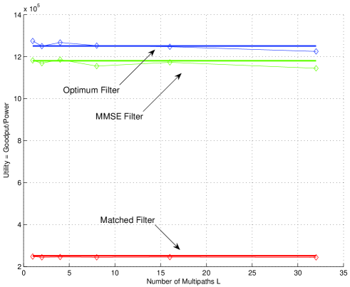
Figure 1: Comparison of theoretic values and simulations for utilities in the Nash equilibrium.

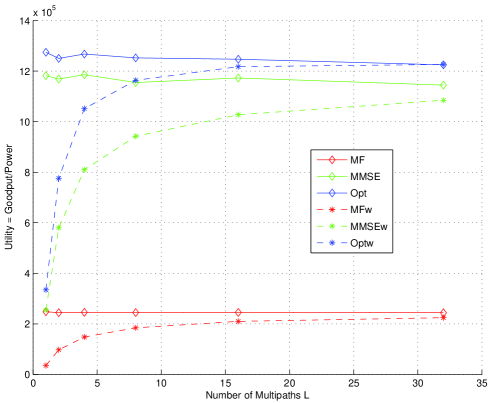
Figure 2: Simulation of utilities in the Nash equilibrium and constant power allocations versus $L$.

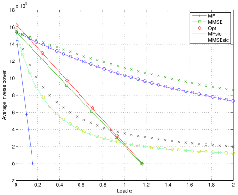
Figure 3: Average inverse power used by the different filters.

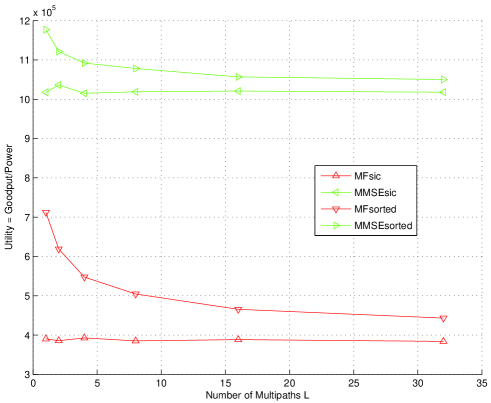
Figure 4: Simulation of utilities in the Nash equilibrium with SIC filter with and without optimal ordering, versus $L$.

X Conclusion

Using tools of random matrices, we have derived the equilibrium power allocation in a game-theoretic framework applied to asymptotic CDMA with cyclic prefix, under frequency-selective fading. Three receivers are considered: matched filter, MMSE and optimum filter (given by Shannon’s capacity). In addition, distributed ordering mechanisms are introduced and the successive interference cancellation variants of the linear filters are studied. For each user, this power allocation depends only on the total energy of the channel of the user under consideration. For a frequency-flat channel, the power allocation among users is dis-uniform, whereas when the number of multipaths increases, the power allocation tends more and more to a uniform one.

XI Appendix

XI-A Proof of Prop. 3

Notice that when $\sigma^{2}\rightarrow\infty$, ${C}^{\textrm{OPT}}=0$, ${C}^{\textrm{MMSE}}=0$ and $\beta^{\textrm{MMSE}}(x)=\beta(x)=0$. Thus we only have to prove that the derivatives of either side of (20) are equal.

Using $\rho(f,x)=P(x)\left\lvert h(f,x)\right\rvert^{2}$, (13) can be rewritten

$$\beta(x)=\int_{0}^{1}\frac{\rho(f,x)df}{\sigma^{2}+\int_{0}^{\alpha}\frac{\rho(f,y)2dy}{1+\beta(y)}}.$$ (49)

From (1), $\int_{0}^{1}\rho(f,x)u(f,-\sigma^{2})df$ satisfies the same implicit equation (49) as $\beta(x)$ and thus

$$u(f,-\sigma^{2})=\frac{1}{\int_{0}^{\alpha}\frac{\rho(f,y)dy}{1+\beta(y)}+\sigma^{2}}.$$ (50)

Using (49) and (50), we can rewrite

$$\int_{0}^{1}u (f,-\sigma^{2})df-\frac{1}{\sigma^{2}}$$

$$=\int_{0}^{1}\frac{1}{\int_{0}^{\alpha}\frac{\rho(f,y)dy}{1+\beta(y)}+\sigma^{2}}df-\int_{0}^{1}\frac{1}{\sigma^{2}}df$$

$$=\int_{0}^{1}\frac{-\int_{0}^{\alpha}\frac{\rho(f,x)}{1+\beta(x)}dx}{\sigma^{2}\left(\int_{0}^{\alpha}\frac{\rho(f,y)dy}{1+\beta(y)}+\sigma^{2}\right)}df$$

$$=\int_{0}^{\alpha}\frac{\frac{-1}{\left(1+\beta(x)\right)}}{\sigma^{2}}\int_{0}^{1}\frac{\rho(f,x)df}{\int_{0}^{\alpha}\frac{\rho(f,y)dy}{1+\beta(y)}+\sigma^{2}}dx$$

$$=-\int_{0}^{\alpha}\frac{\beta(x)}{\sigma^{2}\left(1+\beta(x)\right)}dx.$$

Thus from (18)

$$\frac{\partial{C}^{\textrm{OPT}}}{\partial\sigma^{2}}=-\log_{2}(e)\int_{0}^{\alpha}\frac{\beta(x)}{\sigma^{2}\left(1+\beta(x)\right)}dx.$$ (51)

Differentiating (15) with respect to $\sigma^{2}$, we obtain

$$\frac{\partial{C}^{\textrm{MMSE}}}{\partial\sigma^{2}}=\log_{2}(e)\int_{0}^{\alpha}\frac{1}{1+\beta(x)}\frac{\partial\beta}{\partial{\sigma^{2}}}(x)dx.$$ (52)

Let $\pi(x)=\frac{1}{\sigma^{2}(1+\beta(x))}$. From (51) and (52), we obtain

$$\frac{\partial{C}^{\textrm{OPT}}}{\partial\sigma^{2}}-\frac{\partial{C}^{\textrm{MMSE}}}{\partial\sigma^{2}}\\ =-\log_{2}(e)\int_{0}^{\alpha}\left(\beta(x)+\sigma^{2}\frac{\partial\beta}{\partial{\sigma^{2}}}(x)\right)\pi(x)dx.$$ (53)

From (13), we have

$$\int_{0}^{\alpha}\sigma^{2}\beta(x)\frac{\partial\pi}{\partial\sigma^{2}}(x)dx$$

$$=\int_{0}^{\alpha}\int_{0}^{1}\frac{\sigma^{2}\rho(f,x)df}{\sigma^{2}+\int_{0}^{\alpha}\sigma^{2}\rho(f,y)\pi(y)dy}\frac{\partial\pi}{\partial\sigma^{2}}(x)dx$$

$$=\int_{0}^{1}\frac{\int_{0}^{\alpha}\rho(f,x)\frac{\partial\pi}{\partial\sigma^{2}}(x)dx}{1+\int_{0}^{\alpha}\rho(f,y)\pi(y)dy}df$$

$$=\frac{1}{\log_{2}(e)}\frac{\partial}{\partial\sigma^{2}}\int_{0}^{1}\log_{2}\left(1+\int_{0}^{\alpha}\rho(f,y)\pi(y)dy\right)df.$$

Observing that

$$\int_{0}^{\alpha}\left(\beta(x)+\sigma^{2}\frac{\partial\beta}{\partial{\sigma^{2}}}(x)\right)\pi(x)+\sigma^{2}\beta(x)\frac{\partial\pi}{\partial\sigma^{2}}(x)dx\\ =\frac{\partial}{\partial\sigma^{2}}\int_{0}^{\alpha}\sigma^{2}\beta(x)\pi(x)dx$$

we obtain (20) from Prop. 3.

XI-B Influence of Other Players’ Strategies

We want to prove that asymptotically, in the game $\{S^{K},{\mathbb{P}},(u_{k})_{k\in S^{K}}\}$, the strategy of a single player does not have any influence on the payoff of the other players. In other words, for all $k\neq i\in S^{K}$, for all ${\bf p}=(P_{1},\dotsc,P_{K})\in{\mathbb{P}}^{K}$, for all $P^{\prime}_{i}\in{\mathbb{P}}$,

$$\left\lvert u_{k}({\bf p})-u_{k}(P^{\prime}_{i},{\bf p}_{(-i)})\right\rvert\to 0,\ \textrm{as}\ N\to\infty.$$

Remember that $u_{k}=\frac{{\gamma}(\beta_{k})}{P_{k}}$, and ${\gamma}$ is at least $C^{2}$. Let $(\beta_{1},\dotsc,\beta_{K})$ be the SINRs associated with the power allocation ${\bf p}$ and $(\beta^{\prime}_{1},\dotsc,\beta^{\prime}_{K})$ the SINRs associated with the power allocation $(P^{\prime}_{i},{\bf p}_{(-i)})$. Then a simple Taylor expansion of ${\gamma}$ in $\beta^{\prime}_{k}$ gives

$${\gamma}(\beta^{\prime}_{k})={\gamma}(\beta_{k})+(\beta^{\prime}_{k}-\beta_{k})\frac{\partial{\gamma}}{\partial\beta}(\beta_{k})+o(\beta^{\prime}_{k}-\beta_{k}).$$ (54)

According to (54), it is sufficient to show that

$$\left\lvert\frac{\beta^{\prime}_{k}-\beta_{k}}{P_{k}}\right\rvert\to 0,\ \textrm{as}\ N\to\infty.$$ (55)

Matched Filter

For the matched filter, the inequality is obtained directly from (11). The denominator of (11) is always greater than $\frac{\sigma^{2}}{N}\sum_{n=1}^{N}\left\lvert{{h}_{{n}{k}}}\right\rvert^{2}$. Hence,

$$\left\lvert\frac{\beta^{\prime}_{k}-\beta_{k}}{P_{k}}\right\rvert \leq\left\lvert\frac{P_{k}\frac{1}{N}(P^{\prime}_{i}-P_{i})\frac{1}{N}\sum_{n=1}^{N}\left\lvert{{h}_{{n}{i}}}\right\rvert^{2}\left\lvert{{h}_{{n}{k}}}\right\rvert^{2}}{P_{k}\sigma^{4}}\right\rvert$$

$$\leq\frac{P_{\text{max}}h_{\text{max}}^{2}}{\sigma^{4}N}.$$

MMSE Filter

For the MMSE filter, the inequality is obtained from (12), Lemma 1 from [33] and Lemma 2.1 from [41], which we both reproduce below for convenience.

Lemma 1

[33] Let ${\bf C}$ be a $N\times N$ complex matrix with uniformely bounded spectral radius for all $N$: $\sup_{N}(\left\lvert{\bf C}\right\rvert)<\infty$. Let ${\bf w}=\frac{1}{\sqrt{N}}[w_{1},\dotsc,w_{N}]^{T}$ where $\{w_{i}\}_{i=1\dotsc N}$ are i.i.d. complex random variables with zero mean, unit variance and finite eighth moment. Then:

$${{\mathbb{E}}\left[\left\lvert{\bf w}^{H}{\bf C}{\bf w}-\frac{1}{N}{\mathrm{tr}}{{\bf C}}\right\rvert^{4}\right]}\leq\frac{C}{N^{2}}$$

where $C$ is a constant that does not depend on $N$ or ${\bf C}$.

Lemma 2

[41] Let $\sigma^{2}>0$, ${\bf A}$ and ${\bf B}$ $N\times N$ with ${\bf B}$ Hermitian nonnegative definite, and ${\bf q}\in{\mathbb{C}}^{N}$. Then

$${\mathrm{tr}}\left(\left(({\bf B}+\sigma^{2}{\bf I})^{-1}-({\bf B}+{\bf q}{\bf q}^{H}+\sigma^{2}{\bf I})^{-1}\right){\bf A}\right)\leq\frac{\left\lVert{\bf A}\right\rVert}{\sigma^{2}}.$$

In Lemma 2, $\left\lVert{\bf A}\right\rVert$ is the spectral norm of ${\bf A}$, i.e., the square root of the largest singular value of ${\bf A}$.

From (7), we can write

$$\beta_{k}=P_{k}{{\bf w}_{k}}^{H}{\bf H}_{k}^{H}\left({{\bf G}}_{(-k)}{{\bf G}}_{(-k)}^{H}+\sigma^{2}{\bf I}_{N}\right)^{-1}{\bf H}_{k}{{\bf w}_{k}},$$

$$\beta^{\prime}_{k}=P_{k}{{\bf w}_{k}}^{H}{\bf H}_{k}^{H}\left({{{\bf G}}_{(-k)}}^{\prime}{{{\bf G}}_{(-k)}^{H}}^{\prime}+\sigma^{2}{\bf I}_{N}\right)^{-1}{\bf H}_{k}{{\bf w}_{k}}$$

where

$${{{\bf G}}_{(-k)}}^{\prime}{{{\bf G}}_{(-k)}^{H}}^{\prime}={{\bf G}}_{(-k)}{{\bf G}}_{(-k)}^{H}\\ +(P^{\prime}_{i}-P_{i})({{\bf h}_{i}}\odot{{\bf w}_{i}})({{\bf h}_{i}}\odot{{\bf w}_{i}})^{H}.$$

A corollary of Lemma 1 is that for either matrix ${\bf C}={\bf H}_{k}^{H}\left({{\bf G}}_{(-k)}{{\bf G}}_{(-k)}^{H}+\sigma^{2}{\bf I}_{N}\right)^{-1}{\bf H}_{k}$ or matrix ${\bf C}={\bf H}_{k}^{H}\left({{{\bf G}}_{(-k)}}^{\prime}{{{\bf G}}_{(-k)}^{H}}^{\prime}+\sigma^{2}{\bf I}_{N}\right)^{-1}{\bf H}_{k}$, we obtain [33]

$$\left\lvert{{\bf w}_{k}}^{H}{\bf C}{{\bf w}_{k}}-\frac{1}{N}{\mathrm{tr}}{{\bf C}}\right\rvert\to 0,\ \textrm{as}\ N\to\infty.$$

Matrix ${\bf B}={{\bf G}}_{(-k)}{{\bf G}}_{(-k)}^{H}$ is Hermitian nonnegative definite, as for all ${\bf w}\in{\mathbb{C}}^{N}$, ${\bf w}^{H}{{\bf G}}_{(-k)}{{\bf G}}_{(-k)}^{H}{\bf w}=\left\lVert{{\bf G}}_{(-k)}{\bf w}\right\rVert^{2}\geq 0$. Diagonal matrix ${\bf A}={\bf H}_{k}{\bf H}_{k}^{H}$ has spectral norm $\left\lVert{\bf H}_{k}{\bf H}_{k}^{H}\right\rVert\leq h_{\text{max}}^{2}$. Using Lemmas 1 and 2, as $N\to\infty$, we obtain

$$\left\lvert\frac{\beta^{\prime}_{k}-\beta_{k}}{P_{k}}\right\rvert\to 0,\ \textrm{as}\ N\to\infty.$$

Optimum and Successive Interference Cancellation Filters

The analog of the SINR derived for the optimum filter stems from the MMSE filter with SIC. The SINR for SIC filters have similar expressions with less interfering users appearing in the denominator. Hence the result is immediate.

XI-C Proof of Prop. 5

Given ${C}^{\star}$, we can use (20) to obtain a Nash equilibrium power allocation in the following way. We rewrite (20) assuming that the target SINR for the MMSE filter is $\beta^{+}$.

$$\alpha\log_{2}\left(1+\beta^{+}\right)-\alpha\log_{2}(e)\frac{\beta^{+}}{1+\beta^{+}}\\ +\log_{2}\left(1+\frac{1}{\sigma^{2}\left(1+\beta^{+}\right)}\int_{0}^{\alpha}P(y)\left\lvert h(y)\right\rvert^{2}dy\right)\\ =\alpha\log_{2}\left(1+\beta^{\star}\right).$$ (56)

In the left-hand side of (56), $P(y)$ is given by a MMSE power allocation similar to the one given by (28). Hence, the term $\int_{0}^{\alpha}P(y)\left\lvert h(y)\right\rvert^{2}dy$ in (56) does not depend on the actual realizations of the channels. Replacing $\beta^{\star}$ by $\beta^{+}$ in (27), we obtain that $\int_{0}^{\alpha}P(y)\left\lvert h(y)\right\rvert^{2}dy=\frac{\alpha\sigma^{2}\beta^{+}}{1-\alpha\frac{\beta^{+}}{1+\beta^{+}}}$, which gives us (30). Replacing $\beta^{\star}$ by $\beta^{+}$ in (28), we obtain the power allocation (29).

XI-D Expectation of the random variable (33)

For each user $j$, there are $L>1$ paths with respective attenuations $h_{\ell}\left(\frac{j}{N}\right),\ \ell=1,\dotsc,L$, which are i.i.d. complex random variables with mean zero and even distributions of the real and imaginary parts. The Fourier transform of those attenuations is ${{h}_{{n}{j}}}=h\left(\frac{n}{N},\frac{j}{N}\right)=\sum_{\ell=1}^{L}h_{\ell}\left(\frac{j}{N}\right)e^{-2\pi i\frac{n}{N}(\ell-1)}$. The total energy of the paths is $E_{j}=\sum_{\ell=1}^{L}\left\lvert h_{\ell}\left(\frac{j}{N}\right)\right\rvert^{2}$.

We want to show that the expectation of the random variable $\frac{1}{K}\sum_{j=1}^{K}\frac{\left\lvert{{h}_{{n}{j}}}\right\rvert^{2}}{E_{j}}$ is equal to 1. By expanding the expression of ${{h}_{{n}{j}}}$, this is equivalent to showing that the expectation of the random variable

$$\frac{h_{\ell}\left(\frac{j}{N}\right)h_{\ell^{\prime}}\left(\frac{j^{\prime}}{N}\right)}{E_{j}}$$

is equal to 0. Denoting by $p(\cdot)$ the distribution of $h_{\ell}=h_{\ell}\left(\frac{j}{N}\right)$, this expectation is equal to the $L$-dimensional integral of

$$\frac{h_{\ell}h_{\ell^{\prime}}}{\left\lvert h_{\ell}\right\rvert^{2}+\left\lvert h_{\ell^{\prime}}\right\rvert^{2}+\sum_{k\neq\ell,\ell^{\prime}}\left\lvert h_{k}\right\rvert^{2}}p\left(h_{\ell}\right)p\left(h_{\ell^{\prime}}\right)\prod_{k\neq\ell,\ell^{\prime}}p\left(h_{k}\right)$$

which is an odd function of $h_{\ell}$. Its integral is therefore 0, which proves the desired result.

XI-E Proof of (45) and (46)

Denote $m_{k}=P_{K-k}\left\lvert h_{K-k}\right\rvert$. From (42), with flat fading, the sequence $\{m_{k}\}_{k\in S^{K}}$ satisfies $m_{0}=\beta^{\star}\sigma^{2}$ and $m_{k+1}=\beta^{\star}\sigma^{2}+\frac{\beta^{\star}}{N}\sum_{j=0}^{k}m_{j}$. Using the fact that $\sum_{i=j}^{k}\binom{i}{j}=\binom{k+1}{j+1}$, it is immediate to prove by recurrence that

$$m_{k}=\beta^{\star}\sigma^{2}\sum_{j=0}^{k}\binom{k}{j}\frac{1}{N^{j}}{\beta^{\star}}^{j}=\beta^{\star}\sigma^{2}\left(1+\frac{1}{N}\beta^{\star}\right)^{k}.$$

Hence formula (45). The demonstration is exactly similar for (46) from the recursion $m_{0}=\beta^{\star}\sigma^{2}$ and $m_{k+1}=\beta^{\star}\sigma^{2}+\frac{\beta^{\star}}{\left(1+\beta^{\star}\right)N}\sum_{j=0}^{k}m_{j}$.

XI-F Optimal Ordering of Users

We determine the ordering that makes use of the least total power for equilibrium PA (45) (the case is similar for (46), (47) and (48)). Let the ordering of the users be such as $\left\lvert h_{1}\right\rvert^{2}<\dotsb<\left\lvert h_{K}\right\rvert^{2}$. Let $\pi$ be any permutation of $\{1,\dotsc,K\}$. Let $a_{ij}=\left(1+\frac{1}{N}\beta^{\star}\right)^{K-i}-\left(1+\frac{1}{N}\beta^{\star}\right)^{K-j}$.

Then showing that the optimal ordering is such as $\left\lvert h_{1}\right\rvert^{2}<\dotsb<\left\lvert h_{K}\right\rvert^{2}$ is equivalent to showing that for any $\pi$

$$\sum_{k=1}^{K}\frac{1}{\left\lvert h_{k}\right\rvert^{2}}a_{k\pi(k)}>0.$$ (57)

Consider first a cyclic permutation. By the definition of $a_{ij}$, the sum of the $a_{k\pi(k)}$ is equal to zero: $\sum_{k=1}^{K}a_{k\pi(k)}=0$. The first coefficient $a_{1\pi(1)}$ is positive. It is affected coefficient $\frac{1}{\left\lvert h_{1}\right\rvert^{2}}$, which is the greatest coefficient in the sum in (57). Hence the sum in (57) is positive in this case.

Permutation $\pi$ can be decomposed as a product of disjoint permutation cycles. Each cycle determines a subset of indexes $k$, these subsets form a partition of $\{1,\dotsc,K\}$. With a similar reasoning as precedently, replacing index $1$ with the smallest index in the cycle, the sum over the indexes $k$ pertaining to a cycle of $\frac{1}{\left\lvert h_{k}\right\rvert^{2}}a_{k\pi(k)}$ is positive. Hence the global sum of (57) is also positive.

It can be proven in a similar way that the same ordering maximizes the sum of inverse powers of the users.

XII Acknowledgements

The authors would like to thank Prof. J. Silverstein for pointing us to reference [41].

References

• [1] J. Zander, “Performance of Optimum Transmitter Power Control in Cellular Radio Systems,” IEEE Trans. on Veh. Technol., vol. 41, no. 1, pp. 57–62, Feb. 1992.
• [2] S. Grandhi, R. Vijayan, D. Goodman, and J. Zander, “Centralized Power Control in Cellular Radio Systems,” IEEE Trans. on Veh. Technol., vol. 42, no. 4, pp. 466–468, Nov. 1993.
• [3] Q. Wu, “Performance of Optimal Transmitter Power Control in CDMA Cellular Mobile Systems,” IEEE Trans. on Veh. Technol., vol. 48, no. 2, pp. 571–575, Mar. 1999.
• [4] D. Tse and S. Hanly, “Multiaccess Fading Channel–Part I: Polymatroid Structure, Optimal Resource Allocation and Throughput Capacity,” IEEE Trans. on Information Theory, vol. 44, no. 7, pp. 2796–2815, Nov. 1998.
• [5] A. El-Osery and C. Abdallah, “Distributed Power Control in CDMA Cellular Systems,” IEEE Trans. on Antennas and Propagation, vol. 42, no. 4, pp. 152–159, Aug. 2000.
• [6] G. J. Foschini and Z. Miljanic, “A Simple Distributed Autonomous Power Control Algorithm and its Convergence,” IEEE Trans. on Veh. Technol., vol. 42, no. 4, pp. 641–646, Nov. 1993.
• [7] S. Grandhi, R. Vijayan, and D. Goodman, “Distributed Power Control in Cellular Radio Systems,” IEEE Trans. on Communications, vol. 42, no. 2/3/4, pp. 226–228, February/March/April 1994.
• [8] R. Yates, “A Framework for Uplink Power Control in Cellular Radio Systems,” IEEE Journal on Selected Areas in Communications, vol. 13, no. 7, pp. 1341–1347, Sept. 1995.
• [9] E. Altman, T. Boulogne, R. E. Azouzi, T. Jimenez, and L. Wynter, “A survey on networking games,” Computers and Operations Research, 2006.
• [10] D. Goodman and N. Mandayam, “Power Control for Wireless Data,” IEEE Personal Communications, vol. 7, no. 2, pp. 48–54, 2000.
• [11] A. MacKenzie and S. Wicker, “Game Theory and the Design of Self-Configuring, Adaptive Wireless Networks,” IEEE Trans. on Communications, Nov. 2001.
• [12] A. Tulino and S. Verdú, “Random matrix theory and wireless communications,” Foundations and Trends in Communications and Information Theory, vol. 1, no. 1, 2004.
• [13] S. Verdú and S. Shamai, “Spectral Efficiency of CDMA with Random Spreading ,” IEEE Trans. on Information Theory, pp. 622–640, Mar. 1999.
• [14] D. Tse and S. Hanly, “Linear Multiuser Receivers: Effective Interference, Effective Bandwidth and User Capacity,” IEEE Trans. on Information Theory, vol. 45, no. 2, pp. 641–657, Mar. 1999.
• [15] S. Shamai and S. Verdú, “The Effect of Frequency-Flat Fading on the Spectral Efficiency of CDMA,” IEEE Trans. on Information Theory, vol. 47, no. 4, pp. 1302–1327, May 2001.
• [16] A. Tulino, L. Li, and S. Verdú, “Spectral Efficiency of Multicarrier CDMA,” IEEE Trans. on Information Theory, vol. 51, no. 2, pp. 479–505, February 2005.
• [17] J. Wardrop, “Some Theoretical Aspects of Road Traffic Research Communication Networks,” in Proc. Inst. Civ. Eng., vol. 2, no. 1, 1952, pp. 325–378.
• [18] A. Haurie and P. Marcotte, “On the Relationship between Nash-Cournot and Wardrop Equilibria,” Networks, vol. 15, pp. 295–308, 1985.
• [19] R. Müller and S. Verdú, “Design and Analysis of Low-Complexity Interference Mitigation on Vector Channels,” IEEE Journal on Selected Areas in Communications, pp. 1429–1441, Aug. 2001.
• [20] B. M. Hochwald, T. L. Marzetta, and V. Tarokh, “Multiple-Antenna Channel Hardening and Its Implications for Rate Feedback and Scheduling,” IEEE Trans. on Information Theory, vol. 50, no. 9, pp. 1893–1909, Sept. 2004.
• [21] V. Rodriguez, “Robust Modeling and Analysis for Wireless Data Resource Management,” in Proceedings of the IEEE Wireless Communications & Networking Conference, Mar. 2003.
• [22] H. Ji, “Resource Management in Communication Networks via Economic Models,” Ph.D. dissertation, Rutgers University, New Jersey, 1997.
• [23] C. Saraydar, N. Mandayam, and D. Goodman, “Efficient Power Control via Pricing in Wireless Data Networks,” IEEE Trans. on Communications, vol. 50, no. 2, pp. 291–303, Feb. 2002.
• [24] F. Meshkati, H. Poor, S. Schwartz, and N. Mandayam, “An Energy-Efficient Approach to Power Control and Receiver Design in Wireless Data Networks,” IEEE Trans. on Communications, vol. 53, no. 11, pp. 1885–1894, Nov. 2005.
• [25] F. Meshkati, M. Chiang, H. Poor, and S. Schwartz, “A Game-Theoretic Approach to Energy-Efficient Power Control in Multi-Carrier CDMA Systems,” IEEE Journal on Selected Areas in Communications, 2006.
• [26] V. Girko, Theory of Random Determinants.   Kluwer Academic Publishers, Dordrecht, The Netherlands, 1990.
• [27] J. Silverstein and Z. Bai, “On the Empirical Distribution of Eigenvalues of a Class of Large Dimensional Random Matrices,” J. Multivariate Anal., vol. 54, no. 2, pp. 175–192, 1995.
• [28] N. Bonneau, M. Debbah, E. Altman, and A. Hjørungnes, “Wardrop Equilibrium for CDMA Systems,” in Rawnet 2007, Limassol, Cyprus, Apr. 2007.
• [29] R. Gray, “Toeplitz and Circulant Matrices: A Review,” Foundations and Trends in Communications and Information Theory, vol. 2, no. 3, pp. 155–239, 2006.
• [30] K. Fazel and L. Papke, “On the Performance of Convolutionally-Coded CDMA/OFDM for Mobile Communication System,” in Proceedings of IEEE PIMRC, Yokohama, Japan, Sept. 1993, pp. 468–472.
• [31] J. Lindner, “MC-CDMA and its Relation to General Multiuser/Multisubchannel Transmission Systems,” in International Symposium on Spread Spectrum Techniques & Applications, Mainz, Germany, Sept. 1996, pp. 115–121.
• [32] J. Bingham, “Multicarrier Modulation for Data Transmission: An Idea Whose Time Has Come,” IEEE Communications Magazine, vol. 28, no. 5, pp. 5–14, May 1990.
• [33] J. Evans and D. Tse, “Large System Performance of Linear Multiuser Receivers in Multipath Fading Channels,” IEEE Trans. on Information Theory, pp. 2059–2078, Sept. 2000.
• [34] W. Hachem, “Simple Polynomial Detectors for CDMA Downlink Transmissions on Frequency-Selective Channels,” IEEE Trans. on Information Theory, vol. 50, no. 1, pp. 164–171, January 2004.
• [35] R. Müller, “Multiuser Receivers for Randomly Spread Signals: Fundamental Limits with and without Decision-Feedback,” IEEE Trans. on Information Theory, vol. 47, no. 1, pp. 268–283, Jan. 2001.
• [36] R. Aumann, “Subjectivity and Correlation in Randomized Strategies,” Journal of Mathematical Economics, vol. 1, pp. 67–96, 1974.
• [37] ——, “Correlated Equilibrium as an Expression of Bayesian Rationality,” Journal of Mathematical Economics, vol. 55, pp. 1–18, 1987.
• [38] S. Hart and D. Schmeidler, “Existence of Correlated Equilibria,” Mathematics of Operations Research, vol. 14, no. 1, pp. 18–25, Feb. 1989.
• [39] A. Neyman, “Correlated Equilibrium and Potential Games,” International Journal of Game Theory, vol. 26, pp. 223–227, 1997.
• [40] E. Altman, N. Bonneau, and M. Debbah, “Correlated Equilibrium in Access Control for Wireless Communications,” in Networking 2006, Coimbra, Portugal, May 2006.
• [41] Z. Bai and J. Silverstein, “On the Signal-to-Interference Ratio of CDMA Systems in Wireless Communications,” Annals of Probability, vol. 17, no. 1, pp. 81–101, 2007.