Self force of a static electric charge near a Schwarzschild Star

Abstract

When a charge is held static near a constant density spherical star, it experiences a self-force $\mathrm{F}_{\mathrm{self}}$, which is significantly different from the force $\mathrm{F}_{\mathrm{self}}^{\mathrm{BH}}$ it would experience when placed near a black hole of the same mass. In this paper, an expression for the self-force (as measured by a locally inertial observer) is given for an insulating Schwarzschild star, and the result is explicitly computed for the extreme density case, which has a singularity at its center. The force is found to be repulsive. A similar calculation of the self-force is also performed for a conducting star. This calculation is valid for any static, spherically conducting star, since the result is independent of the interior metric. When the charge is placed very close to the conducting star, the force is found to be attractive but when the charge is placed beyond a certain distance (2.95M for a conducting star of radius 2.25M), the force is found to be repulsive. When the charge is placed very far from the star (be it conducting or insulating), the charge experiences the same repulsive force it would experience when placed in the spacetime of a black hole with the same mass as the star.

I Introduction

The electrostatic potential and the fields produced by a static electric charge in the vicinity of a Schwarzschild black hole have been discussed in detail in several papers copson ; linet ; wald ; hanni . These all suppose that an external force holds an electric charge $e$ at rest at a coordinate position $R=b$ in the Schwarzschild geometry. This external force should balance the electrostatic force on the charge in addition to the usual attractive gravitational force (on the mass carrying the charge). When there is no other charge anywhere, the entire electrostatic force on the charge may be regarded as a self-force.

An explicit expression for the electrostatic potential of such a point charge is given as a summation over multipole moments in wald . The horizon of the black hole is found to be an equipotential surface and hanni shows the electric lines of force everywhere outside the horizon. A closed form expression for a specific potential, $V^{\rm C}$, was given earlier by Copson copson , using work of Hadamard hadamard , but it corresponds to a solution with non-zero charge on the black hole. For the potential corresponding to physically relevant boundary conditions (namely, zero net charge on the black hole), Linetlinet observed that a spherically symmetric homogeneous solution had to be added to Copson’s potential, yielding a result in accord with wald .

By employing a strategy similar to Dirac’sdirac , of imposing conservation of the stress energy tensor inside a world-tube surrounding the particle and then limiting the world tube to the world line of the particle, Smith and WillWill calculated the external force needed to hold this charge at rest. After subtracting the requisite gravitational force, the electrostatic self-force is found to be $F_{\mathrm{self}}^{\mathrm{BH}}=e^{2}M/b^{3}$. It is implicit that this force is always calculated with respect to a locally inertial observer at the position of the charge. The potential of wald or linet is essential for understanding this result: with the potential, $V^{\rm C}$, given by Copsoncopson , no self-force would have been found.

A static electric charge is a singular point source and the potentials discussed so far all satisfy Maxwell’s equations with the point particle as source. This is quite distinct from the behavior of the so-called “direct” and “tail” fields dewitt:brehme , for which the source in Maxwell’s equations is not well identified. By contrast, the radiation potential of Diracdirac satisfies Maxwell’s equations with no source. Other familiar potentials which satisfy Maxwell’s equations with the point particle as source include the retarded and advanced potentials, and their symmetric sum. Ironically, Copson’s potential in copson is none of these familiar constructs, nor is the potential of wald ; linet .

Detweiler and Whitingbernard demonstrate that, in general, a potential $V$ due to a point source can be written as sum of two parts, $V=V^{\rm S}+V^{\rm R}$, where $V^{\rm S}$ is a singular potential (divergent at the particle) which exerts no self force on the particle and $V^{\rm R}$ is the regular potential which is entirely responsible for the self-force. In particular, locally near the source, $V^{\rm S}$ satisfies Maxwell’s equations with the point particle as source, while $V^{\rm R}$ is an homogeneous solution, without source. Within a normal neighborhood of the point charge, the singular potential can be obtained from a variant of Hadamard’s form of the Green’s functionhadamard . We will need to understand its relation to the potential, $V^{\rm C}$, of Copson, that is, locally.

I.1 The Singular Potential

It can be understood that Copson’s potential for this static problem is exactly $V^{\rm S}$ because of the relation between the construction of $V^{\rm S}$ in bernard and Copson’s construction of $V^{\rm C}$ using Hadamard’s work. In constructing the potential we refer to as $V^{\rm C}$, Copson used the unique, locally-represented, least-singular (hence) elementary solution for the static problem, as given in a general formalism due to Hadamardhadamard . By construction, the singularity in $V^{\rm C}$ at the source is of as low an order as is possible. In the not necessarily static case, the singular potential $V^{S}$ is, in a normal neighborhood of the point charge, the unique locally-determined, similarly least-singular solution of generalized Hadamard formbernard , which has support on and outside the light-cone (it exerts no force). In this regard, $V^{\rm S}$ is unique, due to its lack of (local) support inside the light cones. In the static case, when the light-cone collapses and time derivatives disappear in the equation for the potential, the domain of support for $V^{S}$ becomes precisely the domain in which $V^{\rm C}$ is defined. Then, $V^{\rm C}$ and $V^{\rm S}$ solve the same problem under the same conditions, and hence coincide.

The result that Copson’s potential $V^{\rm C}$ is precisely $V^{\rm S}$, is indeed compatible with the fact that it yields no self-force. Consequently, the correction to Copson’s potential given in linet automatically corresponds to $V^{\rm R}$, the regular part of the potential, which provides the self force.

I.2 Overview

In this paper, we consider replacing the black hole by a constant density star. The fundamental fact we will use is that, locally, the potential constructed by Copson $V^{\rm C}$ is exactly the singular piece $V^{\rm S}$, as long as the metric in the neighbourhood of the charge is the Schwarzschild metric. Any additional part of the potential at the position of the charge will contribute to the self force. Our aim is to calculate the self force of a charge $e$ placed in the vicinity of a spherical star in two different situations — depending upon whether the star is totally conducting or totally insulating. Since the metric outside the star is the Schwarzschild metric, Copson’s potential is indeed $V^{\rm S}$. To calculate the self force, we follow Linetlinet by first finding the homogenous solution of Maxwell’s equations $\widetilde{V}$, which should be added to $V^{\rm S}$ (given by Copson) to give the whole potential.

In section II, we briefly discuss the Schwarzschild black hole metric, and the metric of a constant density (Schwarzschild) star, which we show is conformally related to a much simpler metric. In section III, we obtain the solutions to Maxwell’s equations inside and outside the star. We start with the singular potential $V^{\rm S}$ outside the star and continue the solution inside the star’s surface. This reveals that the surface of the star carries a charge distribution, a result which is not physically acceptable. We correct this in section 4, where we impose two different, physically interesting, boundary conditions to calculate the homogeneous solution $\widetilde{V}$, which in turn is responsible for the self force. In section IV.1, we consider an insulating star that does not get electrically polarized. An additional, regular field, arising both inside and outside the star, is necessary to cancel the surface charge induced by $V^{\rm S}$. It is this additional field which is responsible for the self force on the particle. We find that the self force $F_{\mathrm{self}}$, is repulsive and is significantly different from $F_{\mathrm{self}}^{\mathrm{BH}}$ when the charge is placed very close to the star. In section IV.2, we consider a conducting star which has no electric field in the interior, but nevertheless requires an additional field in the exterior to remove the net surface charge which would otherwise be induced on the star. Here, we find that $F_{\mathrm{self}}$ is attractive when the charge is placed close to the star ($b<2.95M$) and is repulsive when the charge is placed farther than $2.95M$. We should interpret the attractive force as a consequence of electrical polarization of the star and the repulsive force as due to interaction of the fields with space-time curvature.

I.3 Discussion

For calculating the self force of a point source in curved spacetime, a variety of regularization techniques have been useddewitt:brehme ; barack:ori ; quinn:wald ; bernard . In a case somewhat related to ours, with a point source placed near a thin shell, Burko et al.burko:etal have explicitly shown how the regularization techniques can be used to calculate the self force. In this paper, we do not perform a regularization to calculate the self force, but we very much rely on the regularization details in Will ; bernard .

We have focused on the extreme density case because of its intrinsic interest. In principle, our approach here can be used to calculate the self-force on a static electric charge in the vicinity of any star with a spherically symmetric metric, not just a star with constant density. Generally, the resulting expression for the self-force would be very complicated and would require numerical evaluation, which is actually what we resort to in the final step of evaluation of the self-force in this paper. It would be interesting to investigate whether such results could have any detectable effect on neutron star physics and observations.

Another question that might come to mind is whether the self-force calculated for the static charge $F_{\mathrm{self}}$, has any connection with the self force experienced by a freely falling charge on which no external force acts. DeWitt and DeWitt dewitt have shown that the self force on a moving charge consists of two parts, a radiative part, which removes the energy from the particle and dumps it into the fields and a conservative part, which pushes the particle off a geodesic without removing energy from it. For a slow moving charge, they explicitly show that the conservative part of the self-force is independent of the particle’s velocity. In the context of the charge placed near a black hole, Wisemanwiseman clearly points out that, the self force $F_{\mathrm{self}}^{\mathrm{BH}}$ experienced by the static charge (as calculated by Will and Smith) exactly corresponds to the conservative part of the self-force experienced by a freely falling charge. It is straightforward to see that we can adopt the same interpretation for the self-force calculated in this paper.

II The Metric

Consider a constant density star of total mass $M$ and radius $R_{s}$. The metric outside the surface of the star is the Schwarzschild black hole metric (see, for example, MTW ):

$$ds^{2}=-(1-2M/R)\,dT^{\,2}+\frac{dR^{2}}{(1-2M/R)}+R^{2}d\Omega^{2},\qquad R>R_{s},$$ (1)

and the metric inside the (Schwarzschild) star (see also MTW ) is

$$ds^{2}=-\left[a-\frac{1}{2}\sqrt{1-\alpha R^{2}}\right]^{2}dT^{\,2}+\frac{dR^{2}}{[1-\alpha R^{2}]}+R^{2}d\Omega^{2},\qquad R<R_{s},$$ (2)

where $a=\frac{3}{2}\sqrt{1-2M/R_{s}}$ and $\alpha=2M/R_{s}^{3}$. The quantity $M/R_{s}$ is bounded above by $4/9$. Hence the range of $a$ is also restricted:

$$0<M/R_{s}\leq 4/9\quad\Rightarrow\quad 3/2>a\geq 1/2.$$ (3)

For the extreme density case, when $M/R_{s}=4/9$, we have $a=1/2$ and the center, $R=0$, develops a singularity (the component, $G_{RR}$, of the Einstein tensor blows up).

The Weyl tensor for the metric in (2) evaluates to zero, which means that the metric is conformally flat. This interior metric can be written in the following simpler form:

$$ds^{2}=\frac{4}{\left(1+\alpha r^{2}\right)^{2}}\left[-(\beta^{2}+\alpha r^{2})^{2}\,dt^{2}+dr^{2}+r^{2}d\Omega^{2}\right],$$ (4)

where $\beta^{2}=(2a-1)/(2a+1)$ and the new coordinates are defined as:

$$t=T(2a+1)/4,\quad{\rm and}\quad r=R/(1+\sqrt{1-\alpha R^{2}}).$$ (5)

The coordinate $r$ is a monotonic function of $R$, and $r$ ranges from $0$ to some maximum value, $r_{s}$ at the surface of the star. We have the following expressions for $r_{s}$ and $\beta^{2}$:

$$r_{s}=\frac{R_{s}}{1+\sqrt{1-\frac{2M}{R_{s}}}},\qquad\beta^{2}=\frac{1-2\alpha r_{s}^{2}}{1-\alpha r_{s}^{2}}.$$ (6)

For each constant density star, $\beta^{2}$ is a constant, and it can take values which range between $0$ and ${1}/{2}$. For the extreme density case, we have $\beta=0$, and $r_{s}={3R_{s}}/{4}={27M}/{16}$, in which case the interior metric takes the following form:

$$ds^{2}=\frac{4}{\left(1+\alpha r^{2}\right)^{2}}\left[-\alpha^{2}r^{4}\,dt^{2}+dr^{2}+r^{2}d\Omega^{2}\right].$$ (7)

There exist coordinate transformations which make (4) manifestly conformally flatconf:cords . Except possibly for $\beta=0$, those coordinate transformations mix the spatial and temporal coordinates. Our focus is restricted to electrostatics in this paper. Since Maxwell’s equations are conformally invariant, it will be sufficient to work with the conformal metric evident in (4), obtained by ignoring the conformal factor $4/\left(1+\alpha r^{2}\right)^{2}$. Thus we will use the metric:

$$d\tilde{s}^{2}=\left[-(\beta^{2}+\alpha r^{2})^{2}\,dt^{2}+dr^{2}+r^{2}d\Omega^{2}\right],$$ (8)

when solving for the electrostatic potential in the following section.

III Electrostatics

Maxwell’s equations, which govern the theory of electrodynamics, can be written as

$$\nabla_{\mu}F^{\mu\nu}=4\pi J^{\nu},$$ (9)

where $F_{\mu\nu}=\partial_{\mu}A_{\nu}-\partial_{\nu}A_{\mu}$. In terms of the coordinate derivatives, they can be presented in the following explicit form:

$$\partial_{\mu}(\sqrt{-g}g^{\mu\rho}g^{\nu\sigma}F_{\rho\sigma})=4\pi\sqrt{-g}\,J^{\nu}.$$ (10)

It is evident that Maxwell’s equations are conformally invariant: $F_{\mu\nu}$ remains invariant under a conformal transformation of the metric provided the source term in (10) is defined so that it, too, is invariant under such a transformation. For electrostatics in a static geometry, Maxwell’s equations in the Lorentz gauge ($\nabla_{\mu}A^{\mu}=0$) can be reduced to a single equation:

$$\partial_{i}(\sqrt{-g}g^{ij}g^{00}\partial_{j}A_{0})=4\pi\sqrt{-g}\,J^{0}.$$ (11)

In this paper, we consider a charge, $e$, on the $z$-axis at the coordinate position $R=b$, located outside a static, spherical star. The resulting potential $A_{0}$, which henceforth we denote as $V(r,\theta)$, will be axially symmetric about the $z$-axis.

III.1 Outside the star

To find the potential outside the star, we will solve Maxwell’s equations, which have been reduced to the single equation in (11). In a static, spherically symmetric geometry, this takes the form:

$$\partial_{r}(\sqrt{-g}g^{rr}g^{00}\partial_{r}V)+\partial_{\theta}(\sqrt{-g}g^{\theta\theta}g^{00}\partial_{\theta}V)=4\pi\sqrt{-g}\,J^{0},$$ (12)

where

$$2\pi\sqrt{-g}J^{0} =e\delta(R-b)\delta(\theta)=e\delta(R-b)\,\sin\theta\delta(1-\cos\theta)$$ (13)

$$=e\delta(R-b)\,\sin\theta{\sum_{\ell}\left[(l+\frac{1}{2})P_{\ell}(\cos\theta)\right]}.$$

Using the metric in (1), equation (12) can be written as

$$-\sin\theta\left[\frac{\partial}{\partial R}\left(R^{2}\frac{\partial V}{\partial R}\right)+\frac{1}{(1-2M/R)}\frac{1}{\sin\theta}\frac{\partial}{\partial\theta}\left(\sin\theta\frac{\partial V}{\partial\theta}\right)\right]$$

$$=2e\delta(R-b)\,\sin\theta{\sum_{\ell}{{(\ell+\frac{1}{2})P_{\ell}(\cos\theta)}}}.$$ (14)

We can decompose the solution in terms of Legendre functions as

$$V(R,\theta)=\sum_{\ell}\left[V_{\ell}(R)P_{\ell}(\cos\theta)\right],$$ (15)

and hence simplify (14) to get

$$-\frac{\partial}{\partial R}\left(R^{2}\frac{\partial V_{\ell}}{\partial R}\right)+\frac{\ell(\ell+1)V_{\ell}}{(1-2M/R)}=e(2\ell+1)\delta(R-b).$$ (16)

Copsoncopson constructed a particular solution, $V^{\rm C}(R,\theta)$, to these equations directly from Hadamard’s elementary solutionhadamard . Even though the solution he constructed was in the context of the charge in the presence of a Schwarzschild black hole, his solution will still be a particular solution for the case where the black hole is replaced by a spherical star, because the exterior metric of the spherical star is the same as the black hole metric. Copson gives

$$V^{\rm C}(R,\theta)=\frac{e}{bR}\frac{(b-M)(R-M)-M^{2}\cos\theta}{\sqrt{(R-M)^{2}-2(R-M)(b-M)\cos\theta+(b-M)^{2}-M^{2}\sin^{2}\theta}}.$$ (17)

A calculation similar to that in Will explicitly shows that this potential does not contribute to the electrostatic self force. It has been known for some time bernard that the field produced by any point source can be decomposed into two pieces, a locally-determined, singular field which does not affect the particle’s state of motion and a regular field (which is a solution to the homogeneous field equations in the neighbourhood of the particle) that does; that is, $V=V^{\rm S}+V^{\rm R}$. The singular potential $V^{\rm S}$ has nothing to do with the self-force. It is the regular potential $V^{\rm R}$ which is entirely responsible for the self-force. It was explained in the introduction that $V^{\rm S}(R,\theta)=V^{\rm C}(R,\theta)$.

The singular field $V^{\rm S}$ is an entirely local construct. The boundary conditions and external sources play a part only in determining the regular field $V^{\rm R}$. The regular field interacts with the source and makes it experience a force. It is crucial in determining the path the charge actually follows. The external field (due to other sources) is in general a part of the regular field. Thus, the force experienced by the point charge is a sum of the force due to external field and the self-force. In the absence of any external sources, the force due to the regular field alone corresponds entirely to the self-force.

We can decompose the singular potential (17) in terms of Legendre functions as in (15): $V^{\rm S}(R,\theta)=\sum_{\ell}\left[V_{\ell}^{\rm S}(R)P_{\ell}(\cos\theta)\right]$. Using the results of wald , the multipole moments corresponding to this potential are given by:

$$V_{\ell}^{\rm S}(R)=e\left\{\begin{array}[]{cc}g_{\ell}(b)f_{\ell}(R)-\frac{M}{Rb}\delta_{\ell,0}&\text{for }R>b>R_{s}\\ \vbox{\vskip 14.45377pt}f_{\ell}(b)g_{\ell}(R)-\frac{M}{Rb}\delta_{\ell,0}&\text{for }R_{s}<R<b\\ \end{array}\right.$$ (18)

where

$$f_{\ell}(R)=-\frac{(2\ell+1)!}{2^{\ell}(\ell+1)!\,\ell!\,M^{\ell+1}}(R-2M)\frac{d}{dR}Q_{\ell}(\frac{R}{M}-1),\quad{\rm and}$$ (19)

$$g_{\ell}(R)=\left\{\begin{array}[]{cc}\frac{2^{\ell}\ell!(\ell-1)!M^{\ell}}{(2\ell)!}(R-2M)\frac{d}{dR}P_{\ell}(\frac{R}{M}-1)&\text{for }\ell\neq 0\\ 1&\text{for }\ell=0\\ \end{array}\right.$$ (20)

are the two linearly independent homogeneous solutions to (16). Note the $\ell\!=\!0$ results: $f_{0}(R)\!=\!1/R$ and $g_{0}(R)\!=\!1$. Otherwise, as $R\!\rightarrow\!\infty$, $f_{\ell}(R)\!\rightarrow\!1/R^{(\ell+1)}$ and $g_{\ell}(R)\!\rightarrow\!1\!\times\!R^{\ell}$.

In the next section, we will calculate the regular field $V^{\rm R}$ that should be added to the singular field $V^{\rm S}$ in the vicinity of the charge, so as to satisfy the appropriate boundary conditions. Before that, we solve for the continuation of $V^{\rm S}$ inside the spherical star.

III.2 Inside the star

We assume throughout that the spherical star has a constant density as discussed in section II. Since Maxwell’s equations in four dimensions are conformally invariant (as long as the source is conformally invariant), the solution inside the star can be obtained by using a conformally related metric and a conformally invariant source in Maxwell’s equations. Thus, we will use the conformal metric, (8), when we solve Maxwell’s equations inside the star. The interior potential $V(r,\theta)$, can be found from Maxwell’s equations by using the interior metric (8) in (12):

$$-\sin\theta\left[\frac{\partial}{\partial r}\left(\frac{r^{2}}{(\beta^{2}+\alpha r^{2})}\frac{\partial V}{\partial r}\right)+\frac{1}{(\beta^{2}+\alpha r^{2})}\frac{1}{\sin\theta}\frac{\partial}{\partial\theta}\left(\sin\theta\frac{\partial V}{\partial\theta}\right)\right]=4\pi J^{0}\sqrt{-g}.$$ (21)

We assume that there is no charge inside the surface of the star. Then, $J^{0}\sqrt{-g}$ is the charge density on the star, which can be expressed as $\sigma(\theta)\sin\theta\delta(r-r_{s})$, where $\sigma(\theta)$ is the surface charge density.

By axial symmetry, we can decompose the solution as $V(r,\theta)=\sum_{\ell}V_{\ell}(r)P_{\ell}(\cos\theta)$. We can also decompose the charge density as $\sigma(\theta)=\Sigma_{\ell}\sigma^{\ell}P_{\ell}(\cos\theta)$. Now, (21) reduces to

$$\left[-\frac{\partial}{\partial r}\left(\frac{r^{2}}{(\beta^{2}+\alpha r^{2})}\frac{\partial V_{\ell}}{\partial r}\right)+\frac{\ell(\ell+1)}{(\beta^{2}+\alpha r^{2})}V_{\ell}\right]=\sigma^{\ell}\delta(r-r_{s}).$$ (22)

The homogeneous solutions to (22) are obtained in terms of hypergeometric functions $F([a,b],[c],x)$Arfken . For each $\ell$, there are two linearly independent solutions for $V_{\ell}(r)$, namely $h_{\ell}(r)$, $k_{\ell}(r)$:

$$h_{\ell}(r)=\left\{\begin{array}[]{cc}\left(-\frac{r}{\beta^{2}}\right)^{\ell}\left(1+\frac{\alpha}{\beta^{2}}r^{2}\right)^{2}\,F\left(\left[\frac{3}{2},2+\ell\right],\left[\ell+\frac{3}{2}\right],-\frac{\alpha}{\beta^{2}}r^{2}\right)&\text{for }\beta\neq 0\\ \vbox{\vskip 14.45377pt}(\alpha r)^{-\ell}&\text{ for }\beta=0,\end{array}\right.$$ (23)

and

$$k_{\ell}(r)=\left\{\begin{array}[]{cc}\left(-\frac{\beta^{2}}{r}\right)^{\ell+1}\left(1+\frac{\alpha}{\beta^{2}}r^{2}\right)^{2}\,F\left(\left[\frac{3}{2},1-\ell\right],\left[\frac{1}{2}-\ell\right],-\frac{\alpha}{\beta^{2}}r^{2}\right)&\text{for }\beta\neq 0\\ \vbox{\vskip 14.45377pt}(\alpha r)^{\ell+1}&\text{ for }\beta=0.\end{array}\right.$$ (24)

Note that $h_{0}(r)=1$, is a constant. When $\beta\neq 0$, we see that, for small values of $r$, $h_{\ell}(r)\,\sim\,r^{\ell}$ and $k_{\ell}(r)\,\sim\,r^{-\ell-1}$. Since, for $\beta\neq 0$, we want $V_{\ell}$ to be well behaved at the origin, it should take the form of $h_{\ell}{(r)}$. Away from $r=0$, $h_{\ell}{(r)}$ is well behaved in the limit $\beta\rightarrow 0$, so we propose that $V_{\ell}$ should also take the form of $h_{\ell}{(r)}$ for $\beta=0$.

To find the precise form of the potential $V_{\ell}{(r)}$ for $\ell=0$ and $\beta=0$, we impose the requirement that there is no charge at the center of the star $r=0$. To examine the charge at the center of the star at $r=0$, we consider a small spherical Gaussian surface at $r=\epsilon$ around the center. When we integrate the field due to this potential over this small Gaussian surface, the charge inside it is proportional to (see appendix A)

$$\frac{r^{2}}{\beta^{2}+\alpha r^{2}}\frac{dV_{0}(r)}{dr}\bigg{|}_{r=\epsilon}.$$

Only the $\ell=0$ term would survive because the integral would involve a term of $P_{\ell}{(\mathrm{cos\theta})}$ integrated over the surface. Requirement that the charge at the center should vanish implies that for $\beta=0$, the potential $V_{0}{(r)}$ takes the form of $h_{0}{(r)}$ which is a constant. There is no ambiguity.

Since we already have the singular field $V^{\rm S}$ outside the surface of the star from (17) and (18), we can now extend it to the interior of the star. Continuity of the vector potential $A_{\mu}$ at the surface of the star along with the coordinate transformation that takes the interior star metric from (2) to (4) implies that

$$A_{t}|_{r=r_{s}}=\frac{\partial T}{\partial t}A_{T}|_{R=R_{s}}.$$ (25)

From (5), we have ${\partial T}/{\partial t}={4}/{(2a+1)}$. Putting everything together, we see that, for $\beta\neq 0$, we can write the singular potential $V^{\rm S}$ inside the star as

$$V_{\ell}^{\rm S}(r)=\frac{4e}{(2a+1)}\left\{\begin{array}[]{cc}f_{\ell}(b)g_{\ell}(R_{s})\frac{h_{\ell}(r)}{h_{\ell}(r_{s})}&\text{for }\ell\neq 0\\ \vbox{\vskip 14.45377pt}f_{0}(b)g_{0}(R_{s})-\frac{M}{R_{s}b}&\text{ for }\ell=0.\\ \end{array}\right.$$ (26)

For $\beta=0$, we have $a=1/2$, which gives ${\partial T}/{\partial t}=2$, in which case

$$V_{\ell}^{\rm S}(r)=2e\left\{\begin{array}[]{cc}f_{\ell}(b)g_{\ell}(R_{s})(\frac{r_{s}}{r})^{\ell}&\text{for }\ell\neq 0\\ \vbox{\vskip 14.45377pt}f_{0}(b)g_{0}(R_{s})-\frac{M}{R_{s}b}&\text{ for }\ell=0.\end{array}\right.$$ (27)

IV Self force of the charge

The static potential we have just constructed has a discontinuous derivative at the surface of the star, implying a surface charge density, $\sigma$, there. In this section, we shall deal with $\sigma$ in two distinct ways, through a potential $\widetilde{V}$, that will actually be responsible for the self-force, which we evaluate in the two specific cases we consider:

• when the star is insulating, cannot be polarized, and has no free charges whatsoever; continuity of the gradient of the potential across the surface will ensure no charge is required there,

• when the star is highly conducting, with zero net charge; free charges arrange themselves on the surface so that there is no electric field inside the star.

In each case, we obtain the regular potential $V^{\rm R}$, by imposing suitable boundary conditions on the surface of the star.

IV.1 Insulating Star

The singular field $V^{\rm S}$ constructed in section III demands the existence of a charge density on the surface of the star. Knowing the field outside the star from (18) and inside the star from (26), we can apply Gauss’s law (see appendix A) to find this charge density. Writing the area element on the Gaussian surface $\sin\theta d\theta d\phi,$ as $d\Omega$, and following (53) from the appendix on Gauss’s law, we obtain:

$$4\pi\sigma(\theta)d\Omega=-\left.R^{2}\frac{\partial V^{\rm S}(R,\theta)}{\partial R}\right|_{R=R_{s}}d\Omega+\left.\frac{r^{2}}{\beta^{2}+\alpha r^{2}}\frac{\partial V^{\rm S}(r,\theta)}{\partial r}\right|_{r=r_{s}}d\Omega.$$ (28)

For the extreme density star ($\beta=0$), we can re-express (28) in terms of the multipole moments of the charge density and the potential using equations (18) and (27):

$$4\pi\sigma^{\ell}=-e\left\{\begin{array}[]{cc}R_{s}^{2}f_{\ell}(b){g_{\ell}}^{\prime}(R_{s})+\frac{2\ell}{\alpha r_{s}}f_{\ell}(b)g_{\ell}(R_{s})&\text{for }\ell\neq 0\\ \vbox{\vskip 14.45377pt}\frac{M}{b}&\text{ for }\ell=0.\end{array}\right.$$ (29)

Here, $\sigma^{0}$ corresponds to the net charge on the surface of the star. It is clear that, in general, higher moments of the charge distribution are also non vanishing.

Since an insulating star should not have any charge distribution on its surface, we have to add a regular potential $V^{\rm R}$ to the singular potential $V^{\rm S}$, so that the full potential satisfies the boundary condition of zero charge on the surface. Clearly, $V^{\rm R}$ is the (otherwise homogeneous) potential obtained by a charge density of $-\sigma(\theta)$ on the stellar surface. We call this potential $\widetilde{V}$. As usual, we shall decompose this potential into multipole moments: $\widetilde{V}(R,\theta)=\Sigma_{\ell}\widetilde{V}_{\ell}(R)P_{\ell}(\cos\theta)$.

As we already know from wald , the two linearly independent vacuum solutions for $\widetilde{V}_{\ell}(R)$ outside the star’s surface are $f_{\ell}(R)$ and $g_{\ell}(R)$ from (19) and (20). For large $R$, $f_{\ell}(R)\rightarrow R^{-(\ell+1)}$ and $g_{\ell}(R)\rightarrow R^{\ell}$. Since we require $\widetilde{V}(R,\theta)\rightarrow 0$ for large $R$, we need $\widetilde{V}_{\ell}(R)=C_{\ell}f_{\ell}(R)$. The $C_{\ell}$ are constant coefficients whose values are yet to be determined. Before finding these coefficients, we must first find the form of the potential $\widetilde{V}_{\ell}(R)$ inside the star.

By requiring $\widetilde{V}_{\ell}(r)$ inside the surface of the star to impose no source at $r\!=\!0$, we can fix its form everywhere inside the star. For the extreme density star ($\beta=0$), we require $\widetilde{V}_{\ell}(r)=D_{\ell}/r^{\ell}$ for all $\ell$, where the $D_{\ell}$ are constant coefficients. Imposing the continuity of $\widetilde{V}_{\ell}$ across the star’s surface, along with the coordinate transformation which takes the metric from (2) to (4), gives a relation between the $C_{\ell}$ and $D_{\ell}$ coefficients:

$$D_{\ell}=\frac{\partial T}{\partial t}C_{\ell}\,f_{\ell}(R_{s})r_{s}^{\ell},\qquad{\rm and}\qquad D_{0}=\frac{\partial T}{\partial t}C_{0}{1\over R_{s}}.$$ (30)

Since the charge on the surface is $-\sigma(\theta)$, we can use Gauss’s law (as shown in the appendix) to write an equation analogous to (28):

$$-4\pi\sigma(\theta)d\Omega=-\left.R^{2}\frac{\partial\widetilde{V}(R,\theta)}{\partial R}\right|_{R=R_{s}}d\Omega+\left.\frac{r^{2}}{\beta^{2}+\alpha r^{2}}\frac{\partial\widetilde{V}(r,\theta)}{\partial r}\right|_{r=r_{s}}d\Omega.$$ (31)

For the extreme density case ($\beta=0$), we can re-express (31) in terms of the multipole moments.

$$-4\pi\sigma^{\ell}=\left\{\begin{array}[]{cc}-R_{s}^{2}C_{\ell}{f_{\ell}}^{\prime}(R_{s})-2\frac{2\ell}{\alpha r_{s}}C_{\ell}f_{\ell}(R_{s})&\text{for }\ell\neq 0\\ \vbox{\vskip 14.45377pt}C_{0}&\text{ for }\ell=0.\end{array}\right.$$ (32)

Now (29) and (32) can be solved for the coefficients $C_{\ell}$. For $\ell\!=\!0$, we simply have $C_{0}\!=\!eM/b$. For $\ell\!\neq\!0$, we find:

$$-\frac{C_{\ell}}{e}\left[R_{s}^{2}{f_{\ell}}^{\prime}(R_{s})+\frac{2\ell}{\alpha r_{s}}f_{\ell}(R_{s})\right]=R_{s}^{2}f_{\ell}(b){g_{\ell}}^{\prime}(R_{s})+\frac{2\ell}{\alpha r_{s}}f_{\ell}(b)g_{\ell}(R_{s}).$$ (33)

IV.1.1 Evaluating the self force

The regular potential in the vicinity of the charge has been completely determined: $\widetilde{V}_{\ell}(R)=C_{\ell}f_{\ell}(R)$. The self force experienced by the charge $e$ is now given simply by Lorentz force law $\overrightarrow{F}=e\overrightarrow{E}$, where $\overrightarrow{E}$ is the electric field measured by a locally inertial observer at rest on the charge $(R=b,\theta=0)$. Since the electromagnetic stress tensor is a rank 2 tensor, under a coordinate transformation, $F_{\alpha\beta}=F_{\mu\nu}(\partial x^{\mu}/\partial x^{\alpha})(\partial x^{\nu}/\partial x^{\beta})$, where we take $(\mu,\nu)$ to correspond to Schwarzschild coordinates and $(\alpha,\beta)$ to correspond to the locally inertial coordinates, which we denote by $\{{\cal R,T},\Theta,\Phi\}$. The diagonal form of metric in Schwarzschild coordinates, implies a simple coordinate transformation to the locally inertial coordinates, $\partial x^{\mu}/\partial x^{\alpha}=\delta^{\mu}_{\alpha}(1/\sqrt{\left|g_{\mu\mu}\right|})$. The electric field in the locally inertial coordinate system is then $E_{\cal I}=F_{0i}/\sqrt{\left|g_{00}\right|g_{ii}}$.

$$E_{\cal R}=-\frac{\partial\widetilde{V}(R,\theta)}{\partial R}\,;\qquad E_{\Theta}=-\frac{1}{R}\frac{1}{\sqrt{1-2M/R}}\frac{\partial\widetilde{V}(R,\theta)}{\partial\theta}.$$ (34)

On the z-axis ($\theta=0$), we have $E_{\theta}=0$, because, for all $\ell$, $\left.{\partial P_{\ell}(\cos\theta)}/{\partial\theta}\right|_{\theta=0}=0.$ The force experienced by the charge is therefore in the radial direction. Since $\left.P_{\ell}(\cos\theta)\right|_{\theta=0}=1$, the self force can be summed up over different components of $\ell$, to give

$$F_{\mathrm{self}}=\sum_{\ell}F_{\mathrm{self}}^{\ell}=-e\sum_{\ell}\left.C_{\ell}\frac{\partial f_{\ell}(R)}{\partial R}\right|_{R=b}.$$ (35)

Using (33) to substitute for $C_{\ell}$, we get

$$F_{\mathrm{self}}=-\frac{e^{2}M}{b}\,{f_{0}}^{\prime}(b)+e^{2}\sum_{\ell=1}^{\infty}\left(\frac{R_{s}^{2}f_{\ell}(b){g_{\ell}}^{\prime}(R_{s})+(2\ell)f_{\ell}(b)g_{\ell}(R_{s})/(\alpha r_{s})}{R_{s}^{2}{f_{\ell}}^{\prime}(R_{s})+(2\ell)f_{\ell}(R_{s})/(\alpha r_{s})}\right){f_{\ell}}^{\prime}(b).$$ (36)

With a Schwarzschild black hole, as in Will , in place of the star, the self force experienced by the charge is just $F_{\mathrm{self}}^{\mathrm{BH}}={e^{2}}/{b^{2}}\left[{M}/{b}\right]$. We now explicitly compute $F_{\mathrm{self}}$ from (36) and compare it with $F_{\mathrm{self}}^{\mathrm{BH}}$. From section II, we know that for the extreme density star, $R_{s}={9M}/{4}$, $r_{s}={27M}/{16}$ and $\alpha r_{s}={8}/{27M}$. We can expand the functions $f_{\ell}$ and $g_{\ell}$ in (36) to get an explicit expression for $F_{\mathrm{self}}^{\ell}$. Each $F_{\mathrm{self}}^{\ell}$ can be written as

$$F_{\mathrm{self}}^{\ell}=\frac{e^{2}}{b^{2}}\left[\frac{M}{b}\right]\eta^{\ell}\left(\frac{M}{b}\right),$$ (37)

where we have factored out ${e^{2}}/{b^{2}}\left[{M}/{b}\right]$ from each $F_{\mathrm{self}}^{\ell}$, to show its relationship with $F_{\mathrm{self}}^{\mathrm{BH}}$. For convenience, we define $x\!=\!{M}/{b}$, and give the exact form of $\eta^{\ell}(x)$ for $\ell\!=\!0,1,2$:

$$\eta^{0}(x)=1,$$ (38)

$$\eta^{1}(x) = \frac{81}{2x^{4}(27\ln 3-28)}\left(\left[x-\frac{1}{2}\right]\ln\left[1-2x\right]-x+x^{2}\right)$$ (39)

$$\times\left(\frac{1}{2}\ln\left[1-2x\right]+x+x^{2}\right),$$

$$\eta^{2}(x) = \frac{945}{2x^{6}(567\ln 3-620)}\left(\left[\frac{9}{2}x-3\right]\ln\left[1-2x\right]+x^{3}+3x^{2}-6x\right)$$ (40)

$$\times\left(\left[3x^{2}-\frac{9}{2}x+\frac{3}{2}\right]\ln\left[1-2x\right]+x^{3}-6x^{2}+3x\right).$$

Note that $x$ can take values in the range $(0,{4}/{9})$, where $x=0$ corresponds to the charge being at infinity and $x={4}/{9}$ corresponds to the charge being on the surface of the star. It turns out that, for every $\ell$, $\eta^{\ell}(x)$ is positive and for large $\ell$, $\eta^{\ell}(x)\rightarrow 0$, for all $x$ in the specified range. In Fig 1, the convergence of $\eta^{\ell}(x)$ is plotted for various values of $x$. When the charge is close to the surface of the star ($x$ close to $4/9$), we must sum over many $\ell$’s to get an accurate result for the self force.

As an example, if the charge is placed at $b=3M\Rightarrow(x={1}/{3})$, we can numerically calculate $F_{\mathrm{self}}$ to be

$$F_{\mathrm{self}}=\frac{e^{2}}{b^{2}}\left[\frac{M}{b}\right]\Sigma_{\ell}\eta^{\ell}(\frac{1}{3})=31.8\,\frac{e^{2}}{b^{2}}\left[\frac{M}{b}\right].$$ (41)

The self force experienced by the charge at $b=3M$, in the presence of this star is 31.8 times stronger than the force it would experience if the star were replaced by an equally massive black hole. As $x\rightarrow 0$ $(b\rightarrow\infty)$, we have $F_{\mathrm{self}}\rightarrow F_{\mathrm{self}}^{\mathrm{BH}}$: a charge placed far away from this star, would feel the same force as it would feel when the star is replaced by a black hole of equal mass. But as we move the charge close to the star $x\rightarrow 4/9$, $F_{\mathrm{self}}$ becomes orders of magnitude greater than $F_{\mathrm{self}}^{\mathrm{BH}}$, for example, at $x=0.43$, we have $F_{\mathrm{self}}=36777\,F_{\mathrm{self}}^{\mathrm{BH}}$.

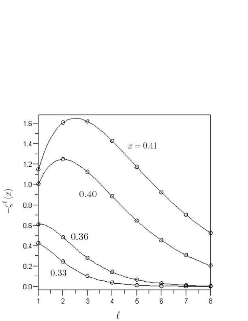
Figure 1: For various values of x, the convergence of $\eta^{\ell}{\rm(x)}$ and $\zeta^{\ell}{\rm(x)}$ in $\ell$ is shown. Note the difference in vertical scales.

IV.2 Conducting Star

So far, we have considered an insulating star which cannot be polarized. Now, we turn our attention to a conducting star which has free charges on it, but no net charge. Hence there could be non zero induced surface charge density. We call this surface charge density $\widetilde{\sigma}(\theta)$ (which can be decomposed as $\widetilde{\sigma}(\theta)=\Sigma_{\ell}\left[\widetilde{\sigma}^{\ell}P_{\ell}(\cos\theta)\right]$). This star would be polarized in such a way that the field inside it vanishes. The interior metric of the star plays no role in determining the field outside the star, only the size of the star $R_{s}$ matters. As before, $V=V^{\rm S}+\widetilde{V}$ is the total potential, $V^{\rm S}$ is the singular piece which exerts no self force and $\widetilde{V}$ (homogenous in the vicinity of the particle) is obtained by incorporating appropriate boundary conditions (namely zero field in the interior of the star, and zero net charge on its surface). Since the electric field is zero inside the star, the potential $V^{\rm S}+\widetilde{V}$ should be a constant on the surface of the star, hence $V_{\ell}^{\rm S}(R_{s})+\widetilde{V}_{\ell}(R_{s})=0$ for $\ell\neq 0$. For reasons already stated in section IV.1, $\widetilde{V}_{\ell}(R)=C_{\ell}f_{\ell}(R)$ outside the surface of the star. Using (18) for $V^{S}_{\ell}$, we can write

$$e\,g_{\ell}(R_{s})f_{\ell}(b)+C_{\ell}f_{\ell}(R_{s})=0:\qquad\ell\neq 0.$$ (42)

This equation can be solved to obtain $C_{\ell}$ for all $\ell\neq 0$.

$C_{0}$ can be obtained by imposing the condition that the net charge on the star vanishes, that is $\widetilde{\sigma}^{0}=0$. To impose this condition, we should first apply Gauss’s law to obtain an expression for the induced surface charges $\widetilde{\sigma}(\theta)$. Since the electric field inside the star vanishes, applying Gauss’s Law simply gives (see appendix A):

$$4\pi\widetilde{\sigma}(\theta)=-\left.R^{2}\frac{\partial V^{\rm S}(R,\theta)}{\partial R}\right|_{R=R_{s}}-\left.R^{2}\frac{\partial\widetilde{V}(R,\theta)}{\partial R}\right|_{R=R_{s}}$$ (43)

$$\Rightarrow 4\pi\widetilde{\sigma}^{\ell}=\left\{\begin{array}[]{cc}-R_{s}^{2}\left[e\,f_{\ell}(b){g_{\ell}}^{\prime}(R_{s})+C_{\ell}{f_{\ell}}^{\prime}(R_{s})\right]\neq 0&\text{for }\ell\neq 0\\ \vbox{\vskip 14.45377pt}-R_{s}^{2}\left[eM/R_{s}^{2}b-C_{0}/R_{s}^{2}\right]&\text{ for }\ell=0.\\ \end{array}\right.$$ (44)

In particular, using the fact that $\widetilde{\sigma}^{0}=0$, we find that $C_{0}=eM/b$. Note that $V_{0}(r)=2e/b$ for $r<r_{s}$.

IV.2.1 Evaluating the self force

Now that we know all the coefficients $C_{\ell}$, we have completely determined the regular field that would produce the self force. As in the previous section (insulating star), (35) gives the self force on the charge, with the only change being that the $C_{\ell}$ are now given by (42) rather than (33). So, the self force is

$$F_{\mathrm{self}}=\sum_{\ell}F_{\mathrm{self}}^{\ell}=-\frac{e^{2}M}{b}\,{f_{0}}^{\prime}(b)+e^{2}\sum_{\ell=1}^{\infty}\left(\frac{f_{\ell}(b)g_{\ell}(R_{s})}{f_{\ell}(R_{s})}\right){f_{\ell}}^{\prime}(b).$$ (45)

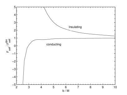
Figure 2: The self-force on the charge is plotted as a function of its position for the two cases considered in the text: when the star is an insulator (upper curve) and when it is a conductor (lower curve).

Observe that the result obtained for the self-force in (45) does not depend on the interior metric of the star.

To compare the results with that of the insulating star, we assume that the size of the star $R_{s}$ is the same as that of an extreme density star, $R_{s}={9M}/{4}$. Once again, it turns out that each $F_{\mathrm{self}}^{\ell}$ can be expressed as

$$F_{\mathrm{self}}^{\ell}=\frac{e^{2}}{b^{2}}\left[\frac{M}{b}\right]\zeta^{\ell}\left(\frac{M}{b}\right).$$ (46)

We again define $x={M}/{b}$ for convenience. The form of $\zeta^{\ell}(x)$ is given for $\ell=0,1,2$.

$$\zeta^{0}(x)=1,$$ (47)

$$\zeta^{1}(x) = -\frac{108}{x^{4}(72\ln 3-160)}\left(\frac{1}{2}\ln\left[1-2x\right]+x+x^{2}\right)$$ (48)

$$\times\left(-\left[\frac{1}{2}-x\right]\ln\left[1-2x\right]-x+x^{2}\right),$$

$$\zeta^{2}(x) = -\frac{900}{x^{6}(1080\ln 3-1376)}\left(\left[\frac{9}{2}x-3\right]\ln\left[1-2x\right]+x^{3}+3x^{2}-6x)\right)$$ (49)

$$\times\left(\left[\frac{3}{2}-\frac{9}{2}x+3x^{2}\right]\ln\left[1-2x\right]-6x^{2}+x^{3}+3x\right).$$

Whereas the $\eta^{\ell}(x)$ are positive for all values of $\ell$, the $\zeta^{\ell}(x)$ are negative for all $\ell$ except $\ell=0$. For large $\ell$, $\zeta^{\ell}(x)\rightarrow 0$, for all $x$. The convergence of $\zeta^{\ell}(x)$ is also plotted in Fig 1 for various values of $x$. We again note that as $x\rightarrow 0$ $(b\rightarrow\infty)$, we have $F_{\mathrm{self}}\rightarrow F_{\mathrm{self}}^{\mathrm{BH}}$; a charge placed far away from this star, would feel the same force as it would feel if the star were replaced by an equally massive black hole. However, something interesting happens nearby. There exists a point, $x_{0}$, where the charge feels zero self-force. This is an electrostatic equilibrium point. It happens when $\sum_{\ell=1}^{\infty}\zeta^{\ell}(x_{0})=-\zeta^{0}$. This condition can be numerically solved, giving $x_{0}=0.34$ $(b=2.95M)$. When $x<x_{0}$($b>2.95M$), the charge would experience a repulsive force and when $x>x_{0}$($b<2.95M$), the charge would experience an attractive force.

As an example, we shall numerically compute the force experienced by the charge placed at $x=0.42$.

$$F_{\mathrm{self}}=\frac{e^{2}}{b^{2}}\left[\frac{M}{b}\right]\Sigma_{\ell}\zeta^{\ell}(0.42)=-19.96\frac{e^{2}}{b^{2}}\left[\frac{M}{b}\right].$$ (50)

The closer we take the charge to the surface of the star, the more the attractive force increases. In the limit $x\rightarrow 4/9$, $F_{\mathrm{self}}\rightarrow-\infty$. This is expected because even in flat space, when a charge is placed close to a conductor, it experiences a huge attractive force. We should interpret the attractive force which dominates when the charge is close to the conducting star as a consequence of electrical polarization of the star and the repulsive force which dominates when the charge is far away from the star as due to interaction of the fields with space-time curvature. Fig 2 presents the self force experienced by the charge $F_{\mathrm{self}}$ (normalized with respect to $F_{\mathrm{self}}^{\mathrm{BH}}$) as a function of the position of the charge placed near a conducting and an insulating star.

A simple consistency check can be performed in the limiting case when $M\rightarrow 0$, by comparing it to the well known flat space limit. In flat space, the self force on the charge $e$ at a distance $b$ from the center of a conducting sphere of radius $R_{s}$ and zero net charge can be calculated to be

$$F_{\mathrm{self}}^{\mathrm{flat}}=\frac{e^{2}}{b^{2}}\left[\frac{1}{\left(1-\frac{R_{s}^{2}}{b^{2}}\right)^{2}}-1\right]\left(\frac{R_{s}}{b}\right).$$ (51)

In the limit $M\rightarrow 0$, (19,20) reduce to $f_{\ell}(R)\rightarrow 1/R^{\ell+1}$ and $g_{\ell}(R)\rightarrow R^{l}$. As a result (45) reduces to

$$F_{\mathrm{self}}=\frac{e^{2}}{b^{2}}\sum_{\ell=1}^{\infty}(\ell+1)\left(\frac{R_{s}}{b}\right)^{2\ell+1},$$

which exactly matches the flat space result (51).

Appendix A Gauss’s Law

In this appendix, we apply Gauss’s law to evaluate the charge density on the star’s surface. We start by reviewing Gauss’s law. Consider a spacelike 3-hypersurface $\Sigma$, bounded by a 2-surface $\partial\Sigma$. Then Gauss (Strokes) theorem can be written as poisson

$$\int_{\Sigma}\nabla_{\nu}F^{\mu\nu}\,d\Sigma_{\mu}=\frac{1}{2}\oint_{\partial\Sigma}F^{\mu\nu}dS_{\mu\nu}.$$ (52)

From Maxwell’s equations, the LHS corresponds to $-4\pi$ times $Q$, the total charge enclosed within the bounded region $\Sigma$. The surface element $dS_{\mu\nu}=-2n_{[\mu}\gamma_{\nu]}\sqrt{\sigma}d\theta d\phi$, where $n_{\mu}$ is the future directed unit normal to the space like hypersurface $\Sigma$ and $\gamma_{\nu}$ is the unit normal to the boundary $\partial\Sigma$. The vector $\gamma_{\nu}$ should always be directed away from the surface $\partial\Sigma$. The term $\sqrt{\sigma}d\theta d\phi$, represents the 2 dimensional surface area element.

In this paper, since we are interested in the surface charge density of the star, we apply Gauss’s law in a region very close the surface of the star. We choose the hypersurface $\Sigma$ to be a constant time $T$ (or $t$) hypersurface spatially bounded by the Gaussian surface $\partial\Sigma$, which is made up of two small pieces of constant-$R$ surfaces of coordinate area $d\theta d\phi$, one just outside the star surface $R=R_{s}$ (1) and the other just inside the star surface $r=r_{s}$ (8).

For the piece of $\partial\Sigma$ outside the star’s surface, in the Schwarzschild coordinate system $(T,R,\theta,\phi)$ as in metric (2), $n_{\mu}=(-\sqrt{1-2M/R},0,0,0)$ and $\gamma_{\mu}=(0,{1}/{\sqrt{1-2M/R}},0,0)$. The only nonvanishing component of $dS_{\mu\nu}$ is $dS_{TR}=R^{2}\sin\theta d\theta d\phi$. For the piece of $\partial\Sigma$ inside the surface of the star, $dS_{\mu\nu}$ is obtained from the unit normals to constant-$t$ and constant-$r$ surfaces with respect to the star’s interior metric. With respect to the star’s coordinate system $(t,r,\theta,\phi)$ as in metric (8), $n_{\mu}=(-(\beta^{2}+\alpha r^{2}),0,0,0)$ and $\gamma_{\mu}=(0,-1,0,0)$. Here, the only nonvanishing component of $dS_{\mu\nu}$ is $dS_{tr}=-(\beta^{2}+\alpha r^{2})r^{2}\sin\theta d\theta d\phi$.

By applying Gauss’s Law, (52), on $\Sigma$, we obtain,

$$-4\pi\sigma(\theta,\phi)\sin\theta d\theta d\phi=\left.g^{TT}g^{RR}F_{TR}dS_{TR}\right|_{\mathrm{R=R_{s}}}^{\mathrm{outside}}+\left.g^{tt}g^{rr}F_{tr}dS_{tr}\right|_{\mathrm{r=r_{s}}}^{\mathrm{inside}}.$$ (53)

Here, $\sigma(\theta,\phi)$ is the surface charge density and $\sigma(\theta,\phi)\sin\theta d\theta d\phi$ is the total charge contained within that small Gaussian surface. The axial symmetry of the problem considered in this paper ensures that $\sigma(\theta,\phi)$ is actually just $\sigma(\theta)$. We have adopted (53) in section IV of this paper. For the case of conducting star (section IV.2), we note that the field inside the star vanishes and hence the second term in the RHS of (53) vanishes.

A.1 Conformal invariance of Maxwell’s equations

As already indicated, we can ignore the conformal factor in (4) and use the metric (8) when evaluating the integral $\frac{1}{2}\int F^{\mu\nu}dS_{\mu\nu}$ on the surface just inside the star. This is justified as long as the source ($J^{\mu}\sqrt{-g}$) is conformally invariant, in which case:

• the LHS of (52) (that is, the total charge contained within a coordinate volume) is invariant under a conformal transformation,

• Maxwell’s equations have the same solution for the vector potential $A_{\mu}$, and hence the same solution for $F_{\mu\nu}$, in any conformally related metric.

Note that, under a conformal transformation $g_{\mu\nu}\!\rightarrow\!\Omega^{2}g_{\mu\nu}$ ($g^{\mu\nu}\!\rightarrow\!\Omega^{-2}g^{\mu\nu}$), so we also have $n_{\mu}\!\rightarrow\!\Omega n_{\mu}$, $\gamma_{\mu}\!\rightarrow\!\Omega\gamma_{\mu}$, $\sqrt{-g}\!\rightarrow\!\Omega^{4}\sqrt{-g}$ and $\sqrt{\sigma}\!\rightarrow\!\Omega^{2}\sqrt{\sigma}$. Hence,

$$dS_{\mu\nu}\rightarrow\Omega^{4}dS_{\mu\nu}.$$ (54)

Also note that, if the source ($J^{\mu}\sqrt{-g}$) is conformally invariant, Maxwell’s equations (10) require $F_{\mu\nu}$ to be conformally invariant. With contravariant indices $F^{\mu\nu}$ transforms under a conformal transformation as

$$F^{\mu\nu}=g^{\alpha\mu}g^{\beta\nu}F_{\alpha\beta}\rightarrow\frac{g^{\alpha\mu}}{\Omega^{2}}\frac{g^{\beta\nu}}{\Omega^{2}}F_{\alpha\beta}=\frac{1}{\Omega^{4}}F^{\mu\nu}.$$ (55)

Cleary, (54) and (55) imply that (52) is invariant under a conformal transformation.

References

References

- (1) J.M. Cohen and R.M. Wald, J. Math. Phys. 12, 1845 (1971).
- (2) R.S. Hanni and R.M. Ruffini, Phys. Rev. D8, 3259 (1973).
- (3) E.T. Copson, Proc. Roy. Soc. London A118, 184 (1928).
- (4) B. Linet, J. Phys. A9, 1081 (1976).
- (5) J. Hadamard, Lectures on Cauchy’s Problem (Yale University Press, New Haven, CT 1923).
- (6) P.A.M. Dirac, Proc. Roy. Soc. London A167, 148 (1938).
- (7) A.G. Smith and C.M. Will, Phys. Rev. D22, 1276 (1980).
- (8) B.S. DeWitt and R.W. Brehme, Ann. Phys. (N.Y.), 9, 220-259 (1960).
- (9) S. Detweiler and B.F. Whiting, Phys. Rev. D67, 024025 (2003).
- (10) L. Barack and A Ori, Phys. Rev. D61, 061502 (2000).
- (11) T.C. Quinn and R.M. Wald, Phys. Rev. D56, 3381 (1997).
- (12) L.M. Burko, Y.T. Liu and Y. Soen, Phys. Rev. D63, 024015 (2000).
- (13) C.M. DeWitt and B.S. DeWitt, Physics (Long Island City, N.Y.) 1, 3 (1964).
- (14) A.G. Wiseman, Phys. Rev. D61, 084014 (2000).
- (15) C.W. Misner, K.S. Thorne and J.A. Wheeler, Gravitation (Freeman, San Francisco 1973).
- (16) K. Shankar and B.F. Whiting, gr-qc/0706.4324.
- (17) G. Arfken, Mathematical methods for physicists 3rd ed (Academic Press, San Diego 1985).
- (18) E. Poisson, A relativists toolkit: The mathematics of black-hole mechanics (Cambridge University Press, Cambridge 2004).