Spectroscopic Analysis of H I Absorption Line Systems in 40 HIRES quasars

Abstract

We list and analyze H i absorption lines at redshifts 2 $<$ $z$ $<$ 4 with column density (12 $<$ $\log$($N_{\rm H\;I}$/[cm^-2]) $<$ 19) in 40 high-resolutional (FWHM = 8.0 km s^-1) quasar spectra obtained with the Keck$+$HIRES. We de-blend and fit all H i lines within 1,000 km s^-1 of 86 strong H i lines whose column densities are $\log N_{HI}$ $\geq$ 15 cm^-2. Unlike most prior studies, we use not only Ly$\alpha$ but also all visible higher Lyman series lines to improve the fitting accuracy. This reveals components near to higher column density systems that can not be seen in Ly$\alpha$. We list the Voigt profile fits to the 1339 H i components that we found. We examined physical properties of H i lines after separating them into several sub-samples according to their velocity separation from the quasars, their redshift, column density and the S/N ratio of the spectrum. We found two interesting trends for lines with 12 $<$ $\log$($N_{\rm H\;I}$/[cm^-2]) $<$ 15 which are within 200 – 1000 km s^-1 of systems with $\log$($N_{\rm H\;I}$/[cm^-2]) $>$ 15. First, their column density distribution becomes steeper, meaning relatively fewer high column density lines, at $z<2.9$. Second, their column density distribution also becomes steeper and their line width becomes broader by about 2–3 km s^-1 when they are within 5,000 km s^-1 of their quasar.

1 Introduction

Quasar absorption systems have historically been divided largely into three physically distinct categories: (i) absorption systems with strong metal lines arising in or near intervening galaxies, (ii) weak H i systems in the Ly$\alpha$ forest that come from the intergalactic medium, and (iii) intrinsic systems that are physically related to the quasars, including associated and broad absorption line systems.

Metal absorption systems usually contain H i lines with relatively large column densities, including two sub-categories: damped Lyman alpha (DLA) system and Lyman limit system (LLS) with H i column densities of $\log$($N_{\rm H\;I}$/[cm^-2]) $>$ 20.2 and 17.16, respectively. Deep imaging observations around quasars have provided evidences that the metal absorption systems are often produced in intervening galaxies. Galaxies have been detected that can explain Mg II absorption lines (e.g., Bergeron & Boissé 1991), and C IV absorption lines (e.g., Chen, Lanzetta, & Webb 2001).

On the other hand, nearly all H i lines have smaller column densities ($\log N_{HI}$ $\leq$ 15) than those associated found in gas that shows strong metal lines. The number of H i lines per unit $z$ increases with redshift (Peterson 1978; Weymann et al. 1998a; Bechtold 1994), because the intergalactic medium is denser and less ionized at higher $z$. The Ly$\alpha$ absorption lines are produced in intergalactic clouds (e.g., Sargent et al. 1980; Melott 1980), which are the higher density regions in the inter-galactic medium (IGM). The Ly$\alpha$ lines are broadened by Hubble flow (e.g., Rauch 1998; Kim et al. 2002a) as well as the Doppler broadening from the gas temperature.

Misawa et al. (2004) presented a study of H i absorption lines seen towards 40 quasars in spectra from the Keck HIRES spectrograph. In a departure from prior work, they considered the H i lines without considering the metal lines. They classified the H i lines as either high density lines [HDLs] which have or are near to strong H i lines that are probably related to galaxies, and low density lines [LDLs] that are far from any strong H i lines and are more likely to be far from galaxies and hence in the IGM.

Following Misawa et al. (2004), we define HDLs as all H i lines within $\pm$ 200 km s^-1 of a lines with $15$ $<$ $\log N_{HI}$ $<$ 19 cm^-2. We define LDLs as lines with 12 $<$ $\log N_{HI}$ $<$ 15 which are within 200 – 1000 km s^-1 of a line with $15<$ $\log N_{HI}$ $<$ 19  cm^-2. This last velocity constraint is intended to make the LDL a “control” sample for the HDLs, where the two samples come from similar redshifts and regions of the spectra with similar signal to noise.

Misawa et al. (2004) discovered that the HDLs have smaller Doppler parameters ($b$-values), for a given column density than the LDLs, and they also found the same effect in a hydrodynamic simulation with 2.7 kpc cells. Misawa et al. (2004) suggested that the LDLs are cool or shock-heated diffuse intergalactic gas, and that the HDLs are cooler dense gas near to galaxies.

Misawa et al. (2004) fit all the accessible transitions in the H i Lyman series to help de-blend H i lines. Their main sample comprised 86 H i absorption systems each with $\log N_{HI}$ $>$ 15 cm^-2. They also fit all H i lines within $\pm$1,000 km s^-1 of these H i lines, to give a total sample of 1339 H i lines, including the 86 lines. This is the only large sample in which multiple Lyman series lines are fit together, although this method has been used on individual systems and small samples (Songaila et al. 1994; Tytler, Fan, & Burles 1996; Wampler et al. 1996; Carswell et al. 1996; Songaila et al. 1997; Burles & Tytler 1998a,1998b, Burles, Kirkman, & Tytler 1999; Kirkman et al. 2000; O’Meara et al. 2001; Kirkman et al. 2003; Kim et al. 2002b; Janknecht et al. 2006).

In this paper, we present measurements of the absorption lines that Misawa et al. (2004) have analyzed. We give a detailed description of each absorption system and we summarize new results. The paper is organized as follows: In §2, we give descriptions of the data and the line fitting. The results of our statistical analyses are presented in §3. We discuss our results in §4, and summarize them in §5. In the Appendix, we describe the properties and we give velocity plots for each H i system. We use a cosmology in which $H_{0}=72$ km s^-1Mpc^-1, $\Omega_{m}$ = 0.3, and $\Omega_{\Lambda}$ = 0.7.

2 Spectra and Line Fitting

The 40 quasars in our sample have either DLA systems or LLSs, and they were observed as a part of a survey for measurements of the deuterium to hydrogen (D/H) abundance ratio. The detailed description of the absorption and data reduction are presented in Misawa et al. (2004). We caution that our sample was biased in subtle ways by the selection of LLS and DLAs that seemed more likely to show D, i.e. those with simpler velocity structure.

We list the 40 quasars in Table 1. Column (1) is the quasar name, (2) the emission redshift. Columns (3) and (4) are the optical magnitude in the $V$ and $R$ bands. The lower and upper wavelength limits of the spectra are presented in columns (5) and (6). Column (7) gives the S/N ratio at the center of the spectrum. Same data set was also used in Misawa et al. (2007) in a study of the quasar intrinsic absorption lines.

We will discuss only H i lines with $\log N_{HI}$ $>$ 15 cm^-2 and other H i weaker lines within $\pm$1,000 km s^-1 of these strong H i lines. We selected this velocity range since it is enough to include the conspicuous clustering of strong metal lines. Indeed such strong metal lines are normally confined to an interval of $<400$ km s^-1 even for DLA systems (Lu et al. 1996b).

Here we briefly review the line detection and fitting procedures that we discussed in more detail in Misawa et al. (2004). We began searching the literature for H i lines with $\log N_{HI}$ $>$ 15, including the DLA and LLS catalogues (Sargent, Steidel, & Boksenberg 1989, hereafter SSB; Lanzetta 1991; Tytler 1982), and metal absorption systems (Péroux et al. 2001; Storrie-Lombardi et al. 1996; Petitjean, Rauch, & Carswell 1994; Lu et al. 1993; Steidel & Sargent 1992; Lanzetta et al. 1991; Barthel, Tytler, & Thomson 1990; Steidel 1990a,b; Sargent, Boksenberg, & Steidel 1988, hereafter SBS; SSB). We also search for them ourselves. If more than one strong H i line was detected in a single 2000 km s^-1 velocity window, we take the position of the H i line with the largest column density (hereafter the “main component”) as system center. We found 86 H i systems with $\log N_{HI}$ $>$ 15, at 2.1 $<$ $z_{abs}$ $<$ 4.0, in 31 of the 40 quasars. Figure 1 of Misawa et al. (2004) gives the velocity plot of one of these systems, and below we give the rest.

We give parameters describing these 86 systems in Table 2. In successive columns list (1) the name of the quasar; (2) the redshift of the main component, that with the largest column density ; (3) the H i column density of the main component $N_{1}$; (4) $N_{2}$, the second largest H i column density within $\pm 1000$ km s^-1 of the main component; (5) the ratio of $N_{2}$ to $N_{1}$; (6) – (9) the S/N ratios at Ly$\alpha$, Ly$\beta$, Ly$\epsilon$, and Ly10; (10) the number of lines in the $\pm$ 1,000 km s^-1 window; (11) the number of H i lines classified as HDLs (described later); (12) comments on the H i system; (13) references. We will call this list sample S0 (Table 3).

When we were fitting the lines, we rejected narrow lines with Doppler parameter of $b$ $<$ 4.8 km s^-1, which corresponds to the resolution of our spectra. We also identify all lines with $b$ $<$ 15 km s^-1 as possible metal lines (called M I in Tables) because H i lines with this narrow width are rare (e.g., Hu et al. 1995, hereafter H95; Lu et al. 1996a, hereafter L96; Kirkman & Tytler 1997a, hereafter KT97). If there was more than one way to fit the lines, we chose the fit with the fewest lines. If the model did not give good fits to all the Lyman series lines, we adopted the model that best fit the lower order lines where the SNR is best. For H i lines with column densities of $\log N_{HI}$ $\geq$ 16.6 the Lyman continuum optical depth is $\tau$ $\geq$ 0.25. For these systems we checked if the residual flux at the Lyman limit was consistent. Our fitting method could readily overestimate the Doppler parameter but not the column density. Once the fitting model is chosen, we used $\chi^{2}$ minimization in a code written by David Kirkman, to get the best fit parameters of H i column density ($\log N_{HI}$), Doppler parameter ($b$), and absorption redshift ($z$). The internal errors are typically $\sigma$($\log N_{HI}$)=0.09 cm^-2, $\sigma$($b$)=2.1 km s^-1, and $\sigma$($z$)=2.5$\times$$10^{-5}$.

We prepared a sample S1 that is a sub-sample of S0 including only 973 H i lines and 61 H i systems with $\log N_{HI}$ $>$ 15. S1 excludes 25 systems with difficulties such as (i) poor fitting due to gaps in the echelle formatted spectra, (ii) poor fitting due to strong DLA wings (i.e., $\log N_{HI}$ $>$ 19), (iii) close proximity in redshift to the background quasars (i.e., within 1,000 km s^-1 of the emission redshift), and (iv) overlapping with other H i systems. The S/N ratios of the spectra are at least S/N $\simeq$ 11 per 2.1 km s^-1 pixel and the mean value is S/N $\simeq$ 47 for Ly$\alpha$ lines. Among these 61 H i systems, three systems may be physically associated with the quasars based on the partial coverage analysis for the corresponding metal absorption lines (Misawa et al. 2007). However, we keep these systems in S1 sample, because we still cannot reject the idea that they are intervening systems.

We give detailed descriptions of all the lines that we fit in the Appendix. We also give velocity plots of the first five Lyman transitions, Ly$\alpha$, Ly$\beta$, Ly$\gamma$, Ly$\delta$, and Ly$\epsilon$.

3 RESULTS

We investigate the properties of line parameters such as the column density, Doppler parameter, and the clustering properties of the H i lines. Since this sample contains not only H i lines originating in the intergalactic diffuse gas clouds (i.e., LDLs), but also H i lines produced by intervening galaxies (i.e., HDLs), we also attempted to separate H i lines into HDLs and LDLs based on the clustering trend (Misawa et a. 2004).

Our analysis is similar to that of previous studies (e.g., H95; L96; KT97), but with three key differences: (i) earlier studies used all H i lines detected in the quasar spectra, whereas we use only H i lines within $\pm$ 1,000 km s^-1 of the main components with $\log N_{HI}$ $\geq$ 15, (ii) our sample contains a number of strong lines ($\log N_{HI}$ $\geq$ 15) in addition to weak H i lines ($\log N_{HI}$ $<$ 15), and (iii) our sample covers a wide redshift range: 2.0 $\leq$ $z_{abs}$ $\leq$ 4.0. The redshift distributions of the 86 and 61 H i systems in samples S0 and S1 are shown in Figure 1.

3.1 Sub-Samples for the Statistical Analysis

For further investigation, we prepared several sub-samples as follow. It is known that the comoving number densities of low-ionization lines, such as H i lines, decreases in the vicinity of quasars (Carswell et al. 1982; Murdoch et al. 1986; Tytler 1987). This trend is known as the “proximity effect”, and is probably caused by the enhanced UV flux from the quasar towards which the absorption is seen. We separate the 61 H i systems (sample S1) into sub-samples S2a (the velocity difference from the quasar, $\Delta v$ $>$ 5,000 km s^-1) and S2b ($\Delta v$ $<$ 5,000 km s^-1). We have already removed from S1 all H i systems within 1,000 km s^-1 of the quasars to avoid H i systems from the quasar host galaxies.

H95 emphasized that the line detection limit is almost wholly determined by the line blending (or blanketing), and not by the S/N ratio of the spectrum. In order to confirm whether the distribution of line parameters is affected by the quality of the spectrum, we made two overlapping samples from S1 using the S/N ratio of each spectrum in the Ly$\alpha$ region: S3a (S/N $\geq$ 40), and S3b (S/N $\geq$ 70). These sub-samples include 34 ($\sim$ 60%) and 17 ($\sim$ 30%) of the 61 H i systems of the sample S1.

Sample S1 covers a broader range of redshifts, $2.0<z<4.0$, when compared with previous studies: $2.55<z<3.19$ for H95, $3.43<z<4.13$ for L96, and $2.43<z<3.05$ for KT97. When we investigate the redshift evolution of H i absorbers, we also divided S1 into two sub-samples; S4a ($z<2.9$) and S4b ($z\geq 2.9$). Here the two sub-samples have nearly the same number of H i systems.

Finally, we made sub-samples according to the column densities of H i lines, as the distributional trends of strong and weak H i lines are very different (see Figure 2 in Misawa et al. 2004); the H i lines with relatively large column densities tend to cluster around the main components, while the number of weak H i lines decreases near the center of H i systems because of line blanketing. Since one of our interests is to determine the boundary value of column density between HDLs and LDLs (although other parameters may be necessary to separate them), we separate the 973 H i lines into eight sub-samples according to their column densities. We use boundary values of $\log N$ = 13, 14, 15, and 16, where sub-sample S5_ab contains H i lines whose column densities are $\log$($N_{\rm H\;I}$/[cm^-2]) values of a to b.

In Table 3 we summarize these 16 sub-samples. Here we should emphasize that S5₁₂₁₃, S5₁₂₁₄, S5₁₂₁₅, S5₁₂₁₆, S5₁₃₁₉, S5₁₄₁₉, S5₁₅₁₉, and S5₁₆₁₉, are separated by the properties of lines, while S2a, S2b, S3a, S3b, S4a, and S4b are separated by the unit of system.

3.2 Physical Properties of H i Absorbers

For each sub-sample prepared in the last section, we perform statistical analysis, including analysis of the column density distribution, Doppler parameter distribution, and line clustering properties. The samples used here contain both HDLs and LDLs.

3.2.1 Column Density Distribution

The column density distribution of H i lines, $dn(N)/dN$, are usually fit with a power law (Carswell et al. 1984, Tytler 1987, Petitjean et al. 1993; H95),

$$\log\left(\frac{{\rm d}n(N)}{{\rm d}N}\right)=-\beta\hskip 2.84526pt\log N+A,$$ (1)

where the index $\beta$ was estimated to be 1.46 (H95), 1.55 (L96), and 1.5 (KT97) with only weaker H i lines with $\log N_{HI}$ = 12 – 14.5. Janknecht et al. (2006) found $\beta$ = 1.60$\pm$0.03 at lower redshift $z$ $<$ 1.9. The column density distributions of our seven sub-samples (S1, S2a, S2b, S3a, S3b, S4a and S4b) per unit redshift and unit column density are analyzed. The plot in Figure 2 is the result for sub-sample S1. Since the turn-over of the distribution around $\log N_{HI}$ = 12.5 is probably due to line blending and/or blanketing as described later in § 4, we fit the column density distributions only for $\log N_{HI}$ $>$ 13. The best-fitting parameters, $\beta$ and $A$, as well as the redshift bandpass, $\Delta z$, of each sub-sample are summarized in Table 4, along with the past results from KT97 and Petitjean et al. (1993).

The indices that we find, $\beta$ = 1.40$\pm$0.03, are slightly smaller than the value in the past results, $\beta$ = 1.46 –1.55, which means that our sample favors strong H i lines. But we expect this type of trend. Our samples contain not only LDLs but also HDLs, and since we cover only the velocity regions within $\pm$ 1,000 km s^-1 of the main components, we have a strong excess of strong H i lines. We see the column density distribution does not change with the velocity distance from the quasars (S2a and S2b) or with the S/N ratio (S3a and S3b), but it is weakly affected by redshift (S4a and S4b). We also applied the Kolmogorov-Smirnov (K-S) test to the sub-samples. The results in Table 5 show that we can not rule out the hypothesis that they are random samplings from the same population.

3.2.2 Doppler Parameter Distribution

The distribution of the Doppler parameter of H i lines have been approximately given by the truncated Gaussian distribution (H95; L96),

$$\frac{{\rm d}n(b)}{{\rm d}b}=\left\{\begin{array}[]{ll}A\;\exp\left[\frac{-(b-b_{0})^{2}}{2\sigma_{b}^{2}}\right]&b\geq b_{min}\\ 0&b<b_{min}\end{array}\right.$$ (2)

where $b_{0}$ and $\sigma_{b}$ are the mean and the dispersion of $b$ distribution and $b_{min}$ is the minimum $b$ value for an H i line. There are two origins of line broadening: thermal broadening ($b_{T}$), and micro-turbulence ($b_{tur}$). The total amount of broadening is given by $b=\sqrt{b_{T}^{2}+b_{tur}^{2}}$.

In order to determine the correct Doppler parameter, we have to individually resolve and fit H i lines using Voigt profiles. However, most of weak H i lines disappear in the observed spectrum due to line blending and blanketing, especially near strong lines. To derive the intrinsic (as opposed to observed) distribution of the Doppler parameter, previous authors (i.e., H95; L96; KT97) have chosen artificial H i lines (as input data) with distributions characterized by a Gaussian, and used them for comparison with the observed distributions. KT97 noted that the $b$-value distribution of lines seen in simulated spectra resembles the distribution of the input data, except for two differences: (i) an excess of lines with large $b$-values is seen in the recovered data, compared to the input data, which is probably produced by line blending, and (ii) lines with very small $b$-values ($b$ $<$ 15 km s^-1) are found, which are probably data defects or noise, as they are not present in the input data. Nonetheless, the $b$-value distribution of the input and recovered data resemble each other between $b$ = 20 km s^-1 and $b$ = 60 km s^-1.

We would ideally like to determine the real distribution of Doppler parameters; however, the only way to do this is to perform simulations, and compare the recovered Doppler parameter distribution with the observed distribution. Such simulations are expensive to perform, so in this work we simply compared the distribution in our sample with the past results of H95 and L96 at $b$ = 20 – 60 km s^-1. We analyzed the observed distributions of Doppler parameters for 15 sub-samples, and compare them with the results in H95 ($b_{0}$ = 28 km s^-1, $\sigma_{b}$ = 10 km s^-1, and $b_{min}$ = 20 km s^-1) and L96 ($b_{0}$ = 23 km s^-1, $\sigma_{b}$ = 8 km s^-1, and $b_{min}$ = 15 km s^-1), where the parameters are the inputs used for artificial spectra that reproduce the observed distribution.

We see an excess of H i lines with large $b$-values of $b$ $>$ 50 km s^-1 in all of the sub-samples, while we have no lines with $b$ $\leq$ 15 km s^-1 because we decided to classify them into metal lines. All sub-samples except for $S_{1213}$ have relatively large $b$-values, and their distributions are closer to H95’s distribution than L96’s. In contrast, the distribution of $S_{1213}$, containing only H i lines with small column densities, $\log N_{HI}$ $<$ 13, resembles L96’s distribution. We plot in Figure 3 the Doppler parameter distributions of sub-samples S1 and S₁₂₁₃. We also applied a K-S test to the sub-samples (S2a, S2b, S3a, S3b, S4a, and S4b). The results are listed in Table 6. The probability, that the distributions of sub-samples S2a ($\Delta v$($z_{em}$$-$ $z_{abs}$) $>$ 5000 km s^-1) and S2b ($\Delta v$($z_{em}$$-$ $z_{abs}$) $\leq$ 5000 km s^-1) were drawn from the same parent population, is very small, $\sim$2.4 %. This result could suggest that the Doppler parameters of H i lines within 5000 km s^-1 of quasars are affected by UV flux from the quasars.

3.3 HDLs and LDLs

In the previous section, we carried out statistical analysis using sub-samples containing both HDLs and LDLs together. Here, we repeat these tests on the two samples separately.

Metal absorption lines seen in DLA systems or LLSs are strongly clustered within several hundred km s^-1, which implies their relationship to galaxies. In simulations Davé et al. (1999) also noted that galaxies tend to lie near the dense regions that are responsible for strong H i lines. On the other hand, for weak H i lines, no strong clustering is seen (e.g., Rauch et al. 1992; L96; KT97), although some studies found only weak clustering trends (e.g., Webb 1987; H95; Cristiani et al. 1997).

As Misawa et al. (2004) found, lines with $\log N_{HI}$ $\geq$ 15 show strong clustering trends at $\Delta v$ $<$ 200 km s^-1, while lines with lower column densities cluster weakly at $\Delta v$ $<$ 100 km s^-1 (Figure 4).

Misawa et al. (2004) defined HDLs as H i lines with $15$ $<$ $\log N_{HI}$ $<$ 19 and other weaker H i lines within $\pm$ 200 km s^-1 of those stronger H i lines. They then defined the LDLs as all other lines with 12 $<$ $\log N_{HI}$ $<$ 15. They chose $\log N_{HI}$ = 15  cm^-2 in the definition because the two point correlation was largest for a sub-sample of H i lines with 15 $<$ $\log N_{HI}$ $<$ 19. We list the number of HDLs and LDLs in the sub-samples in Table 7.

3.3.1 Column Density Distribution

In Table 8 we give the parameters that describe the column density distributions of HDLs and LDLs for five sub-samples (S1, S2a, S2b, S4a, and S4b). The most obvious result is that the HDLs have a smaller index than the LDLs. We see the same result in Figure 3 of Petitjean et al. (1993), and hence we now confirm this with the first large sample to consider the sub-components of the HDLs.

The distributions of LDLs in sample S1, S2a, and S4b are almost consistent with the previous result in KT97. On the other hand, the power law indices for the LDLs of S2b ($\Delta v$ $\leq$ 5000 km s^-1) and S4a ($z$ $<$ 2.9), $\beta$ = 1.90$\pm$0.16 and 1.71$\pm$0.06, are larger than the values for the other sub-samples, $\beta\sim$ 1.52, which means that LDLs at lower redshift or near the quasars tend to have lower column densities compared with those at higher redshift or far from the quasars. The change in the column density distribution near to the quasars may be just a consequence of the enhanced UV radiation.

3.3.2 Doppler Parameter Distribution

The Doppler parameter distributions of HDLs and LDLs for sub-samples (S1, S2a, S2b, S4a, and S4b) are also investigated, and the results of K-S tests applied to them are summarized in Table 9. The only remarkable result is that the probability, that the Doppler parameter distributions of LDLs at $\Delta v$ $>$ 5,000 km s^-1 (S2a) and $\Delta v$ $\leq$ 5,000 km s^-1 (S2b) from the quasars were drawn from the same parent population, is very small, $\sim$2.0%. We shows these two distributions in Figure 5. In Figure 6 we see that the cumulative distribution for the line $b$-values rises more slowly for the LDLs near to the quasars (at $\Delta v$ $\leq$ 5000 km s^-1), which means that these lines near to the quasars are broader by about 2–3 km s^-1. For other pairs of the sub-samples, we could not rule out the hypothesis that their parent populations are same.

4 Discussion

In this section, we discuss our results, especially the fact that the column density distribution is changing with the redshift and the velocity distance from the quasars. We also compare our results to those at lower redshift ($z$ $<$ 0.4) from the literature. After that, we also briefly discuss the completeness of H i lines in our 40 spectra.

4.1 Redshift Evolution of H i Absorbers

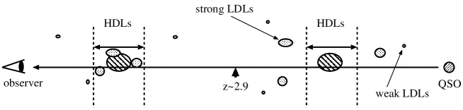
Figure 8: Cartoon of the distribution of absorbers at $z$ $\geq$ 2.9 and $z$ $<$ 2.9. Shaded circles are HDL absorbers. Dotted and small circles are strong (e.g., $\log N_{HI}$ $>$ 14.5) and weak (e.g., $\log N_{HI}$ $<$ 14.5) LDL absorbers, respectively. If strong LDL absorbers would gather around HDL absorbers within relative velocity of $\Delta v$ $<$ 200 km s^-1, the number of strong LDLs decrease as redshift decreases. Such trend is consistent with the concept of the hierarchical clustering model.

In § 3, we prepared two sub-samples, S4a and S4b, to compare the physical properties of H i lines at lower redshift ($z_{abs}$ $<$ 2.9) and at higher redshift ($z_{abs}$ $\geq$ 2.9). We do not see a change in the column density distribution in the sample as a whole, but once they are separated into HDLs and LDLs, we notice that the index of the column density distribution of LDLs at $z_{abs}$ $<$ 2.9 ($\beta$ = 1.71$\pm$0.06) is clearly different from that of LDLs at $z_{abs}$ $\geq$ 2.9 ($\beta$ = 1.52$\pm$0.09). On the other hand, there was no redshift evolution for HDLs. This trend, shown in Figure 7, means that there is a deficit of relatively stronger LDLs (i.e., $\log N_{HI}$ $\geq$ 14.5) at lower redshift. One of the possible explanations is that at lower redshift, more H i lines with the column densities just below $\log N_{HI}$ = 15 (i.e., relatively strong LDLs) might be associated with HDLs. In other words, stronger (i.e., $\log N_{HI}$ = 14.5 – 15) LDLs get into within 200 km s^-1 of the nearest HDLs, and would be classified into HDLs, which is consistent with the trend expected in the hierarchical clustering model (Figure 8).

As for the Doppler parameter distribution, we did not find any remarkable redshift evolutions in neither HDLs nor LDLs. L96 claimed that there is a redshift evolution of the Doppler parameter between $z$ = 2.8 and 3.7; the mean value of Doppler parameter at $z_{abs}$ = 3.7 ($b_{0}$ = 23 km s^-1; L96) is smaller than the value at $z_{abs}$ = 2.8 ($b_{0}$ = 28 km s^-1; H95). The corresponding value in KT97 ($b_{0}=23$ km s^-1) is, however, different from the result in H95. The difference may be due to the different line fitting procedure used in these studies; L96 and KT97 used the VPFIT software, while H95 used different software. Especially important is how the authors chose to treat blended lines. The difference could be related to the difference of the spectrum resolutions; R=45000 (L96; KT97) and R=36000 (H95). Janknecht et al. (2006) did not detect any evolution on the Doppler parameter at $z$ = 0.5 – 1.9. Our results, which are based on the data set taken with one observational configuration and fit using the same procedure, suggests that the Doppler parameter distribution of H i clouds does not evolve with redshift at $z$ = 2 – 4.

4.2 Proximity Effect near Quasars

It has long been noted that the number of Ly$\alpha$ lines decreases near to the redshift of the quasars (Carswell et al. 1982; Murdoch et al. 1986; Tytler 1987). This phenomenon is related to the local excess of UV flux from the quasars. The proximity effect has been used to evaluate the intensity of the background UV flux. Bajtlik et al. (1988) first measured the mean intensity of the background UV intensity, $J_{\nu}$ = $10^{-21.0\pm 0.5}$ (erg s^-1 cm^-2 Hz^-1 str^-1) at the Lyman limit at 1.7 $<$ $z$ $<$ 3.8, by estimating the distance from the quasar at which the quasar flux is equal to the background UV flux. The typical radius is $\sim$ 5 Mpc in physical scale that corresponds to the velocity shift of $\Delta v$ $\sim$ 4,000 km s^-1 from the quasars. L96 also evaluated the background UV intensity to be $J_{\nu}$ = $2\times 10^{-22}$ (erg s^-1 cm^-2 Hz^-1 str^-1) at $z$ $\sim$ 4.1 in the spectrum of Q0000-26.

We see two differences in LDLs within 5,000 km s^-1 of the quasars, compared to those far from the quasars ($\Delta v$ $>$ 5,000 km s^-1). We see fewer strong LDLs leading to a large index for the column density power law, $\beta$ = 1.90$\pm$0.16 (Figure 9). We also see that the distribution of Doppler parameter is different from that of H i lines far from the quasars at 98.8 % confidence level. The lines near to the quasar apparently tend to have broader lines (Figures 5 and 6), although this is a tentative result because we consider few lines near to the quasars.

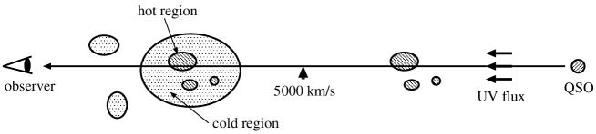
Figure 10: Cartoon of the distribution of absorbers far from the quasars ($\Delta v$ $>$ 5000 km s^-1) and near the quasars ($\Delta v$ $\leq$ 5000 km s^-1). Shaded regions are dense regions that are adiabatically compressed and heated, while dotted regions are diffuse cold regions. If LDL absorbers near the quasars are strongly affected by the UV flux from the quasars, H i gas at the diffuse cold regions would be preferentially ionized. As a result, stronger LDLs would become to be weaker LDLs and only central hot regions are observed, which makes the relative frequency of stronger LDLs smaller and the mean $b$ value of LDLs larger.

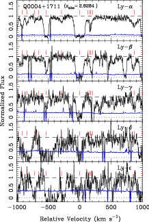
Figure 11: (Sample) Velocity maps of the lowest five orders of Lyman series (i.e., Ly$\alpha$, Ly$\beta$, Ly$\gamma$, Ly$\delta$, and Ly$\epsilon$) in a H i system at $z_{abs}$ = 2.8284 in the spectrum of Q0004+1711. A histogram just above the zero flux is 1$\sigma$ error spectrum. Tick marks above the flux spectrum denote the positions of H I and M I lines. Metal lines in the velocity window are not marked because they are not physically related to the H i system.

These results could be accounted for by assuming a two-phase structure: outer cold low-density regions and inner hot high-density regions in which temperature is determined by the competition between photoionization heating and adiabatic cooling. When gas is near to the quasars, the outer regions become too highly ionized to show much H I, and only the inner hot regions would be observed in H I, which would increase the mean value of the Doppler parameter. The increased ionization also decreases the total column densities of H I gas compared with gas far from the quasars (Figure 10). As reported in the past observations (e.g., Kim et al. 2001; Misawa et al. 2004), $\log N_{HI}$ and $b$(H i) have a positive correlation for $\log N_{HI}$ $<$ 15. This correlations was also reproduced by hydrodynamical simulations (e.g., Zhang et al. 1997; Misawa et al. 2004). These results suggest that high density regions tend to have larger Doppler parameters, if the absorbers are not optically thick. Davé et al. (1999) also presented an interesting plot in their Figure 11 that supported there existed three kinds of phases for H i absorbers (diffuse, shocked, and condensed phases). Among them, the diffuse phase whose volume densities are small (i.e., it corresponds to LDLs in our paper) has a positive correlation between $\log N_{HI}$ and $b$. On the other hand, an anti-correlation between $\log N_{HI}$ and $b$ is seen only for the condensed phase with high volume density that is probably associated with galaxies. The shocked phase, probably consisting of shock-heated gas in galaxies, does not show any remarkable correlations between them. Thus, if we assume all LDLs in our sample arise in the diffuse phase absorbers, our scenario above could reproduce the difference between sub-samples S2a and S2b.

4.3 Comparison to H i Absorbers at Lower Redshift

The number density evolution of H i absorbers (i.e., $dN/dz$ $\propto$ $(1+z)^{-\gamma}$) has been known to slow dramatically at $z$ $\sim$ 1.6, from a high-$z$ rapid evolution with $\gamma$ of 1.85$\pm$0.27 (Bechtold 1994) to a low-$z$ slow evolution with $\gamma$ of 0.16$\pm$0.16 (Weymann et al. 1998b). This trend is suggested to be due to the decline in the extragalactic background radiation using hydrodynamic cosmological simulations (e.g., Theuns, Leonard, & Efstathiou 1998). Thus, a comparison of H i absorbers at high-$z$ and local universe is another interesting topic.

In § 3, we found that the column density distribution of LDLs at $z$ $<$ 2.9 ($\beta$ = 1.71$\pm$0.06) is steeper than that at $z$ $>$ 2.9 ($\beta$ = 1.52$\pm$0.09). We proposed this trend could be due to the hierarchical clustering. If the assembly of structure in the IGM indeed dominates the column density distribution, we would expect to find a steeper column density distributions at lower redshift as proposed in § 4.1.

Using the Hubble Space Telescope (HST) and the Far Ultraviolet Spectroscopic Explorer (FUSE), Penton, Stocke, & Shull (2004) and Lehner et al. (2007) estimated power-law indices to be $\beta$ of 1.65$\pm$0.07 at 12.3 $\leq$ $\log N_{HI}$ $\leq$ 14.5 and 1.76$\pm$0.06 at 13.2 $\leq$ $\log N_{HI}$ $\leq$ 16.5 at $z$ $<$ 0.4, respectively. On the other hand, Davé & Tripp (2001) found a flatter distribution ($\beta$ = 2.04$\pm$0.23) at $z$ $<$ 0.3. The latter steeper distribution was also reproduced by hydrodynamical simulations (e.g., Theuns et al. 1998). If we accept the steeper result, the column density distribution would continue to be steeper as going to the lower redshift, which supports our idea that the hierarchical clustering could play a main role of the evolution seen in the column density distribution, although extragalactic radiation would contribute to play a role.

Absorption line width is another parameter that is still in argument whether it would evolve with redshift or not, as mentioned in § 4.1. While most of the space-based ultraviolet observations could not measure line widths by model fittings because of the lacks of spectral resolutions, Lehner et al. (2007) for the first time measured Doppler parameters of H i absorption lines accurately at lower redshift ($z$ $<$ 0.4), and investigate their distributional trend. By comparing to the results at higher redshift, Lehner et al. (2007) discovered that Doppler parameters are monotonously increasing from $z$ = 3.1 to $\sim$0. Such a trend was not confirmed in past papers (e.g., Janknecht et al. 2006). The fraction of the broad Ly$\alpha$ absorbers (BLA; $b$ $\geq$ 40 km s^-1) is also confirmed to increase by a factor of $\sim$3 from $z$ $\sim$ 3 to 0 (Lehner et al. 2007). Here, $b$ = 40 km s^-1 corresponds to gas temperature of $T_{gas}$ $\sim$ $10^{5}$ K, which is a border between the cool photoionized absorbers and the highly ionized warm-hot absorbers. These results suggests that a large fraction of H i absorbers at very low redshift (i.e., $z$ $<$ 0.4) are hotter and/or more kinematically disturbed than at higher redshift (i.e., $z$ $>$ 2.0).

In our sample,we do not see any clear difference of mean/median Doppler parameter at $z$ $\geq$ 2.9 ($b_{mean}$ = 31.0$\pm$10.0, $b_{med}$ = 28.1) and $z$ $<$ 2.9 ($b_{mean}$ = 32.0$\pm$10.9, $b_{med}$ = 29.6). Neither HDLs nor LDLs shows any evolutional trends. These negative results could be because with our optical data we covered only higher redshift regions than $z$ $\sim$ 1.6, at which $dN/dz$ evolution dramatically changed. Similarly, the fraction of the BLA ($f_{BLA}$ = 0.182 at $z$ $\geq$ 2.9 and 0.196 at $z$ $<$ 2.9) shows an only marginal hint to the evolution. However, these fractions are consistent to the result from KT97 ($f_{BLA}$ = 0.179; Lehner et al. 2007) at 2.43 $<$ $z$ $<$ 3.05 that is similar redshift coverage as our sample. Thus, Doppler parameter could increase as going to the lower redshift, but such a trend would be remarkable only if we trace its distribution at very low redshift (at $z$ $<$ 0.4) and compare it to that at much higher redshift (at $z$ $>$ 2).

As for the clustering trend of H i absorption lines, we see a very similar property at low and high redshift regions. As presented in Figure 4, we found a strong clustering trend within $\Delta v$ of 200 km s^-1 for H i lines with $\log N_{HI}$ between 15 and 19, while only a weak correlation is seen for weaker H i lines within $\Delta v$ of 100 km s^-1. Penton et al. (2004) presented very similar results: 5$\sigma$ (7.2$\sigma$) excess within $\Delta v$ of 190 km s^-1 (260 km s^-1) and only stronger H i lines contribute to this clustering. Penton, Stock, & Shull (2002) proposed such clustering trends within several hundreds of km s^-1 are due to clusters of galaxies. There could exist similar kinematical structures both at high-$z$ and in local universe.

4.4 Completeness of H i Line Sample

For a statistical analysis, especially the number density analysis, the completeness of the H i line detection is influenced by the detection limit of absorption lines (e.g., equivalent width or column density). In this study, we have used the H i lines detected in the 40 HIRES spectra that have various S/N ratios. The strong line sample will have subtle biases arising from the selection of the quasars because they were once thought to be good targets for the detection of deuterium. For example, we avoided quasars with no LLSs, and we avoided LLSs with previously known complex velocity structure. Nevertheless, we confirmed that our sample is almost complete for weak lines in the following way.

The minimum detectable equivalent width in the observed-frame, $W_{min}$, can be estimated using the following relation,

$$U=\frac{W_{min}N_{C}}{\sigma(W_{min}N_{C})}=\frac{W_{min}(S/N)}{(M_{L}^{2}M_{C}^{-1}+M_{L}-W_{min})^{1/2}},$$ (3)

where $M_{L}$ and $M_{C}$ are the numbers of pixels over which the equivalent width and the continuum level ($N_{C}$) are determined (Young et al. 1979; Tytler et al. 1987). The value of ($S/N$) is the S/N ratio per pixel. When we set $U\simeq W/\sigma(W)$ is 4 (i.e., 4$\sigma$ detection), the eqn.(3) can be solved to give,

$$W_{min} = (S/N)^{-2}\{[64+16(S/N)^{2}\times$$ (4)

$$(M_{L}+M_{L}^{2}/M_{C})]^{1/2}-8\}\times\Delta\lambda\hskip 5.69054pt(\rm{\AA}),$$

where $\Delta\lambda$ is the wavelength width per pixel in angstroms (Misawa et al. 2002). Here, we set $M_{L}$ for 2.5 times FWHM of each line, and $M_{C}$ for full width of each echelle order. Once the minimum rest-frame equivalent width, $W_{rest}[=W_{min}/(1+z)]$, has been evaluated, it can be converted to the minimum column density by choosing a specific Doppler parameter; the result is insensitive to the choice on the linear part of the curve of growth. Among the 86 H i systems in our data sample, the H i system at $z_{abs}$ = 2.940 in the spectrum of Q0249-2212 is located in the region with the lowest S/N ratio (i.e., $S/N$ $\sim$ 11). This corresponds to a 4$\sigma$ detection limit of $\log N_{HI}$ $\sim$ 12.3 for an isolated Ly$\alpha$ line with any Doppler parameter seen in our sample ($b$ = 15 – 80 km s^-1). Thus, our sample is complete for H i lines with $\log N_{HI}$ $>$ 12.3. Therefore, the bend in the column density distribution near $\log N_{HI}$ $\sim$ 13 is probably due to the line blending and blanketing.

5 Summary

We present 40 high-resolutional (FWHM = 8.0 km s^-1) spectra obtained with Keck+HIRES. Over the wide column density range (12 $<$ $\log N_{HI}$ $<$ 19), we fit H i lines by Voigt profiles using not only Ly$\alpha$ line but also higher Lyman series lines such as Ly$\beta$ and Ly$\gamma$ up to Lyman limit when possible. To investigate the detailed line properties, we made several sub-samples that are separated according to the distance from the quasar, redshift, the column density, and the S/N ratio of the spectrum. We also classify them into HDLs (lines arising in or near to intervening galaxies) and LDLs (lines not obviously near to galaxies and hence more likely to be from the intergalactic diffuse gas), based on the clustering properties. The main results are summarized below:

1. We present a database of H i absorption lines with a wide column density range (i.e., $\log N_{HI}$ = 12–19) from a wide redshift range (i.e., $z$ = 2–4).

2. Our data sample is complete at $\log N_{HI}$ $\geq$ 12.3 with 4$\sigma$ line detection. The turnover at $\log N_{HI}$ $<$ 13 seen in the $\log N_{HI}$ distribution is not due to a quality of our spectra but due to the line blending and blanketing.

3. The power-law indices of the column density distribution of LDLs shows evolution with redshift, from $\beta$ = 1.52$\pm$0.09 at $z$ $\geq$ 2.9 to $\beta$ = 1.71$\pm$0.06 at $z$ $<$ 2.9. This trend could be related to the hierarchical clustering in cosmological timescale. No evolution is seen for HDLs.

4. Within 5,000 km s^-1 of the quasars, the power-law index of the column density distribution for LDLs ($\beta$ = 1.90$\pm$0.16) is larger than those far from the quasars ($\beta$ = 1.53$\pm$0.05). We also found a hint (Figure 6) that the Doppler parameters are larger near the quasars. These results could be due to the UV flux excess from the quasars. We do not see any similar trend for the HDLs.

5. We suggest that HDLs and LDLs are produced by physically different phases or absorbers, because they have four key differences seen in (i) clustering property, (ii) redshift evolution, (iii) Proximity effect, and (iv) $\log N_{HI}$ – $b_{min}$ relation (see Misawa et al. 2004).

Table 1: Keck HIRES Spectra of 40 quasars

(1)	(2)	(3)	(4)	(5)	(6)	(7)
quasara	$z_{em}$	$m_{V}$b	$m_{R}$c	$\lambda_{min}$d	$\lambda_{max}$e	S/Nf
				(Å)	(Å)
Q0004+1711	2.890	18.70		3510	5030	11.9
Q0014+8118	3.387		16.1	3650	6080	48.8
Q0054-2824	3.616		17.8	4090	6510	18.2
Q0119+1432	2.870	17.4		3200	4720	23.7
HE0130-4021	3.030	17.02		3630	6070	52.5
Q0241-0146	4.040	18.20		4490	6900	7.5
Q0249-2212	3.197	17.70		3500	5020	11.0
HE0322-3213	3.302	17.80		3830	5350	12.8
Q0336-0143	3.197		18.8	3940	6390	12.7
Q0450-1310	2.300	16.50		3390	4910	17.1
Q0636+6801	3.178		16.9	3560	6520	53.4
Q0642+4454	3.408		18.4	3930	6380	19.0
HS0757+5218	3.240	17.3		3590	5120	21.5
Q0805+0441	2.880	18.16		3800	6190	15.7
Q0831+1248	2.734	18.10		3790	6190	29.2
HE0940-1050	3.080	16.90		3610	6030	35.7
Q1009+2956	2.644	16.40		3090	4620	48.6
Q1017+1055	3.156		17.2	3890	6300	44.8
Q1055+4611	4.118	17.70		4450	6900	40.3
HS1103+6416	2.191	15.42		3180	5790	78.1
Q1107+4847	3.000	16.60		3730	6170	51.8
Q1157+3143	2.992	17.00		3790	6190	35.9
Q1208+1011g	3.803		17.2	3730	6170	21.8
Q1244+1129	2.960	17.70		3370	4880	9.9
Q1251+3644	2.988	19.00		3790	6190	32.5
Q1330+0108	3.510		18.56	4030	6450	8.8
Q1334-0033	2.801	17.30		3730	6170	24.7
Q1337+2832	2.537	19.30		3170	4710	31.1
Q1422+2309h	3.611		15.3	3740	6180	136
Q1425+6039	3.165		16.0	3730	6170	43.5
Q1442+2931	2.670	16.20		3740	6180	29.4
Q1526+6701	3.020	17.20		3460	4980	9.7
Q1548+0917	2.749	18.00		3730	6180	21.9
Q1554+3749	2.664	18.19		3240	4770	13.2
HS1700+6416	2.722	16.13		3730	6180	66.2
Q1759+7539	3.050	16.50		3580	5050	30.9
Q1937-1009	3.806		16.7	3890	7450	76.9
HS1946+7658	3.051	16.20		3890	6300	136
Q2223+2024	3.560		18.5	4120	6520	12.9
Q2344+1228	2.763	17.50		3410	4940	8.1

Table 2: Properties of 86 H i systems

(1)	(2)	(3)	(4)	(5)	(6)	(7)	(8)	(9)	(10)	(11)	(12)	(13)
quasar	$z_{abs}$	$\log N_{1}$ a	$\log N_{2}$ b	$N_{1}/N_{2}$	S/N(Ly-1)	S/N(Ly-2)	S/N(Ly-5)	S/N(Ly-10)	$n_{1000}$ c	$n_{sys}$ d	status e	referencef
		(cm-2)	(cm-2)
Q0004+1711	2.8284	15.51	14.46	0.0896	18	9.6	2.6	1.8	10	2	$V_{5000}$
	2.8540	15.75	14.94	0.1546	27	8.5	3.7	2.2	17	…	A, $V_{5000}$
	2.8707	19.93	16.03	0.0001	27	11	3.4	2.0	9	…	A, C, $V_{5000}$	1
Q0014+8118	2.7989	18.30	18.02	0.5282	63	5.2	…	…	11	3		1
	2.9090	16.09	15.60	0.3221	88	11	2.0	…	18	4		1
	3.2277	15.33	15.28	0.8855	93	41	9.3	4.2	18	7		1
	3.3212	16.60	16.24	0.4438	154	48	14	9.0	16	8	$V_{5000}$	1
Q0054-2824	3.2370	15.56	15.18	0.4108	17	8.0	…	…	14	7
	3.3123	16.64	14.91	0.0184	25	4.9	…	…	16	4
	3.4488	16.67	15.21	0.0346	32	12	3.1	2.2	17	9
	3.5113	15.89	14.84	0.0899	50	14	4.9	3.2	17	5		1
	3.5805	17.44	15.94	0.0318	96	16	6.3	5.9	21	6	$V_{5000}$	1
Q0119+1432	2.4299	15.93	15.14	0.1646	39	11	…	…	6	4
	2.5688	16.39	14.62	0.0169	41	16	4.4	…	11	5
	2.6632	19.37	15.82	0.0003	49	25	7.6	5.7	11	…	C
HE0130-4021	2.8581	15.15	14.84	0.4902	59	7.2	…	…	19	4
Q0241-0146	…	…	…	…	…	…	…	…	…	…
Q0249-2212	2.6745	19.01	14.28	0.0000	15	4.8	…	…	9	…	C	1
	2.9401	17.23	14.65	0.0026	11	7.8	2.4	3.4	17	4		1
HE0322-3213	3.0812	15.68	14.86	0.1515	26	15	6.2	…	17	3
	3.1739	19.43	14.18	0.0000	27	18	11	7.5	9	…	A, C
	3.1960	16.61	15.74	0.1345	36	22	8.7	6.5	15	…	A
	3.3169	16.16	15.33	0.1475	103	25	13	12	11	…	$V_{1000}$
Q0336-0143	…	…	…	…	…	…	…	…	…	…
Q0450-1310	…	…	…	…	…	…	…	…	…	…
Q0636+6801	2.6825	15.57	15.02	0.2837	64	19	…	…	15	3		1
	2.8685	15.85	14.49	0.0431	87	41	7.3	…	10	3		1
	2.9039	18.22	15.45	0.0017	60	42	13	7.8	19	6		1
	3.0135	15.79	14.95	0.1465	105	27	17	16	19	3	D	1
	3.0675	15.28	14.30	0.1054	117	44	23	13	18	6		1
Q0642+4454	2.9726	17.36	14.68	0.0021	22	7.2	…	…	18	3	D	1
	3.1230	19.48	17.54	0.0116	23	8.9	…	…	11	…	C	1
	3.1922	15.27	14.48	0.1640	28	15	1.3	…	18	3		1
	3.2290	15.52	15.37	0.7158	27	15	3.4	…	19	…	A
	3.2476	16.55	15.37	0.0669	29	16	4.0	…	18	…	A, B	1
	3.3427	15.40	14.84	0.2744	20	17	7.3	4.3	15	…	B, $V_{5000}$	1
HS0757+5218	2.7261	15.46	14.98	0.3360	35	11	…	…	10	2
	2.8922	18.34	14.90	0.0004	25	18	1.4	…	13	1
	3.0398	19.82	16.74	0.0008	30	25	11	6.7	10	…	C
Q0805+0441	2.7719	15.30	15.14	0.6906	29	5.8	…	…	25	7		1
	2.8113	15.99	14.88	0.0765	37	8.3	…	…	17	4		1
Q0831+1248	2.7300	15.74	14.07	0.0212	57	13	…	…	11	…	$V_{1000}$
HE0940-1050	2.8283	16.41	16.05	0.4305	52	12	…	…	20	15
	2.8610	17.06	14.53	0.0029	56	18	2.6	…	18	4
	2.9174	15.92	15.35	0.2669	63	21	6.2	…	19	5
	3.0387	15.55	13.84	0.0196	91	27	7.6	6.7	10	3	$V_{5000}$
Q1009+2956	2.1432	17.82	15.33	0.0032	71	17	…	…	9	6
	2.4069	18.80	14.25	0.0000	126	36	9.6	…	9	…	A	1
	2.4292	17.34	14.53	0.0015	109	45	14	1.7	18	…	A
	2.5037	17.26	15.49	0.0167	131	53	21	15	14	4		1
Q1017+1055	2.9403	15.56	14.49	0.0844	12	8.2	…	…	11	2		1
	3.0096	15.98	14.80	0.0658	35	6.9	…	…	21	5		1
	3.0548	17.06	15.54	0.0302	25	8.9	…	…	18	11		1
	3.1120	15.26	15.01	0.5536	43	11	…	…	26	7	$V_{5000}$	1
Q1055+4611	3.8252	15.98	15.64	0.4603	53	37	15	…	26	…	A
	3.8495	16.74	16.04	0.1997	31	35	14	4.4	23	…	A
	3.9343	17.30	16.32	0.1035	40	34	22	13	25	…	B
HS1103+6416	…	…	…	…	…	…	…	…	…	…
Q1107+4847	2.7243	16.58	13.92	0.0022	38	7.5	…	…	12	3	D
	2.7629	19.13	17.51	0.0239	43	12	…	…	12	…	C	1
	2.8703	15.25	14.76	0.3226	83	18	…	…	17	7
Q1157+3143	2.7710	17.63	14.56	0.0009	69	22	…	…	13	3
	2.8757	15.66	15.54	0.7713	85	28	…	…	19	9
	2.9437	17.44	17.16	0.5282	99	40	…	…	18	5	$V_{5000}$
Q1208+1011	3.3846	17.35	15.04	0.0049	24	18	6.1	3.0	19	6
	3.4596	16.88	16.03	0.1430	22	18	8.4	5.5	19	10
	3.5195	16.15	15.73	0.3802	26	19	11	7.7	24	6
	3.7206	15.48	14.65	0.1485	27	19	14	12	21	6
Q1244+1129	2.9318	15.97	14.87	0.0784	31	14	5.0	3.5	17	3	$V_{5000}$
Q1251+3644	2.8684	15.82	14.03	0.0161	63	20	…	…	14	3
Q1330+0108	…	…	…	…	…	…	…	…	…	…
Q1334-0033	2.7572	15.40	14.24	0.0693	60	9.0	…	…	15	3	$V_{5000}$
Q1337+2832	2.4336	18.92	16.32	0.0025	60	14	2.5	…	14	8
	2.5228	15.81	14.44	0.0423	161	22	6.9	2.1	18	5	$V_{5000}$
Q1422+2309	3.3825	16.53	16.33	0.6427	389	278	83	54	19	4
	3.5362	15.94	15.83	0.7691	462	370	170	70	22	…	B, $V_{5000}$
Q1425+6039	2.7700	19.37	16.20	0.0007	38	6.3	…	…	17	…	C, D
	2.8258	20.00	19.68	0.4716	33	9.0	…	…	7	…	C	1
	3.0671	16.20	14.90	0.0496	94	13	4.4	1.1	16	3
	3.1356	16.66	16.15	0.3107	184	127	6.4	2.7	17	…	B, $V_{5000}$
Q1442+2931	…	…	…	…	…	…	…	…	…	…
Q1526+6701	2.9751	15.12	15.11	0.9808	24	7.5	4.5	3.0	13	5	$V_{5000}$
Q1548+0917	…	…	…	…	…	…	…	…	…	…
Q1554+3749	2.6127	17.97	14.45	0.0003	43	7.5	2.7	1.5	11	3	$V_{5000}$
HS1700+6416	…	…	…	…	…	…	…	…	…	…
Q1759+7529	2.7953	15.26	14.92	0.4584	44	22	…	…	16	5		1
	2.8493	17.44	15.60	0.0145	49	27	7.9	…	16	6		1
	2.9105	19.90	17.62	0.0052	60	32	10	6.8	15	…	C	1
Q1937-1009	3.5725	17.94	15.89	0.0089	147	61	27	20	20	4		1
HS1946+7658	3.0498	17.45	14.42	0.0009	266	44	…	…	10	…	D, $V_{1000}$	1
Q2223+2024	…	…	…	…	…	…	…	…	…	…
Q2344+2024	2.4261	18.46	15.18	0.0005	16	6.8	…	…	8	3		1
	2.6356	15.45	14.03	0.0382	21	11	1.5	…	7	2		1
	2.7107	16.64	15.68	0.1092	31	13	4.8	1.7	12	6	$V_{5000}$	1
	2.7469	16.67	16.27	0.4039	34	14	6.7	3.1	19	10	$V_{5000}$

Table 3: Sub-samples of H I lines for statistical analysis

(1)	(2)	(3)	(4)
Sub-samplea	$N_{sys}$ b	$N_{line}$ c	Criteria
S0	86	1339	All H i systems and lines
S1	61	973	H i systems meeting the conditions in § 2 d
S2a	48	767	$\Delta v$($z_{em}$$-$ $z_{abs}$) $>$ 5000 km s-1
S2b	13	206	$\Delta v$($z_{em}$$-$ $z_{abs}$) $\leq$ 5000 km s-1
S3a	34	554	S/N ratio at Ly$\alpha$ is larger than 40
S3b	17	280	S/N ratio at Ly$\alpha$ is larger than 70
S4a	30	419	$z_{abs}$ $<$ 2.9
S4b	31	554	$z_{abs}$ $\geq$ 2.9
S51213	…	244	$12<\log N_{HI}<13$
S51214	…	716	$12<\log N_{HI}<14$
S51215	…	866	$12<\log N_{HI}<15$
S51216	…	885	$12<\log N_{HI}<16$
S51319	…	728	$13<\log N_{HI}<19$
S51419	…	256	$14<\log N_{HI}<19$
S51519	…	106	$15<\log N_{HI}<19$
S51619	…	58	$16<\log N_{HI}<19$

Table 4: Parameters of the column density distribution

(1)	(2)	(3)	(4)
sub-sample	$\beta$ a	$A$ b	$\Delta z$ c
S1 (all lines)	1.398 $\pm$ 0.025	7.389 $\pm$ 0.407	1.606
S2a ($\Delta v>5000$ km/s)	1.390 $\pm$ 0.027	7.262 $\pm$ 0.431	1.266
S2b ($\Delta v\leq 5000$ km/s)	1.360 $\pm$ 0.048	6.801 $\pm$ 0.753	0.341
S3a (S/N $>$ 40)	1.368 $\pm$ 0.034	6.937 $\pm$ 0.552	0.887
S3b (S/N $>$ 70)	1.350 $\pm$ 0.040	6.660 $\pm$ 0.615	0.453
S4a ($z$ $<$ 2.9)	1.343 $\pm$ 0.031	6.537 $\pm$ 0.494	0.741
S4b ($z$ $\geq$ 2.9)	1.439 $\pm$ 0.031	8.015 $\pm$ 0.497	0.865
Kirkman & Tytler (1997)	1.5	8.79
Petitjean et al. (1993)	1.46	8.08

Table 5: K-S test for column density

(1)	(2)	(3)
sub-samples	$D$	Proba
		(%)
S2a / S2b	0.063	52.6
S3a / S3b	0.073	21.1
S4a / S4b	0.055	44.5

Table 6: K-S test for Doppler parameter

(1)	(2)	(3)
sub-samples	$D$	Proba
		(%)
S2a / S2b	0.116	2.4
S3a / S3b	0.036	97.1
S4a / S4b	0.063	28.9

Table 7: Sub-samples separated into HDLs and LDLs

(1)		(2)	(3)	(4)
Sub-sample		$N_{sys}$ a	$N_{line}$ b	Criteria
S1	HDLs	61	306	H i systems meeting the conditions in § 4.1
	LDLs	61	667	H i systems meeting the conditions in § 4.1
S2a	HDLs	48	240	$\Delta v$($z_{em}$$-$ $z_{abs}$) $>$ 5000 km s-1
	LDLs	48	527	$\Delta v$($z_{em}$$-$ $z_{abs}$) $>$ 5000 km s-1
S2b	HDLs	13	66	$\Delta v$($z_{em}$$-$ $z_{abs}$) $\leq$ 5000 km s-1
	LDLs	13	140	$\Delta v$($z_{em}$$-$ $z_{abs}$) $\leq$ 5000 km s-1
S4a	HDLs	30	143	$z_{abs}$ $<$ 2.9
	LDLs	30	276	$z_{abs}$ $<$ 2.9
S4b	HDLs	31	163	$z_{abs}$ $\geq$ 2.9
	LDLs	31	391	$z_{abs}$ $\geq$ 2.9

Table 8: Parameters of column density distribution

(1)		(2)	(3)	(4)
sub-sample		$\beta$ a	$A$ b	$\Delta z$ c
S1	HDLs	1.269 $\pm$ 0.034	5.736 $\pm$ 0.545	0.415
(all lines)	LDLs	1.589 $\pm$ 0.075	10.04 $\pm$ 1.045	1.192
S2a	HDLs	1.264 $\pm$ 0.032	5.663 $\pm$ 0.512	0.332
($\Delta v>5000$ km/s)	LDLs	1.526 $\pm$ 0.054	9.172 $\pm$ 0.757	0.933
S2b	HDLs	1.167 $\pm$ 0.047	4.203 $\pm$ 0.739	0.082
($\Delta v\leq 5000$ km/s)	LDLs	1.897 $\pm$ 0.163	14.25 $\pm$ 2.278	0.259
S4a	HDLs	1.223 $\pm$ 0.031	5.050 $\pm$ 0.496	0.190
($z$ $<$ 2.9)	LDLs	1.712 $\pm$ 0.055	11.64 $\pm$ 0.766	0.551
S4b	HDLs	1.283 $\pm$ 0.044	5.933 $\pm$ 0.693	0.227
($z$ $\geq$ 2.9)	LDLs	1.517 $\pm$ 0.091	9.102 $\pm$ 1.274	0.638
Petitjean et al. (1993)	(HDLs $+$ LDLs)	1.46	8.08
Kirkman & Tytler (1997)	(LDLs)	1.5	8.79

Table 9: K-S test for Doppler parameter

(1)	(2)	(3)
sub-samples	$D$	Proba
		(%)
HDLs (S1) / LDLs (S1)	0.049	67.9
HDLs ($\Delta v>5000$ km s-1) / LDLs ($\Delta v>5000$ km s-1)	0.084	18.8
HDLs ($\Delta v\leq 5000$ km s-1) / LDLs ($\Delta v\leq 5000$ km s-1)	0.158	19.4
HDLs ($\Delta v>5000$ km s-1) / HDLs ($\Delta v\leq 5000$ km s-1)	0.091	76.6
LDLs ($\Delta v>5000$ km s-1) / LDLs ($\Delta v\leq 5000$ km s-1)	0.143	2.0
HDLs ($z<2.9$) / LDLs ($z<2.9$)	0.095	34.3
HDLs ($z\geq 2.9$) / LDLs ($z\geq 2.9$)	0.086	34.6
HDLs ($z<2.9$) / HDLs ($z\geq 2.9$)	0.134	11.7
LDLs ($z<2.9$) / LDLs ($z\geq 2.9$)	0.041	94.7

Figure 1: The solid and dashed histograms represent the numbers of H i systems in samples S0 and S1 as a function of redshift. The dot-dashed histogram is the number of quasars in which absorption lines could have been detected (namely the number of spectrum windows).

Figure 2: Observed column density distribution per unit redshift and unit column density for sample S1. The H i lines have been binned into intervals of 0.5 in $\log N_{HI}$. The open squares and vertical bars represent the observed data and 1$\sigma$ errors. The solid line is the best fit power law for our study. Dashed and dotted lines are the best fit power laws in the range of 12 $<$ $\log N_{HI}$ $<$ 14 (KT97) and 12 $<$ $\log N_{HI}$ $<$ 22 (Petitjean et al. 1993).

     

Figure 3: Observed Doppler parameter distributions for sub-samples S1 and S₁₂₁₃. The H i lines have been binned into intervals of $\Delta b$ = 5 km s^-1. The open squares and vertical bars represent the observed data with their 1$\sigma$ errors. Dashed and dotted lines are the input data with truncated Gaussian distribution profiles for H95 ($b_{0}$ = 28 km s^-1, $\sigma_{b}$ = 10 km s^-1, and $b_{cut}$ = 20 km s^-1) and L96 ($b_{0}$ = 23 km s^-1, $\sigma_{b}$ = 8 km s^-1, and $b_{cut}$ = 15 km s^-1).

     

Figure 4: Two point correlation functions for sub-samples $S5_{1215}$ and $S5_{1519}$. The bin size is 50 km s^-1. Solid histogram and vertical bars in each bin represent the value of correlation degree, $\xi(v)$, and the Poisson error. Dotted vertical line denotes the velocity separation at which the lower 1$\sigma$ deviation of $\xi(v)$ first goes below $\xi(v)$ = 0 over $v$ $>$ 50 km s^-1.

     

Figure 5: Observed Doppler parameter distributions of LDLs for sub-samples S2a ($\Delta v$ $>$ 5000 km s^-1) and S2b ($\Delta v$ $\leq$ 5000 km s^-1). The H i lines have been binned into intervals of $\Delta b$ = 5 km s^-1. Open square and vertical bars represent observed data and the 1$\sigma$ errors. Dashed and dotted lines are the input data with truncated Gaussian distribution profiles for H95 ($b_{0}$ = 28 km s^-1, $\sigma_{b}$ = 10 km s^-1, and $b_{min}$ = 20 km s^-1) and L96 ($b_{0}$ = 23 km s^-1, $\sigma_{b}$ = 8 km s^-1, and $b_{min}$ = 15 km s^-1).

Figure 6: The cumulative distribution functions for the $b$-values of LDLs. The 527 LDLs from $\Delta v$ $>$ 5000 km s^-1 (sample S2a) are shown with the dashed line, the 140 LDLs at $\Delta v$ $\leq$ 5000 km s^-1 (S2b) with the dotted line, and we show all 667 LDLs (S1) with the central thin solid line. Ly$\alpha$ forest lines near to a quasar tend to have larger Doppler parameters compared with lines far from a quasar.

Figure 7: Column density distributions of LDLs at $z$ $<$ 2.9 (S4a) with open squares and solid lines, and at $z$ $\geq$ 2.9 (S4b) with filled triangles and dashed lines. The line frequency of stronger LDLs (i.e., $\log N_{HI}$ $>$ 14.5) at $z$ $<$ 2.9 preferentially decreases compared with those of LDLs at $z$ $\geq$ 2.9, while the frequency of weaker LDLs does not change with redshift.

Figure 9: Column density distributions of LDLs far from the quasars with relative radial velocity of $\Delta v$ $>$ 5000 km s^-1 (S2a) which are shown as open squares and solid lines, and near the quasars with $\Delta v$ $\leq$ 5000 km s^-1 (S2b) denoted as filled triangles and dashed lines. The line frequency of stronger LDLs near the quasars preferentially decreases compared with those of LDLs far from the quasars, while the frequency of weaker LDLs is not affected by the distance from the quasars.

Appendix A Discussion of individual H I systems

In this section, we describe the results of fitting the 86 H i systems in sample S0. Velocity plots of them with $\pm$ 1000 km s^-1 widths for the lowest five orders of Lyman series (i.e., Ly$\alpha$, Ly$\beta$, Ly$\gamma$, Ly$\delta$, and Ly$\epsilon$) are presented in Figure 11 as far as they are accessible. In Table 10 we give in column (1) ID number; columns (2) and (3) observed wavelength and velocity shift from the system center; column (4) absorption redshift; columns (5) and (6) column density with 1$\sigma$ error; columns (7) and (8) Doppler parameter with 1$\sigma$ error; column (9) line identification. If narrow lines with $b$ $<$ 15 km s^-1 are not identified as specific metal lines, we use “M I” as unidentified lines in the column (10). Table 10 lists only H I, M I, and metal lines that are detected within $\pm$1000 km s^-1 windows of the 81 H i systems. Metal lines in the H i system windows are neither numerated in the table nor marked with ticks in Figure 11 because they happen to locate within the H i system windows and they are not physically relate to the H i systems. Important metal absorption lines in the 86 H i systems that are detected in our spectra are also summarized in a separate table (Table 11).

Q0004+1711 ($z_{em}$ = 2.890). — SSB observed this quasar, and detected strong C IV and Si IV absorption lines at $z_{abs}$=2.5181 as well as a strong Mg II line at $z_{abs}$ = 0.8068. We confirm the prominent LLS at $z_{abs}$ = 2.881. We see Si II $\lambda$1260, Si II $\lambda$1527, C II $\lambda$1335, and O I $\lambda$1302 lines, but no C IV doublet. Our spectrum has a range of 3510 Å to 5030 Å. Both Ly$\alpha$ and Ly$\beta$ are detected at $z_{abs}$ = 2.422 – 2.890.

$z_{abs}$ = 2.8284 — Although the spectrum has a range of Ly$\alpha$ up to Ly13, the S/N ratio is very low (S/N = 18 at Ly$\alpha$, and 1.8 at Ly10). This system is within 5000 km s^-1 of the emission redshift of the quasar at $z_{em}$ = 2.89.

$z_{abs}$ = 2.8540 — This system is also within 5000 km s^-1 of the quasar. Though the spectrum covers the Lyman limit of the system ($\lambda_{limit}$ $\sim$ 3513 Å), the low S/N ratio of the spectrum prevented us from measuring this. This system is shifted only 1300 km s^-1 blueward of the DLA system at $z_{abs}$ = 2.8707, and Ly$\alpha$ is strongly blended with the left wing of the DLA.

$z_{abs}$ = 2.8707 — This system was previously detected by SBS. Most components in the system are blanketed by the wings of the main component, which has a large column density, $\log N_{HI}$ = 19.93, and rather small Doppler parameter, $b$ = 12.57 km s^-1. This system is also within 5000 km s^-1 of the quasar.

Q0014+8118 ($z_{em}$ = 3.387). — This quasar has been well studied since its discovery in 1983 (Kuhr et al. 1983), as there is a candidate D I line at $z_{abs}$ = 3.32. An upper limit on the D/H ratio was determined to be D/H $<$ 25 – 60 $\times 10^{-5}$ for this system (Songaila et al. 1994; Carswell et al. 1994). Rugen & Hogan (1996a,b) also detected a D I line in another LLS at $z_{abs}$ = 2.80 in this quasar. Burles, Kirkman, & Tytler (1999), however, claimed that these absorption lines were not primarily due to D I, based on their improved spectrum. Our spectrum ranges from 3650 Å to 6080 Å. Both Ly$\alpha$ and Ly$\beta$ are detected at $z_{abs}$ = 2.558 – 3.387.

$z_{abs}$ = 2.7989 — The absorption profile around the main component (the “central trough” hereafter) is strongly damped for Ly$\alpha$, Ly$\beta$, and Ly$\gamma$, which makes it difficult to fit the profile. If the trough was fit with a single component, the Doppler parameter was found to be rather large, $b$ $>$ 60 km s^-1. Fortunately this system has many C IV and Si IV lines. Therefore the C IV lines were used as a reference, and the trough was fit with two components having $b$ = 45 and 33 km s^-1, respectively. Both components are found to have high column densities, $\log N_{HI}$ $>$ 18. They may be resolved into narrower components.

$z_{abs}$ = 2.9090 — If the central trough was fit with only one line, the column density was found to be $\log N_{HI}$ $>$ 16.8. However, there is no Lyman break feature around 3565 Å. Ly$\beta$ has an asymmetrical profile. Therefore we fit the trough with two components having $\log N_{HI}$ = 16.09 and 15.60. The best-fitting model for Ly$\alpha$ and Ly$\beta$ is slightly inconsistent with Ly$\gamma$ and Ly$\delta$.

$z_{abs}$ = 3.2277 — This is a very weak system with $\log N_{HI}$ = 15.33, that may be a strong Ly$\alpha$ forest member produced by an intergalactic cloud. There are no metal lines in the system. The spectrum has a narrow data defect at $\Delta v$ = $-$500 to $-$400 km s^-1 from the main component in Ly$\alpha$ window.

$z_{abs}$ = 3.3212 — Burles, Kirkman, & Tytler (1999) fit the central trough with four components positioned at $\Delta v$ = $-$98.6, 0, $+$98, and $+$155 km s^-1 from the main component. We also fit the trough with four components positioned at $\Delta v$ =$-$90, 0, $+$100, and $+$150 km s^-1 from the main component, which is in good agreement with the results of Burles, Kirkman, & Tytler (1999). The Lyman break around 3940 Å suggests that this system has a column density larger than $\log N_{HI}$ $>$ 16.6. This system is within 5000 km s^-1 of the quasar. A C IV complex at $z_{abs}$ = 2.40 around 5260 – 5275 Å is blended with Ly$\alpha$ lines of this system.

Q0054-2824 ($z_{em}$ = 3.616). — In this quasar, SSB found strong Mg II lines at $z_{abs}$ = 1.3412 and 1.4398, and three Si IV lines at $z_{abs}$ = 3.2791, 3.5068 and 3.5800, but associated C IV lines were not detected. The Si IV system at $z_{abs}$ = 3.5800 is known to be associated with the conspicuous LLS at $z_{abs}$ = 3.585. Our spectrum ranges from 4090 Å to 6510 Å. Both Ly$\alpha$ and Ly$\beta$ are detected at $z_{abs}$ = 2.987 – 3.616.

$z_{abs}$ = 3.2370 — This is a less reliable system, because the spectrum contains only three Lyman lines (Ly$\alpha$, Ly$\beta$, and Ly$\gamma$), and the S/N ratio is very low (S/N = 17 at Ly$\alpha$). If the central trough is fit with only one component, the column density of the main component is $\log N_{HI}$ = 16.6. The ratio of $N_{1}$ (the largest H i column density in the fit) to $N_{2}$ (the second largest H i column density in the fit) is then $N_{1}/N_{2}$ $>$ 200, which is rather large compared with the usual value of $N_{1}/N_{2}$ $\sim$ 0.3. Therefore we used two components to fit the trough. We detected Si III and Si IV in this system.

$z_{abs}$ = 3.3123 — The model fit for Ly$\alpha$, Ly$\beta$, and Ly$\gamma$ is inconsistent with Ly$\delta$, which may be due to the low S/N ratio of the spectrum around the Ly$\delta$ lines. There are no corresponding metal lines, despite the large column density of the main component, $\log N_{HI}$ $>$ 16.

$z_{abs}$ = 3.4488 — H i lines of orders higher than Ly$\delta$ are located in the Lyman continuum of the LLS at $z_{abs}$ = 3.58. There are no corresponding metal lines at this redshift.

$z_{abs}$ = 3.5113 — SSB detected a tentative Si IV doublet at $z_{abs}$ = 3.507. Referring to that line, we found a H i system with $\log N_{HI}$ = 15.9 at $z_{abs}$ = 3.511. There are seven unidentified narrow lines with 7 $<$ $b$ $<$ 14 km s^-1 at 5487 – 5499 Å.

$z_{abs}$ = 3.5805 — This LLS was reported in SBS. Since many components are heavily blended with each other in the central trough, the profile of higher order lines were used as a reference, and the profile was fit with four components. The Lyman break of this system is detected around 4180 Å. This system has various metal lines, including C II, Si II, and Si IV. We did not find any velocity shift between low-ionization ions (C II and Si II) and high-ionization ions (Si IV), though such velocity shifts are often seen in DLA systems (e.g., Lu et al. 1996b; Prochaska et al. 2001). This system is within 5000 km s^-1 of the quasar.

Q0119+1432 ($z_{em}$ = 2.870). — This quasar was discovered during the course of the Hamburg/CfA Bright Quasar Survey (Hagen et al. 1995; Dobrzycki et al. 1996). No detailed analysis of this quasar has been published. Our spectrum ranges from 4090 Å to 6510 Å. Both Ly$\alpha$ and Ly$\beta$ are detected at $z_{abs}$ = 2.120 – 2.870.

$z_{abs}$ = 2.4299 — Since this system is at low redshift compared to other H i systems in this study, the number density of Ly$\alpha$ forest lines is relatively small around this system. The spectrum covers only Ly$\alpha$ and Ly$\beta$. Nonetheless the model is reliable thanks to the low number density of Ly$\alpha$ forest lines. Only six H i lines are detected within 1000 km s^-1 of the main component.

$z_{abs}$ = 2.5688 — The central trough of this system has a simple profile, but the profiles of higher-order lines suggest that this system has a complex structure of narrow H i components. We used four components to fit the trough. We did not detect any metal lines in the system.

$z_{abs}$ = 2.6632 — The large column density of the main component, $\log N_{HI}$ = 19.37, results in strong Doppler wings at both sides of the line. A Lyman-break feature is also detected around 3350 Å. We detected low-ionization Si II and Si III lines, while high-ionization lines such as Si IV and C IV were not detected.

HE0130-4021 ($z_{em}$ = 3.030). — This quasar was discovered by Osmer & Smith (1976). Kirkman et al. (2000) obtained the spectrum of the quasar with a total integration time of 22 hr, and found an LLS at $z_{abs}$ = 2.8 with low D/H abundance ratio, D/H = $3.4\times 10^{-5}$. The spectrum covers the range 3630 Å to 6070 Å. Both Ly$\alpha$ and Ly$\beta$ can be detected at $z_{abs}$ = 2.539 – 3.030.

$z_{abs}$ = 2.8581 — Though the spectrum covers Ly$\alpha$, Ly$\beta$, Ly$\gamma$, and Ly$\delta$, they are located in a region with low S/N ratio, S/N $<10$. The main component has a column density just over the limiting value of $\log N_{HI}$ = 15. Nonetheless, this system is probably not a normal Ly$\alpha$ forest line, because it is accompanied by many metal lines such as C IV, Si IV, Si III, and Si II.

Q0241-0146 ($z_{em}$ = 4.040). — The emission lines of the quasar, such as Ly$\alpha$, O I, C II, Si IV, and C IV , are known to be very broad and rounded. Storrie-Lombardi et al. (1996) found a DLA system at $z_{abs}$ = 2.86 with $\log N_{HI}$ = 19.8 and a metal line system with Mg II and Fe II lines at $z_{abs}$ = 1.435. Our spectrum ranges from 4490 Å to 6900 Å. Both Ly$\alpha$ and Ly$\beta$ were detected at $z_{abs}$ = 3.377 – 4.040. However, no H i lines with $\log N_{HI}$ $>$ 15 were detected in our spectrum.

Q0249-2212 ($z_{em}$ = 3.197). — SSB found a very strong C IV system at $z_{abs}$ =3.1036 and weak C IV systems at $z_{abs}$ =2.6736 and 3.1294. The LLS detected at $z_{abs}$ = 2.937 has no associated metal lines. Our spectrum ranges from 3500 Å to 5020 Å. Both Ly$\alpha$ and Ly$\beta$ are detected at $z_{abs}$ = 2.412 – 3.129.

$z_{abs}$ = 2.6745 — This system is a sub-DLA system with a column density $\log N_{HI}$ = 19.0, resulting in strong Doppler wings; however, the S/N ratio is very low (S/N = 15 at Ly$\alpha$). The Lyman break of this system at $\lambda$ = 3349 Å is not covered by our spectrum.

$z_{abs}$ = 2.9401 — This system is also detected in a region of low S/N ratio (S/N = 11 at Ly$\alpha$). The main component has $\log N_{HI}$ = 17.2. There is a tentative Lyman break feature around 3595 Å. This system, however, does not have any metal lines, in spite of the large column density; this has already been noted by SSB.

HE0322-3213 ($z_{em}$ = 3.302). — Coordinate of this quasar is given in Kirkman et al. (2005). Our spectrum ranges from 3830 Å to 5350 Å. Both Ly$\alpha$ and Ly$\beta$ are detected at $z_{abs}$ = 2.734 – 3.317.

$z_{abs}$ = 3.0812 — We fit the central trough with one component having $\log N_{HI}$ = 15.68. The lines around the main component have column densities similar to that of the main component; $\log N_{HI}$ = 14.81, 14.19, 14.48, and 14.86 at $\Delta v$ = $-$600, $+$250, $+$550, and $+$900 km s^-1 from the main component.

$z_{abs}$ = 3.1739 — Our spectrum covers from Ly$\alpha$ to Ly11 of this system. It was not possible to fit the central trough well, as it is asymmetrical. This effect is probably artificial, because it seems to be caused by the failure of continuum fitting, as is often the case for the spectrum around strong absorption features. Nonetheless, our fitting model is reliable to some extent, since the profiles of higher orders are fit very well. This system is accompanied by five Si II lines.

$z_{abs}$ = 3.1960 — This system is only 1600 km s^-1 redward of the system at $z_{abs}$ = 3.1739. Various metal lines, such as C II, Si II, and Si III, were detected in the system. Though the spectrum has a wide data defect between 5126 Å and 5132 Å, corresponding to $\Delta v$ = 600 – 900 km s^-1 from the main component, we were able to fit the regions with reference to the profiles of higher orders.

$z_{abs}$ = 3.3169 — Our spectrum covers from Ly$\alpha$ to Lyman limit of this system, and the S/N ratio is very high (e.g., S/N = 103 at Ly$\alpha$). There are many broad and smooth components blueward of the main component, while only narrow lines were detected in regions redder than the main component. The narrow line clustering around 5262 Å corresponds to unidentified metal lines. This system has corresponding C II and C III lines.

Q0336-0143 ($z_{em}$ = 3.197). — This quasar was discovered in the course of the Large Bright Quasar Survey (LBQS), and is known to have a DLA system at $z_{abs}$ = 3.061 with $\log N_{HI}$ = 21.18 (Lu et al. 1993). Fe II, Si II, Si III, Si IV, C II, Al II, and O I are associated with this DLA system. Lu et al. (1993) also detected an Na I doublet at $z_{abs}$ = 0.1666, though this identification is less reliable because of line blending with Al II $\lambda$1671 at $z_{abs}$ = 3.1146. The Mg II doublet at $z_{abs}$ = 1.456 is also uncertain, because the blue and red members of the doublet poorly agree in redshift. The system also provides accurate measurements of uncommon metal lines such as Ar I, P II and Ni II (Prochaska et al. 2001). Our spectrum ranges from 3940 Å to 6390 Å. Both Ly$\alpha$ and Ly$\beta$ are detected at $z_{abs}$ = 2.841 – 3.197. Unfortunately, the low S/N ratio of the spectrum prevents us from detecting not only this DLA system but also other H i systems with $\log N_{HI}$ $>$ 15.

Q0450-1310 ($z_{em}$ = 2.300). — This quasar was discovered by C. Hazard, and first studied by SBS and Steidel & Sargent (1992). They found one Fe II line at $z_{abs}$ = 1.1745, three Mg II lines at $z_{abs}$ = 0.4940, 1.2291 and 1.3108, and three C IV and Si IV lines at $z_{abs}$ = 2.0669, 2.1063 and 2.2315. Petitjean et al. (1994) found an additional Mg II line at $z_{abs}$ = 0.548, and four C IV lines at $z_{abs}$ = 1.4422, 1.5223, 1.6967 and 1.9985. The system at $z_{abs}$ = 2.0669 is a DLA candidate, because it has a strong Ly$\alpha$ line with large rest-frame equivalent width ($W_{rest}$ = 6 Å), and corresponding O I line which is often detected in DLA systems. The system at $z_{abs}$ = 2.2315 is probably associated with the quasar, as the velocity difference between the two is only 2080 km s^-1, and because the system has a high-ionization N V doublet which is usually detected in the systems physically associated to quasars. Our spectrum ranges from 3390 Å to 4910 Å, and most of the region is redder than the peak of the Ly$\alpha$ emission lines at the redshift of the quasar, $z_{abs}$ = 2.300. Therefore we could not detect any H i lines in our spectrum with $\log N_{HI}$ $>$ 15.

Q0636+6801 ($z_{em}$=3.178). — This quasar at $z_{em}$ = 3.178 is one of the most luminous quasars known, and is listed as a radio quasar in Hewitt & Burbidge (1987). There are several C IV absorption systems at $z_{abs}$ = 2.4754, 2.8051, 2.9040, 3.0174, and 3.0589. The system at $z_{abs}$ = 2.9040 is associated with the LLS at $z_{abs}$ = 2.909. At lower redshift, the Mg II system is detected at $z_{abs}$ = 1.2941 (SSB). Our spectrum ranges from 3560 Å to 6520 Å. Both Ly$\alpha$ and Ly$\beta$ were detected at $z_{abs}$ = 2.471 – 3.178.

$z_{abs}$ = 2.6825 — The absorption lines around this system were well fit due to the high S/N ratio (S/N = 64 at Ly$\alpha$) and the low number density of Ly$\alpha$ forest lines around the system. The Ly$\gamma$ lines of the system are blanketed by the Lyman continuum of the LLS at $z_{abs}$ =2.904.

$z_{abs}$ = 2.8685 — The spectrum includes the Ly$\alpha$ to Ly8 lines of the system, though Ly7 and Ly8 are blanketed by the Lyman continuum of the LLS at $z_{abs}$ = 2.904. Four lines between $\Delta v$ = 400 km s^-1 and 700 km s^-1 from the main component in Ly$\alpha$ window are probably not H i lines, since corresponding lines of higher orders are not detected.

$z_{abs}$ = 2.9039 — This system is an LLS with a large column density, and has a clear Lyman break around 3570 Å. Songaila & Cowie (1996) have already evaluated the column density of the system, finding $\log N_{HI}$ = 17.8. Our best fit to this line gave $\log N_{HI}$ = 18.22. We detected 8 C IV and 6 Si IV doublets in the system, though Si IV $\lambda$1394 components are affected by the spectrum gap. The system also has three O I lines, which strongly suggests that it is in a low ionized state, surrounded by gas clouds of large column density.

$z_{abs}$ = 3.0135 — This system, with $\log N_{HI}$ = 15.79, has two C IV doublets. The spectrum ranges from Ly$\alpha$ to the Lyman limit of the system. Misawa et al. (2007) identified this system as a quasar intrinsic system, based on the partial coverage analysis of the C IV doublet.

$z_{abs}$ = 3.0675 — This is a weak system with $\log N_{HI}$ = 15.28. The fitting model is very reliable because the spectrum ranges from Ly$\alpha$ to the Lyman limit of the system with a high S/N ratio (e.g., S/N = 117 at Ly$\alpha$, 44 at Ly$\beta$, and 13 at Ly10).

Q0642+4454 ($z_{em}$=3.408). — This quasar is one of the quasars for which LLS absorption was detected for the first time (Carswell et al. 1975). However, we did not detect the LLS which had been discovered at $z_{abs}$ = 3.295 by Carswell et al. (1975). SSB found three C IV systems at $z_{abs}$ = 2.9724, 3.1238, and 3.2483, and one Mg II system at $z_{abs}$ = 1.2464. Our spectrum ranges from 3930 Å to 6380 Å. Both Ly$\alpha$ and Ly$\beta$ are detected at $z_{abs}$ = 2.831 – 3.408.

$z_{abs}$ = 2.9726 — The model is less reliable here, because only Ly$\alpha$ and Ly$\beta$ could be used as reference lines. Nonetheless, this system would be expected to have a large column density, as there are various metal lines such as C IV, Si II, and Si IV. We fit the central trough with one component having $\log N_{HI}$ = 17.36; however, the ratio of $N_{1}$ to $N_{2}$ is too large, $N_{1}/N_{2}$ $>$ $10^{3}$. This component may be resolved into multiple narrow components. This system was classified into a quasar intrinsic system (Misawa et al. 2007).

$z_{abs}$ = 3.1230 — This system is a sub-DLA with $\log N_{HI}$ = 19.48. The existence of O I line in the system strongly suggests that the system has large column density, because O I lines are rarely seen except in DLAs. The Lyman break of the DLA system is seen around 3750 Å in the low resolution spectrum in SSB. We did not detect C IV lines in this system, though Si IV and C II lines were detected.

$z_{abs}$ = 3.1922 — This weak system does not have any corresponding metal lines. Around $\Delta v$ = 700 km s^-1 from the main component, there are two unidentified metal lines. The sharp spike at $\Delta v$ = $-$150 km s^-1 from the main component is a data defect.

$z_{abs}$ = 3.2290 — There are two components with very similar column densities, $\log N_{HI}$ = 15.52 and 15.37, at 5145 Å and 5150 Å. The ratio of $N_{1}$ to $N_{2}$ is near unity. This system is only 1300 km s^-1 blueward of the system at $z_{abs}$ = 3.248.

$z_{abs}$ = 3.2476 — Based on the C IV doublet at $z_{abs}$ = 3.248 detected by SSB, we found a corresponding H i line with $\log N_{HI}$ $>$ 15. Though the central trough is damaged by a wide data defect of 2 Å width, it was possible to fit the trough using the features of higher orders. The most interesting feature of this system is that the high-ionization lines (e.g., Si IV) are surrounded by the low-ionization lines (e.g., C II and C III), which is the reverse of the trend usually seen in DLA systems.

$z_{abs}$ = 3.3427 — Since the Ly$\alpha$ lines of this system are also affected by the 2 Å-wide data defect, we fit the system by referring to the profiles of higher orders. The system is within 5000 km s^-1 of the quasar.

HS0757+5218 ($z_{em}$ = 3.240). — This quasar was discovered during the course of the Hamburg/CfA Bright Quasar Survey. No detailed analysis of the quasar spectrum has been published. Our spectrum ranges from 3590 Å to 5120 Å. Both Ly$\alpha$ and Ly$\beta$ are detected at $z_{abs}$ = 2.500 – 3.212.

$z_{abs}$ = 2.7261 — Our spectrum covers the Ly$\alpha$, Ly$\beta$, and Ly$\gamma$ lines of the system, though Ly$\gamma$ is not useful because of low S/N ratio. Four narrow components were detected at 600 km s^-1 – 800 km s^-1 from Ly$\alpha$ of the main component. They are unidentified metal lines.

$z_{abs}$ = 2.8922 — The central trough has a wide and smooth profile. We fit it with a single component having $\log N_{HI}$ = 18.34. However, the Doppler parameter of the component is too large, $b$ = 54 km s^-1. This component may be resolved into multiple narrow components.

$z_{abs}$ = 3.0398 — Since this sub-DLA system has strong damping wings, the spectrum could not be normalized correctly around the Ly$\alpha$ line, as is often the case for echelle-formatted spectra. Nonetheless, we fit the strongly damped feature with five components by referring to higher orders. Metal lines corresponding to this system are not detected, despite the large column density of the system.

Q0805+0441 ($z_{em}$ = 2.880). — This quasar is well known as the radio source 4C 05.34. Chen et al. (1981) first studied the absorption systems of the quasar in detail. SSB found three C IV systems at $z_{abs}$ = 2.4509, 2.4742, and 2.8758, and one Mg II system at $z_{abs}$ = 0.9598. There is also an LLS at $z_{abs}$ = 2.651, but this system does not have associated heavy element lines. Our spectrum ranges from 3800 Å to 6190 Å. Both Ly$\alpha$ and Ly$\beta$ are detected at $z_{abs}$ = 2.705 – 2.880.

$z_{abs}$ = 2.7719 — There is a weak upward spike at the center of the Ly$\beta$ line in the central trough. Based on this feature, we fit the trough with two components having $\log N_{HI}$ = 16.30 and 15.14. We did not detect any metal absorption lines.

$z_{abs}$ = 2.8113 — Because the central trough has an asymmetrical feature, we used two components to fit the profile. The narrow line at 4625 Å was identified as Si II $\lambda$1193 by Chen et al. (1981). However, we identify it as Mg II $\lambda$2796 at $z_{abs}$ = 0.654, as the corresponding Mg II line of this doublet, Mg II $\lambda$2803, is detected at 4627 Å in our spectrum.

Q0831+1248 ($z_{em}$ = 2.734). — SBS found an absorption system at $z_{abs}$ = 2.0844 with a C IV doublet and Al II $\lambda$1671 line. Lanzetta et al. (1991) found another system at $z_{abs}$ = 2.796 with Si II and C II lines. Our spectrum covers from 3790 Å to 6190 Å. Both Ly$\alpha$ and Ly$\beta$ are detected at $z_{abs}$ = 2.695 – 2.734.

$z_{abs}$ = 2.7300 — Metal lines such as C IV and Si IV were detected in this system. As the system is just blueward of the emission redshift of the quasar at $z_{em}$ = 2.734, there are few absorption features redward of this system. This system may be intrinsically associated with the quasar itself, as the velocity distance from the quasar is small.

HE0940-1050 ($z_{em}$ = 3.080). — This quasar was discovered during the course of the Hamburg/CfA Bright Quasar Survey. Reimers et al. (1995) detected four heavy-element systems at $z_{abs}$ = 2.82 (C IV), 2.32 (C IV), 1.918 (Fe II, Al II, and Si II), and 1.06 (Mg II) with the 4 Å resolution spectrum taken with the ESO 1.5m telescope. Reimers et al. (1995) did not detect any flux from the quasar below 3200Å in a spectrum from IUE, probably due to a Lyman limit systems at $z_{abs}$ $\sim$ 2.82 and/or 2.32. Our spectrum ranges from 3610 Å to 6030 Å. Both Ly$\alpha$ and Ly$\beta$ are detected at $z_{abs}$ = 2.519 – 3.080.

$z_{abs}$ = 2.8283 — Our spectrum covers Ly$\alpha$ to Ly$\delta$ in this system. However, Ly$\gamma$ and Ly$\delta$ are in low S/N regions. Three strong H i components with $\log N_{HI}$ = 15.9, 16.4, and 16.0 are located at $\Delta v$ = $-$300, 0, and $+$490 km s^-1 from the main component. Seven C IV doublets and five Si IV doublets, C II and Si III lines were detected in the system.

$z_{abs}$ = 2.8610 — We fit the central trough with one component having $\log N_{HI}$ = 17.06. However, this component may be resolved into multiple narrower components, because the ratio of $N_{1}$ to $N_{2}$ is unusually large, $N_{1}/N_{2}$ $\sim$ 300. We also detected Si IV and C IV doublets in the system.

$z_{abs}$ = 2.9174 — We fit the main trough with five components, referring not only to the profiles of higher orders but also to the weak upward spikes in the damped region of the Ly$\alpha$ profile. We also detected Si III and Si IV lines at the redshift of the main component.

$z_{abs}$ = 3.0387 — This system is within 5000 km s^-1 of the emission redshift of the quasar. At the bluer region of the main component there are several unidentified metal lines. They could be identified as C IV lines at $z_{abs}$ $\sim$ 2.17, but one of them, at $z_{abs}$ = 2.158, has a Doppler parameter of $b$ = 28 km s^-1 which is unusually large for an ordinary C IV line.

Q1009+2956 ($z_{em}$=2.644). — Burles & Tytler (1998b) presented a measurement of the D/H ratio in the metal-poor absorption system at $z_{abs}$ = 2.504. They estimated the D/H ratio in the system to be $\log$(D/H) = $-4.40^{+0.06}_{-0.08}$ at the 67% confidence level. Our spectrum ranges from 3090 Å to 4620 Å. Both Ly$\alpha$ and Ly$\beta$ are detected at $z_{abs}$ = 2.013 – 2.644.

$z_{abs}$ = 2.1432 — If the main trough is fit with a single component, it is found to be very broad, $b\sim$ 40 km s^-1. We therefore used three components with narrower profiles, $b$ = 26, 28, and 31 km s^-1. The fitting model is still uncertain, however, as we could refer to only Ly$\alpha$ and Ly$\beta$, and both of them are entirely damped.

$z_{abs}$ = 2.4069 — We referred to Ly$\alpha$, Ly$\beta$, Ly$\gamma$, and Ly$\delta$ for the profile fitting. The lines of higher orders are blanketed by the Lyman continuum of the LLS at $z_{abs}$ = 2.50. We fit the central trough with one component having $\log N_{HI}$ = 18.8, and $b$ = 48 km s^-1. Although this component, with its rather large $b$ value, may be resolved into several narrow components, there is too little information to be able to separate them out. This system is accompanied by low-ionization metal lines such as O I, C II, Si II, and Si III.

$z_{abs}$ = 2.4292 — This system is only 1000 km s^-1 to the red of the system at $z_{abs}$ = 2.407. The spectrum covers the system from Ly$\alpha$ to Ly6, but they are all damped. We fit the central trough with one component having $\log N_{HI}$ = 17.43. However, the ratio of $N_{1}$ to $N_{2}$ is unusually large, $\sim$ 350. The main component may be resolved into multiple narrower components. We also detected low-ionization metal lines such as C II, Si II, and Si III.

$z_{abs}$ = 2.5037 — This system is known to contain a candidate D I line. Detailed fitting was applied by Burles & Tytler (1998b), and they measured the D/H ratio to be $\log$(D/H) = $-4.40^{+0.06}_{-0.08}$. The H i column density of the system was estimated by Burles & Tytler (1998b) to be $\log N_{HI}$ = 17.35, which is similar to our result, $\log N_{HI}$ = 17.26. The D I candidate is also detected in our spectrum. Additionally, we detect Si III lines.

Q1017+1055 ($z_{em}$ = 3.156). — SBS found the BAL type features for C IV and Si IV lines at $z_{abs}$ = 2.9720, though there were no BAL type Ly$\alpha$ absorption lines. Three C IV systems at $z_{abs}$ = 2.5401, 2.9970, and 3.1101, two Mg II systems at $z_{abs}$ = 0.974 and 1.2401, and an LLS at $z_{abs}$ = 3.048 were detected. Our spectrum ranges from 3890 Å to 6300 Å. Both Ly$\alpha$ and Ly$\beta$ are detected at $z_{abs}$ = 2.792 – 3.156.

$z_{abs}$ = 2.9403 — This system is detected based on only Ly$\alpha$ and Ly$\beta$ lines in the regions with a low S/N ratio (S/N = 12 at Ly$\alpha$ and 8.2 at Ly$\beta$). No metal lines were detected in the system.

$z_{abs}$ = 3.0096 — This system is probably identical to the C IV system detected at $z_{abs}$ = 2.997 in SBS. We detected C IV and Si IV doublets in this system, as previously described in SBS.

$z_{abs}$ = 3.0548 — The central trough was fit with four components having column densities $\log N_{HI}$ = 15.4, 17.1, 14.9, and 14.0. This model, however, is somewhat uncertain, as the S/N ratio is very low (S/N = 25 at Ly$\alpha$ and 8.9 at Ly$\beta$). The system is accompanied by three weak Si IV doublets.

$z_{abs}$ = 3.1120 — This system is detected based on the C IV doublet at $z_{abs}$ = 3.11 described in SBS, though the C IV doublet itself is not covered by our spectrum. We detect two Si IV doublets in the system. Due to the asymmetrical feature present in the Ly$\delta$ profile of the central trough, we fit it with two components having $\log N_{HI}$ = 15.3 and 15.0. This system is within 5000 km s^-1 of the quasar.

Q1055+4611 ($z_{abs}$ = 4.118). — The system at $z_{abs}$ = 3.32 has been identified as a DLA with $\log N_{HI}$ = 20.34 (Lu, Sargent & Barlow 1998). Storrie-Lombardi & Wolfe (2000) also found another DLA system at $z_{abs}$ = 3.05, and estimated the column density of the DLA to be $\log N_{HI}$ = 20.3; this was confirmed by Péroux et al. (2001). There is also an LLS at $z_{abs}$ = 2.90 with large optical depth, $\tau$ = 4.4 (Péroux et al. 2001). Our spectrum covers a range of 4450 Å to 6900 Å. Both Ly$\alpha$ and Ly$\beta$ are detected at $z_{abs}$ = 3.338 – 4.118.

$z_{abs}$ = 3.8252 — The central trough was fit with three components with $\log N_{HI}$ = 14.9, 16.0, and 15.6 at $\Delta v$ = $-$65, 0, and 100 km s^-1 from the main component. There may exist additional components between $\Delta v$ = 0 and $+$100 km s^-1, because there is an excessive residual flux at Ly$\gamma$ and Ly$\delta$. The system is accompanied by three Si IV doublets. The H i lines of orders higher than Ly$\delta$ are all blanketed by the Lyman continuum of the LLS at $z_{abs}$ = 3.93.

$z_{abs}$ = 3.8495 — This system is shifted redward of the system at $z_{abs}$ = 3.82 by just 1000 km s^-1. We fit the central trough with two components, using the profiles of Ly$\delta$, Ly$\epsilon$, and Ly8 as a reference. The system contains Si III and Si IV lines. The Lyman break of the system is not seen, as it is blanketed by the Lyman continuum of the LLS at $z_{abs}$ = 3.93.

$z_{abs}$ = 3.9343 — The optical depth of the system at the Lyman break was estimated to be $\tau$ $>$ 3, which corresponds to a column density of $\log N_{HI}$ $>$ 17.7. Using this result as a reference, we fit the main trough with two components having a total column density of $\log N_{HI}$ = 17.34. Although there is a data defect at $\Delta v$ = $-$750 – $-$650 km s^-1 from the main component in Ly$\alpha$ window, the lines there can be fit using the profiles of higher orders as a reference.

HS1103+6416 ($z_{em}$ = 2.191). — This quasar was discovered during the Hamburg Quasar Survey (Hagen et al. 1995). Köhler et al. (1999) have studied the complex LLS at $z_{abs}$ = 1.892, using both ultraviolet spectra taken with the HST and optical high resolution spectra taken with Keck. They found that the complex absorption lines are distributed with a velocity width of $\sim$ 200 km s^-1; they also found the system to contain at least 11 narrow components with various ionization levels. Our spectrum ranges from 3180 Å to 5790 Å. Both Ly$\alpha$ and Ly$\beta$ are detected at $z_{abs}$ = 2.100 – 2.191.

Q1107+4847 ($z_{em}$ = 3.000). — Carballo et al. (1995) first observed this quasar with a moderate resolution of 40 – 120 km s^-1, and detected three C IV systems at $z_{abs}$ = 2.697, 2.724, and 2.760. However, two of them, at $z_{abs}$ = 2.697 and 2.724, are doubtful, because the C IV $\lambda$1551 components are absent. Our spectrum ranges from 3730 Å to 6170 Å. Both Ly$\alpha$ and Ly$\beta$ are detected at $z_{abs}$ = 2.636 – 3.000.

$z_{abs}$ = 2.7243 — The main component has a rather large Doppler parameter, $b$ = 48 km s^-1. However, we cannot resolve the component into narrower components, as our spectrum covers only Ly$\alpha$ and Ly$\beta$ lines, which are both strongly damped. This system has four C IV and three Si IV doublets. There are many unidentified metal lines at $\Delta v$ = 700 – 1000 km s^-1 from the main component in Ly$\alpha$ window. Misawa et al. (2007) identified this system as a quasar intrinsic system.

$z_{abs}$ = 2.7629 — This partial DLA system, with column density $\log N_{HI}$ = 19.13, is accompanied by various metal lines such as C IV, Si II, Si III, Si IV, and O I. These metal lines result in complex structure, as described by Carballo et al. (1995). Our spectrum covers only Ly$\alpha$ and Ly$\beta$ lines, which are both strongly damped. Therefore we used the velocity distribution of metal lines as a reference for fitting the H i components in the central trough.

$z_{abs}$ = 2.8703 — Based on the profiles of Ly$\alpha$, Ly$\beta$, and Ly$\gamma$ lines, it was possible to separate the components in the central trough sufficiently. A weak Si IV doublet is also detected in the system. However, we did not detect the corresponding C IV doublet, because it is located at the region of the spectral gap.

Q1157+3143 ($z_{em}$ = 2.992). — There are two LLS candidates at $z_{abs}$ $\sim$ 2.94 and 2.77 in the spectrum of this quasar (Kirkman & Tytler 1999). However, the H i column density of the LLS at $z_{abs}$ $\sim$ 2.77 has not been evaluated exactly, because the LLS at $z_{abs}$ $\sim$ 2.94 blots out the spectrum below 3600 Å, which prevents the detection of H i lines of orders higher than Ly$\gamma$ for the LLS at $z_{abs}$ $\sim$ 2.77. Nonetheless, the system probably has a large column density because the system is accompanied not only by high ionization ions such as Si IV, C IV and O VI, but also by low ionization ions such as C II and Si II. These low ionization lines are expected to be present in systems with large column densities. Our spectrum covers from 3790 Å to 6190 Å. Both Ly$\alpha$ and Ly$\beta$ are detected at $z_{abs}$ = 2.695 – 2.992.

$z_{abs}$ = 2.7710 — This is one of the two LLSs detected in the direction of this quasar by Kirkman & Tytler (1999). As our spectrum covers only Ly$\alpha$ and Ly$\beta$ and both are damped, we fit the central trough with one component having $\log N_{HI}$ = 17.63. The system has 7 C IV, 5 Si IV, 2 C II, and 6 Si III lines. The Lyman break is blanketed by the Lyman continuum region of another LLS at $z_{abs}$ $\sim$ 2.94.

$z_{abs}$ = 2.8757 — Around the center of this system there are two H i lines with very similar column densities, $\log N_{HI}$ = 15.54 and 15.66, and with a velocity separation of 210 km s^-1. Interestingly, only one of them is accompanied by various metal lines, such as Si III, Si IV, and C IV.

$z_{abs}$ = 2.9437 — This system is another LLS detected by Kirkman & Tytler (1999) with $\log N_{HI}$ = 17.44. This LLS has a companion H i line with similar column density of $\log N_{HI}$ = 17.16 having a separation of 250 km s^-1. Si IV, and Si II lines were detected in the system. Two O I lines were also detected. However, the detection of O I lines is tentative, because they have shifted as much as 400 km s^-1 blueward of the main component.

Q1208+1011 ($z_{em}$ = 3.803). — This is a candidate gravitationally lensed quasar (Bahcall et al. 1992). Two point sources with magnitudes of $V$ = 18.3 and $V$ = 19.8 are separated by 0^′′.47. The spectra of both objects have strong Ly$\alpha$$+$N V and O VI$+$Ly$\beta$ emission lines at $z_{em}$ $\sim$ 3.8, and many common absorption features. The low resolution (25 Å) spectrum of Bahcall et al. (1992), however, could not resolve whether these objects are (i) gravitational lensed images, or (ii) two quasars with a projected separation of a few kpc. Our spectrum ranges from 3730 Å to 6170 Å. Both Ly$\alpha$ and Ly$\beta$ were detected at $z_{abs}$ = 2.636 – 3.803.

$z_{abs}$ = 3.3846 — The spectrum covers all Lyman series orders of this system, but they are positioned in regions with low S/N ratio (e.g., S/N = 24 at Ly$\alpha$). As the central trough is not separated into narrow components up to Ly10, we fit the trough with a single component having $\log N_{HI}$ = 17.35. We did not detect any metal lines in the system.

$z_{abs}$ = 3.4596 — The Ly$\alpha$ lines of this system are blended with C IV lines at $z_{abs}$ $\sim$ 2.50. Our fitting model, when applied to the Ly$\alpha$, Ly$\gamma$, and Ly$\delta$ lines, does not agree with the wings of Ly$\beta$, which suggests that the wings are not Ly$\beta$ lines at $z_{abs}$ $\sim$ 3.46 but other, lower-redshift lines such as Ly$\alpha$.

$z_{abs}$ = 3.5195 — We fit the central trough with two components based on the features of Ly8 and Ly10. The profiles of Ly$\alpha$ – Ly7 are all saturated.

$z_{abs}$ = 3.7206 — We fit the system with a component with a rather small column density, $\log N_{HI}$ = 15.48. No metal lines associated with the system were detected in our spectrum.

Q1244+1129 ($z_{em}$ = 2.960). — This quasar was discovered in the Hamburg/CfA Bright Quasar Survey. No results of detailed analysis for this quasar have been published. Our spectrum ranges from 3370 Å to 4880 Å. Both Ly$\alpha$ and Ly$\beta$ were detected at $z_{abs}$ = 2.285 – 2.960.

$z_{abs}$ = 2.9318 — The central trough, which has an asymmetrical profile, was fit with four components using higher order H i lines as a reference. No metal lines were detected in the system. The system is within 5000 km s^-1 of the quasar.

Q1251+3644 ($z_{em}$ = 2.988). — There is a Lyman break at 3303 Å in this system, produced by the LLS at $z_{abs}$ = 2.614 (Stengler-Larrea et al. 1995). Our spectrum ranges from 3790 Å to 6190 Å. Both Ly$\alpha$ and Ly$\beta$ are detected at $z_{abs}$ = 2.695 – 2.988.

$z_{abs}$ = 2.8684 — Only Ly$\alpha$ and Ly$\beta$ lines are covered by the spectrum. Although both orders are affected by several data defects, the fit model is good. We did not detect any metal lines in this system.

Q1330+0108 ($z_{em}$ = 3.510). — A Lyman break at 4034 Å, produced by the LLS absorber at $z_{abs}$ = 3.414, was detected (Stengler-Larrea et al. 1995). Our spectrum ranges from 4030 Å to 6450 Å. Both Ly$\alpha$ and Ly$\beta$ are detected at $z_{abs}$ = 2.929 – 3.510.

Q1334-0033 ($z_{em}$ = 2.801). — Although Wolfe et al. (1995) attempted to find DLA systems in the spectrum of this quasar, they found no candidates for DLA systems in the observed redshift range, 1.634 $<$ $z$ $<$ 2.745. No absorption systems in the spectrum of this LBQS quasar have been published. Our spectrum ranges from 3730 Å to 6170 Å. Both Ly$\alpha$ and Ly$\beta$ are detected at $z_{abs}$ = 2.636 – 2.801.

$z_{abs}$ = 2.7572 — Our spectrum covers only Ly$\alpha$ and Ly$\beta$ lines, and the S/N ratio around Ly$\beta$ is very low, S/N $<$ 10. Therefore the fitting model is not good. However, the existence of three C IV doublets in the system strongly suggests that the system is real. This system is within 5000 km s^-1 of the quasar.

Q1337+2832 ($z_{em}$ = 2.537). — This quasar was discovered by the CFHT/MMT survey (Crampton et al. 1988,1989). Our spectrum covers a range of 3170 Å to 4710 Å. Both Ly$\alpha$ and Ly$\beta$ are detected at $z_{abs}$ = 2.091 – 2.537.

$z_{abs}$ = 2.4336 — The optical depth of the system at the Lyman break was estimated to be $\tau$ $>$ 3, corresponding to a column density of $\log N_{HI}$ $>$ 17.7. In our spectrum, we used only lines of orders up to Ly$\delta$, because the S/N ratios of the higher orders are very low (S/N = 2.5 at Ly$\epsilon$). We fit the central trough with four components having a total column density of $\log N_{HI}$ = 18.9, based on the profile of Ly$\delta$. While high ionization lines such as the C IV and Si IV doublets of this system are not covered by the spectrum, low ionization lines (e.g., C II, Si II, Si III, and O I) were detected.

$z_{abs}$ = 2.5228 — This system is within 5000 km s^-1 of the quasar. The central trough was fit with two components having column densities of $\log N_{HI}$ = 15.81 and 14.44, because the trough has an asymmetrical profile at Ly$\alpha$ and Ly$\beta$. We did not detect any metal lines in the system.

Q1422+2309 ($z_{em}$ = 3.611). — Kirkman & Tytler (1997b) have detected the LLS at $z_{abs}$ = 3.3816 with high ionization metal lines such as C IV and O VI. The H i column density of the LLS was estimated to be $\log N_{HI}$ = 20.6 assuming the LLS is collisionally ionized, and $\log N_{HI}$ = 19.9 if it is photoionized. Our spectrum ranges from 3740 Å to 6180 Å. Both Ly$\alpha$ and Ly$\beta$ are detected at $z_{abs}$ = 2.646 – 3.611.

$z_{abs}$ = 3.3825 — The spectrum covers the wavelength range from Ly$\alpha$ to the Lyman limit of this system. The S/N ratio is high over all orders. We fit the central trough with two components having similar column densities, $\log N_{HI}$ = 16.5 and 16.3, using the profile of orders higher than Ly$\epsilon$ as a reference.

$z_{abs}$ = 3.5362 — The wavelength range of our spectrum also covers all Lyman orders. As the Ly$\alpha$ lines of the system are located in the gap of the spectrum, we fit them by reference to the higher orders. We resolved the central trough into 6 narrow components with column densities of $\log N_{HI}$ = 14.5 – 15.9. Three C II and four Si III lines were also detected. This system is within 5000 km s^-1 of the quasar.

Q1425+6039 ($z_{em}$ = 3.165). — This quasar is one of four very luminous quasars at $z_{em}$ $>$ 2 found by the Second Quasar Survey (Stepanian et al. 1990 and references therein). Stepanian et al. (1996) carried out follow-up spectroscopy for this quasar with the 6m telescope of the Special Astrophysical Observatory, and detected a strong DLA system with $\log N_{HI}$ = 20.4 at $z_{abs}$ = 2.826. This system contains not only low-ionization ions (e.g., C II, Si II, Fe II, and Al II), but also high-ionization ions (e.g., O VI, N V, Si IV, and C IV). Our spectrum ranges from 3730 Å to 6170 Å. Both Ly$\alpha$ and Ly$\beta$ are detected at $z_{abs}$ = 2.636 – 3.165.

$z_{abs}$ = 2.7700 — This partial DLA system has a large column density of $\log N_{HI}$ = 19.4, and results in strong damping wings, preventing us from detecting the weak components around the DLA system. We fit the central trough with seven components. Three H i components near the center of the system are located at the same redshift as three Si III components in the system. We fit the Doppler wings with four components using the profiles of Ly$\beta$ lines as a reference. There are also Si II, Si IV, and C IV lines in the system. Although this system was classified as a possible candidate for a quasar intrinsic system, it was less reliable because of this DLA-like structure (Misawa et al. 2007).

$z_{abs}$ = 2.8258 — This DLA system has a large column density of $\log N_{HI}$ = 20.0, which results in strong damping wings. Almost all of the H i lines within 1000 km s^-1 of the main component are blanketed by the wings. This system is not suitable for our study of the structure of H i systems. In this DLA system, 7 C IV, 7 C II, 9 Si IV, 2 Si III and 6 Si II lines were detected.

$z_{abs}$ = 3.0671 — We could not detect the Lyman break of the system around 3740 Å due to a low S/N ratio. The Ly$\delta$ profile has two upward spikes on the bottom of the central trough. If the trough is fit with three narrow components based on these spikes, the Doppler parameters of them are found to be $b\sim$ 7 km s^-1, which is too low for H i lines. Therefore we fit the trough with two components, using the asymmetrical Ly$\alpha$ profile as a reference.

$z_{abs}$ = 3.1356 — The central trough was fit with two components having $\log N_{HI}$ = 16.7 and 16.2, using the profiles of orders higher than Ly$\epsilon$ as a reference. The region between $\Delta v$ = $-$500 and $-$300 km s^-1 from the main component in Ly$\alpha$ window is affected by the gap of the spectrum. Therefore we fit the region based on lines of order higher than Ly$\beta$. The system is within 5000 km s^-1 of the emission redshift of the quasar.

Q1442+2931 ($z_{em}$ = 2.670). — Carballo et al. (1995) found three C IV systems at $z_{abs}$ = 2.330, 2.439, and 2.474 in the spectrum of this quasar. The strongest system at $z_{abs}$ = 2.439 was found to be accompanied by low-ionization lines such as O VI and C II. Carballo et al. (1995) also detected two Ly$\alpha$ absorption lines with $\log N_{HI}$ $>$ 16 at $z_{abs}$ = 2.555 and 2.617, though no metal lines were detected in their redshift range. Our spectrum ranges from 3740 Å to 6180 Å. Both Ly$\alpha$ and Ly$\beta$ are detected at $z_{abs}$ = 2.646 – 2.670.

Q1526+6701 ($z_{em}$ = 3.020). — This quasar was discovered during observations taken with the NRAO Green Bank 300 foot telescope (Becker et al. 1991). Storrie-Lombardi & Wolfe (2000) confirmed that there were no candidate DLA systems in their observed redshift range, 1.955 $<$ $z$ $<$ 2.980. Our spectrum ranges from 3460 Å to 4980 Å. Both Ly$\alpha$ and Ly$\beta$ are detected at $z_{abs}$ = 2.373 – 3.020.

$z_{abs}$ = 2.9751 — We detected the system in a region of low S/N ratio (e.g., S/N = 24 at Ly$\alpha$, and 7.5 at Ly$\beta$). We fit the central trough with three components using the profile of Ly$\beta$ as a reference. No metal lines were detected in the system. The system is within 5000 km s^-1 of the quasar.

Q1548+0917 ($z_{em}$ = 2.749). — SBS found a fairly weak, but unambiguous, Mg II doublet at $z_{abs}$ = 0.7708 in the spectrum of the quasar. They also detected three C IV doublets at $z_{abs}$ = 2.2484, 2.3195, and 2.4915. Our spectrum ranges from 3730 Å to 6180 Å, which does not cover the heavy element systems detected in SBS.

Q1554+3749 ($z_{em}$ = 2.664). — This quasar was discovered by the Palomar Transit Grism Survey (PTGS; Schneider, Schmidt, & Gunn 1994). No absorption systems in the quasar have been published. Our spectrum ranges from 3240 Å to 4770 Å. Both Ly$\alpha$ and Ly$\beta$ are detected at $z_{abs}$ = 2.159 – 2.664.

$z_{abs}$ = 2.6127 — The central trough was fit with two components having $\log N_{HI}$ = 18.0 and 14.5. Although the trough may be separated into more than two components, we cannot resolve it with our low S/N spectrum. The strong lines at $\Delta v$ = $-$450 km s^-1 and $-$250 km s^-1 from Ly$\alpha$ of the main component are not Ly$\alpha$ lines, because there are no corresponding Ly$\beta$ lines. They are also not Ly$\beta$ lines at higher redshift, since the corresponding redshift, $z_{abs}$ $\sim$ 3.27, is higher than the emission redshift of the quasar, $z_{em}$ = 2.664. Therefore they are likely to be very strong metal absorption lines.

HS1700+6416 ($z_{em}$ = 2.722). — This quasar has been well studied by both ground and space telescopes (Reimers et al. 1989; Sanz et al. 1993; Reimers et al. 1992; Rodríguez-Pascual et al. 1995), as 6 (sub-)LLS candidates have been identified at $z_{abs}$ = 2.4336, 2.1681, 1.8465, 1.725, 1.1572 and 0.8642 with 16.0 $<$ $\log N_{HI}$ $<$ 18.3. There are also 4 C IV doublets at $z_{abs}$ = 2.7444, 2.7102, 2.5784 and 2.308. One of them is at $z_{abs}$ $>$ $z_{em}$. Our spectrum ranges from 3730 Å to 6180 Å. Both Ly$\alpha$ and Ly$\beta$ are detected at $z_{abs}$ = 2.636 – 2.722. We detected the C IV systems at $z_{abs}$ = 2.7444 and 2.7102 in our spectrum. However, the corresponding H i lines are very weak, $\log N_{HI}$ $\sim$ 14.0.

Q1759+7529 ($z_{em}$ = 3.050). — Outram et al. (1999) studied this quasar in detail. They detected a DLA system at $z_{abs}$ = 2.625 with $\log N_{HI}$ = 20.76. We also found a partial DLA system at $z_{abs}$ = 2.910 with $\log N_{HI}$ = 19.80, which is accompanied by an LLS with $\log N_{HI}$ = 17.02 having a separation of 420 km s^-1. In the spectrum of the quasar, 9 C IV systems were detected at $z_{abs}$ = 1.8848, 1.935, 2.4390, 2.484, 2.7871, 2.795, 2.835, 2.84, and 2.896. Three systems at $z_{abs}$ = 1.935, 2.484 and 2.625 have complex structures with both low- and high-ionization lines. Galactic absorption lines of Na I $\lambda\lambda$5892,5898 were also observed. Our spectrum ranges from 3580 Å to 5050 Å. Both Ly$\alpha$ and Ly$\beta$ are detected at $z_{abs}$ = 2.490 – 3.050.

$z_{abs}$ = 2.7953 — We fit the central trough with four components having column densities of $\log N_{HI}$ = 13.4, 14.0, 15.3, and 14.9, based on the profiles of Ly$\gamma$ and Ly$\delta$. There are no metal lines in the system.

$z_{abs}$ = 2.8493 — The central trough was fit with five components referring to the profile of Ly$\delta$. Both sides of the Ly$\beta$ line could not be fit well by our model. If additional components were included in the fit, the model was found to absorb too much at Ly$\alpha$  as compared with the observed spectrum. No metal lines were detected in our spectrum, though the corresponding C IV and Si IV lines are not in the observed range.

$z_{abs}$ = 2.9105 — The observed spectrum could not be correctly normalized, as this partial DLA system has strong damping wings. We fit the strong trough with 8 components, using the profiles of lines of higher order than Ly$\beta$. The column density of the main component is $\log N_{HI}$ = 19.90, which is almost identical to the value determined by Outram et al. (1999), $\log N_{HI}$ = 19.80.

Q1937-1009 ($z_{em}$ = 3.806). — LLS with $\log N_{HI}$ = 17.86 was detected at $z_{abs}$ = 3.572 by Burles & Tytler (1997). The LLS is an ideal system for obtaining an estimate of the primordial value of D/H, because the system has very low metallicity – less than $10^{-2}$ solar abundance. The D/H ratio has been evaluated to be D/H = 3.3$\pm$0.3 $\times$ $10^{-5}$ at the 67 % confidence level (Tytler, Fan, & Burles 1996; Burles & Tytler 1998a). The LLS is accompanied by various metal lines, such as C II, C III, C IV, N III, Si II, Si III, Si IV, Fe II, and Fe III. Our spectrum ranges from 3890 Å to 7450 Å. Both Ly$\alpha$ and Ly$\beta$ are detected at $z_{abs}$ = 2.792 – 3.806.

$z_{abs}$ = 3.5725 — Burles & Tytler (1998a) found a candidate D I line in this system. They measured the column density of the H i line to be $\log N_{HI}$ = 17.86. We fit the central trough with two components having column densities of $\log N_{HI}$ = 17.94 and 15.89. Various metal lines such as C II, C III, C IV, Si II, Si III, and Si IV were also detected in the system, though all of them have only a single component.

HS1946+7658 ($z_{em}$ = 3.051). — This quasar was discovered by Hagen et al. (1992) using objective prism observations at the 80 cm Calar Alto Schmidt telescope. Three metal absorption systems have been found. Two of them are highly ionized systems at $z_{abs}$ = 3.049 and 2.843 with C IV, Si IV, and N V lines. The other one is a low ionization system at $z_{abs}$ = 1.738 with Mg II and Fe II lines (Hagen et al. 1992; Sadakane et al. 1993). Our spectrum ranges from 3890 Å to 6300 Å. Both Ly$\alpha$ and Ly$\beta$ are detected at $z_{abs}$ = 2.792 – 3.051. The system at $z_{abs}$ = 2.843 is located in the spectral gap.

$z_{abs}$ = 3.0498 — As this system is within 1000 km s^-1 of the emission redshift of the quasar, there are only a few absorption lines redward of the main component. The detection of N V lines in this system strongly suggests that the system is highly ionized by the UV flux of the quasar. This system is probably intrinsically associated with the quasar itself, because Misawa et al. (2007) found partial coverage in the N V doublet. Other metal lines, such as C IV, Si II, Si III, and Si IV, were also detected.

Q2223+2024 ($z_{em}$ = 3.560). — This quasar was first discovered by the MIT-Green Bank III 5 GHz survey (Griffith et al. 1990). Storrie-Lombardi & Wolfe (2000) confirmed that there was no DLA candidate in their spectrum with a range of 2.101 $<$ $z$ $<$ 3.514. No detections of absorption systems have been published for this quasar. Our spectrum has a range of 4120 Å to 6520 Å. Both Ly$\alpha$ and Ly$\beta$ are detected at $z_{abs}$ = 3.017 – 3.560.

Q2344+2024 ($z_{em}$ = 2.763). — This quasar is only $\sim$ 5^′ separated on the sky from the quasar Q2343+125. Q2344+2024 has C IV systems at $z_{abs}$ = 2.427 and 2.429, while Q2343+125 has corresponding C IV systems at $z_{abs}$ = 2.429 and 2.431 (SBS). The velocity separation of these systems along the line of sight is less than 1000 km s^-1. These common C IV systems could be produced by a Mpc-scale absorber, such as a cluster of galaxies at the given redshift, although Misawa et al. (2006) did not find any H$\alpha$ emitting galaxies at $z$ $\sim$ 2.43 in this pair quasar field, down to $f$(H$\alpha$) of 1.6$\times$10^-17 erg s^-1 cm^-2. Q2344+2024 has other C IV systems at $z_{abs}$ = 2.2754, 2.4265, 2.4371, 2.6964, 2.7017, and 2.7817. Our spectrum has a range of 3410 Å to 4940 Å. Both Ly$\alpha$ and Ly$\beta$ were detected at $z_{abs}$ = 2.324 – 2.763.

$z_{abs}$ = 2.4261 — The spectrum covers only Ly$\alpha$ and Ly$\beta$ in this system. The model fit is poor, because both Ly$\alpha$ and Ly$\beta$ are in regions with low S/N ratio (S/N = 16 at Ly$\alpha$ and 6.8 at Ly$\beta$). Weak Si IV doublet lines are also detected in this system.

$z_{abs}$ = 2.6356 — We detected only a few H i components in the system; this is partially due to low S/N ratio. The Doppler parameter of the main component, $b$ = 62 km s^-1, is larger than would be expected for a H i line, suggesting that the main component may be separated into several narrow components. We did not detect any metal lines in the system.

$z_{abs}$ = 2.7107 — The component that has the second largest column density, $\log N_{HI}$ = 15.26, is separated by $-$750 km s^-1 from the main component, which has $\log N_{HI}$ = 16.64. It is unclear whether the two components are physically related to each other. This system is within 5000 km s^-1 of the emission redshift of the quasar.

$z_{abs}$ = 2.7469 — The H i component that has second largest column density, $\log N_{HI}$ = 16.27, is redshifted $+$560 km s^-1 from the main component, which has $\log N_{HI}$ = 16.67. It is unclear whether the two components are physically related. There are no corresponding metal lines in the system. This system is within 1000 km s^-1 of the emission redshift of the quasar.

Table 10: (Sample) Absorption lines in 86 H i systems

(1)	(2)	(3)	(4)	(5)	(6)	(7)	(8)	(9)
No.	$\lambda_{obs}$	$\Delta v$	$z_{abs}$	$\log N$	$\sigma(\log N)$	$b$	$\sigma(b)$	ID
	(Å)	(km s-1)		(cm-2)	(cm-2)	(km s-1)	(km s-1)
Q0004+1711 ($z_{em}$=2.890)
				$z_{abs}$=2.8284
1	4639.9	-917.4	2.81671	13.505	0.018	29.48	1.43	H i $\lambda$1216
2	4641.1	-837.6	2.81772	13.246	0.027	27.24	1.99	H i $\lambda$1216
3	4643.0	-717.1	2.81926	12.739	0.069	11.86	1.81	M i
4	4644.0	-650.4	2.82011	13.048	0.164	41.21	19.08	H i $\lambda$1216
5	4645.8	-531.6	2.82162	14.459	0.019	28.88	0.47	H i $\lambda$1216
6	4649.6	-289.2	2.82471	13.244	0.040	31.27	3.82	H i $\lambda$1216
7	4654.1	0.0	2.82840	15.506	0.040	43.76	0.61	H i $\lambda$1216
8	4656.1	132.7	2.83009	13.087	0.057	25.87	3.96	H i $\lambda$1216
9	4656.6	161.0	2.83045	12.996	0.042	5.13	0.52	M i
10	4656.8	177.5	2.83066	13.103	0.035	8.31	0.88	M i
11	4657.2	203.4	2.83100	13.136	0.046	31.44	3.96	H i $\lambda$1216
12	4667.6	869.2	2.83951	13.722	0.014	73.98	3.36	H i $\lambda$1216
13	4669.6	999.2	2.84117	14.130	0.030	22.09	0.78	H i $\lambda$1216

Table 11: (Sample) Detected Metal Absorption lines in 86 H i systems

(1)	(2)	(3)	(4)	(5)	(6)	(7)	(8)	(9)
quasar	$z_{sys}$	$\Delta v$	$z_{abs}$	$\log N$	$\sigma(\log N)$	$b$	$\sigma(b)$	ID
		(km s-1)		(cm-2)	(cm-2)	(km s-1)	(km s-1)
Q0001+1711	2.8707	-26.0	2.87034	14.052	0.083	26.77	2.00	C iii
		-23.9	2.87037	14.673	0.038	21.05	0.82	C ii
		-23.7	2.87037	14.063	0.037	17.27	0.39	Si ii
Q0014+8118	2.7989	-86.1	2.79782	12.634	0.015	21.72	0.93	Si iii
		-57.7	2.79818	12.387	0.021	6.60	0.26	Si iii
		-56.5	2.79820	12.950	0.016	6.96	0.27	C iv
		-56.2	2.79820	12.537	0.010	6.91	0.17	Si iv
		14.9	2.79910	13.032	0.024	18.89	1.14	C iv
		17.5	2.79913	12.204	0.082	11.78	2.55	Si iv
		34.4	2.79935	12.055	0.206	5.72	2.02	C iv
		34.7	2.79935	11.456	0.312	5.19	2.23	Si iv
		58.2	2.79965	12.536	0.046	14.24	1.05	Si iv
		61.7	2.79969	13.525	0.015	32.73	1.20	Si iii
		67.3	2.79977	13.576	0.022	25.91	1.59	C iv

References

- Bahcall et al. (1992) Bahcall, J.N., Hartig, G.F., Jannuzi, B.T., Maoz, D., and Schneider, D.P., 1992, ApJ, 400, L51
- Bajtlik, Duncan, and Ostriker (1988) Bajtlik, S., Duncan, R.C., and Ostriker, J.P., 1988, ApJ, 327, 570
- Barthel, Tytler, and Thomson (1990) Barthel, P.D., Tytler, D.R., and Thomson, B., 1990, A&AS, 82, 339
- Barvainis and Ivison (2002) Barvainis, R.I. and Ivison, R., 2002, ApJ, 571, 712
- Bechtold (1994) Bechtold, J., 1994, ApJS, 91, 1
- Becker et al. (1991) Becker, R.H., White, R.L., and Edwards, A.L., 1991, ApJS, 75,1
- Bechtold (1994) Bechtold, J., 1994, ApJS, 91, 1
- Bergeron and Boissé (1991) Bergeron, J., and Boissé, P., 1991, A&A, 243, 344
- Burles, Kirkman, and Tytler (1999) Burles, S., Kirkman, D., and Tytler, D., 1999, ApJ, 519, 18
- (10) Burles, S., and Tytler, D., 1998a, ApJ, 499, 699
- (11) Burles, S., and Tytler, D., 1998b, ApJ, 507, 732
- Burles and Tytler (1997) Burles, S., and Tytler, D., 1997, AJ, 114, 1330
- Carballo et al. (1995) Carballo, R., Barcons, X., and Webb, J.K., 1995, AJ, 109, 1531
- Carswell (1996) Carswell, R.F., et al., 1996, MNRAS, 278, 506
- Carswell et al. (1994) Carswell, R.F., Rauch, M., Weymann, R.J., Cooke, A.J., and Webb, J.K., 1994, MNRAS, 268, L1
- Carswell et al. (1984) Carswell, R. F., Morton, D. C., Smith, M. G., Stockton, A. N., Turnshek, D. A. and Weymann, R. J. 1984 ApJ, 278, 486
- Carswell et al. (1982) Carswell, R.F., Whelan, J.A.J., Smith, M.G., Boksenberg, A., and Tytler, D., 1982, MNRAS, 198, 91
- Carswell et al. (1975) Carswell, R.F., Strittmatter, P.A., Williams, R.E., Beaver, E.A., and Harms, R., 1975, ApJ, 195, 269
- Chen, Lanzetta, and Webb (2001) Chen, H.-W., Lanzetta, K.M., and Webb, J.K., 2001, ApJ, 556, 158
- Chen et al. (1981) Chen, H.-W., Morton, D.C., Peterson, B.A., Wright, A.E., and Jauncey, D.L., 1981, MNRAS, 196, 715
- Crampton et al. (1989) Crampton, D., Cowley, A.P., and Hartwick, F.D.A., 1989, ApJ, 345, 59
- Crampton et al. (1988) Crampton, D., Cowley, A.P., Schmidtke, P., Janson, T., and Durrell, P., 1988, AJ, 96, 816
- Cristiani et al. (1997) Cristiani, S., D’Odorico, S., D’Odorico, V., Fontana, A., Giallongo, E., and Savaglio, S., 1997, MNRAS, 285, 209
- Dave and Tripp (2001) Davé, R., & Tripp, T. M., 2001, ApJ, 553, 528
- Dave et al. (1999) Davé, R., Hernquist, L., Katz, N., and Weinberg, D.H., 1999, ApJ, 511, 521
- Dobrzycki et al. (1996) Dobrzycki, A., Engels, D., Hagen, H.-J., Elvis, M., Huchra, J., and Reimers, D., 1996, BAAS, 188.0602
- Griffith et al. (1990) Griffith, M., Langston, G., Heflin, M., Conner, S., Lehar, J., and Burke, B., 1990, ApJS, 74, 128
- Hagen et al. (1995) Hagen, H.-J., Groote, D., Engels, D., and Reimers, D., 1995, A&AS, 111, 195
- Hagen et al. (1992) Hagen, H.-J., Cordis, L., Engels, D., Groote, D., Haug, U., Heber, U., Khler, T., Wisotzki, L., and Reimers, D., 1992, A&A, 253, L5
- Hewitt and Burbidge (1987) Hewitt, A., and Burbidge, G., 1987, ApJS, 63,1
- Hu et al. (1995) Hu, E., Kim, T.-S., Cowie, L.L., Songaila, A., and Rauch, M., 1995, AJ, 110, 1526 (H95)
- Janknecht et al. (2006) Janknecht, E., Reimers, D., Lopez, S., and Tytler, D., 2006, A&A, 458, 427
- (33) Kim, T.-S., Cristiani, S., and D’Odorico, S., 2002a, A&A, 383, 747
- (34) Kim, T.-S., Carswell, R.F., Cristiani, S., D’Odorico, S., and Giallongo, E., 2002b, MNRAS, 335, 555
- Kim et al. (2001) Kim, T.-S., Cristiani, S., and D’Odorico, S., 2001, A&A, 373, 757
- Kirkman et al. (2005) Kirkman, D., Tytler, D., Suzuki, N., Melis, C., Hollywood, S., James, K., So, G., Lubin, D., Jena, T., Norman, M.L., and Paschos, P., 2005, MNRAS, 360, 1373
- Kirkman et al. (2003) Kirkman, D., Tytler, D., Suzuki, N., O’Meara, J.M., and Lubin, D., 2003, ApJS, 149, 1
- Kirkman et al. (2000) Kirkman, D., Tytlrt, D., Burles, S., Lubin, D., and O’Meara, J.M., 2000, ApJ, 529, 655
- Kirkman and Tytler (1999) Kirkman, D., and Tytler, D., 1999, ApJ, 512, L5
- (40) Kirkman, D., and Tytler, D., 1997a, ApJ, 484, 672 (KT97)
- (41) Kirkman, D., and Tytler, D., 1997b, ApJ, 489, L123
- Kohler et al. (1999) Khler, S., Reimers, D., Tytler, D., Hagen, H.-J., Barlow, T., and Burles, S., 1999, A&A, 342, 395
- Kormann et al. (1994) Kormann, R., Schneider, P., and Bartelmann, M., 1994, A&A, 286, 357
- Kuhr et al. (1983) Kuhr, H., Liebert, J.W., Strittmater, P.A., Schmidt, G.D., and Mackay, C., 1983, ApJ, 275, L33
- Lanzetta et al. (1991) Lanzetta, K.M., Wolfe, A.M., Turnshek, D.A., Lu, L., McMahon, R.G., and Hazard, C., 1991, ApJS, 77, 1
- Lanzetta (1991) Lanzetta, K.M., 1991, ApJ, 375, 1
- (47) Lehner, N., Savage, B. D., Richter, P., Sembach, K. R., Tripp, T. M., & Wakker, B. P., 2007, ApJ, 658, 680
- Lu, Sargent, and Barlow (1998) Lu, L., Sargent, W.L.W., and Barlow, T.A., 1998, AJ, 115, 55
- (49) Lu, L., Sargent, W.L.W., Womble, D.S., and Takada-Hidai, M., 1996a, ApJ, 472, 509 (L96)
- (50) Lu, L., Wallace, L., Sargent, W., and Barlow, T.A., 1996b, ApJS, 107, 475
- Lu et al. (1993) Lu, L., Wolfe, A.M., Turnshek, D.A., and Lanzetta, K.M., 1993, ApJS, 84, 1
- Melott (1980) Melott, A.L., 1980, ApJ, 241, 889
- Misawa et al. (2007) Misawa, T., Charlton, J.C., Eracleous, M., Ganguly, R., Tytler, D., Kirkman, D., Suzuki, N., and Lubin, D., 2007, ApJS, in press, astro-ph/0702101
- Misawa et al. (2006) Misawa, T., Kashikawa, N., Ohyama, Y., Hashimoto, T., and Iye, M., 2006, AJ, 131, 34
- Misawa et al. (2004) Misawa, T., Tytler, D., Iye, M., Paschos, P., Norman, M., Kirkman, D., O’Meara, J., Suzuki, N., Kashikawa, N., 2004, AJ, 128, 2954
- Misawa et al. (2002) Misawa, T., Tytler, D., Iye, M., Storrie-Lombardi, L.J., Suzuki, N., and Wolfe, A.M., 2002, AJ, 123, 1847
- Monet et al. (2003) Monet, D.G., et al. 2003, AJ, 125, 984
- Monet et al. (1998) Monet, D. et al., 1998, USNO-A2.0 (Flagstaff: US Nav. Obs.)
- Murdoch et al. (1986) Murdoch, H.S., Hunstead, R.W., Pettini, M., and Blades, J.C., 1986, ApJ, 309, 19
- O’Meara et al. (2001) O’Meara, J.M., Tytler, D., Kirkman, D., Suzuki, N., Prochaska, J.X., Lubin, D., and Wolfe, A.M., 2001, ApJ, 552, 718
- Osmer and Smith (1976) Osmer, P.S., and Smith, M.G., 1976, ApJ, 210, 267
- Outram et al. (1999) Outram, P.J., Chaffee, F.H., and Carswell, R.F., 1999, MNRAS, 310, 289
- Penton et al. (2004) Penton, S. V., Stocke, J. T., & Shull, J. M., 2004, ApJS, 152, 29
- Penton et al. (2002) Penton, S. V., Stocke, J. T., & Shull, J. M., 2002, ApJ, 565, 720
- Peroux et al. (2001) Péroux, C., Storrie-Lombardi, L.J., McMahon, R.G., Irwin, M., and Hook, I.M., 2001, ApJ, 121, 1799
- Petitjean, Rauch, and Carswell (1994) Petitjean, P., Rauch, M., and Carswell, R.F., 1994, A&A, 291, 29
- Petitjean et al. (1993) Petitjean, P., Webb, J.K., Rauch, M., Carswell, R.F., and Lanzetta, K., 1993, MNRAS, 262, 499
- Prochaska et al. (2001) Prochaska, J.X., Wolfe, A.M., Tytler, D., Burles, S., Cooke, J., Gawiser, E., Kirkman, D., O’Meara, J.M., and Storrie-Lombardi, L., 2001, ApJS, 137, 21
- Rauch et al. (1998) Rauch, M., 1998, ARA&A, 36, 267
- Rauch et al. (1992) Rauch, M., Carswell, R.F., Chaffee, F.H., Foltz, C.B., Webb, J.K., Weymann, R.J., Bechtold, J., and Green, R.F., 1992, ApJ, 390, 387
- Reimers et al. (1995) Reimers, D., Rodriguez-Pascual, P., Hagen, H.-J., and Wisotzki, L., 1995, A&A, 293, L21
- Reimers et al. (1992) Reimers, D., Vogel, S., Hagen, H.-J., Engels, D., Groote, D., Wamsteker, W., Clavel, J., and Rosa, M.R., 1992, Nature, 360, 561
- Reimers et al. (1989) Reimers, D., Clavel, J., Groote, D., Engels, D., Hagen, H.-J., Naylor, T., Wamsteker, W., and Hopp, U., 1989, A&A, 218, 71
- Rodriguez-Pascual et al. (1995) Rodríguez-Pascual, P.M., Fuente, A., Sanz, J.L., Recondo, M.C., Clavel, J., Santos-Lleó, M., and Wamsteker, W., 1995, ApJ, 448, 575
- (75) Rugers, M., and Hogan, C.J., 1996a, ApJ, 459, L1
- (76) Rugers, M., and Hogan, C.J., 1996b, AJ, 111, 2135
- Sadakane et al. (1993) Sadakane, K., Takada-Hidat, M., Yoshida, M., Kosugi, G., and Ohtani, H., 1993, PASJ, 45, 505
- Sanz et al. (1993) Sanz, J.L., Clavel, J., Naylor, T., and Wamsteker, W., 1993, MNRAS, 260, 468
- Sargent, Steidel, and Boksenberg (1989) Sargent, W.L.W., Steidel, C.C., and Boksenberg, A., 1989, ApJ, 69, 703 (SSB)
- Sargent, Boksenberg, and Steidel (1988) Sargent, W.L.W., Boksenberg, A., and Steidel, C.C., 1988, ApJS, 68, 539 (SBS)
- Sargent et al. (1980) Sargent, W.L.W., Young, P.J., Boksenberg, A., and Tytler, D., 1980, ApJS, 42, 41
- Schneider, Schmidt, and Gunn (1994) Schneider, D.P., Schmidt, M., and Gunn, J.E., 1994, AJ, 107, 1245
- (83) Songaila, A., Wampler, E.J., and Cowie, L.L., 1997, Nature, 385, 137
- Songaila and Cowie (1996) Songaila, A., and Cowie, L.L., 1996, AJ, 112, 335
- Songaila et al. (1994) Songaila, A., Cowie, L.L., Hogan, C.J., and Rugers, M., 1994, Nature, 368, 599
- Steidel and Sargent (1992) Steidel, C.C. and Sargetnt, W.L.W., 1992, ApJS, 80, 1
- (87) Steidel, C.C., 1990a, ApJS, 74, 37
- (88) Steidel, C.C., 1990b, ApJS, 72, 1
- Stengler-Larrea et al. (1995) Stengler-Larrea, E.A., Boksenberg, A., Steidel, C.C., Sargent, W.L.W., Bahcall, J.N., Bergeron, J., Hartig, G.F., Jannuzi, B.T., Kirhakos, S., Savage, B.D., Schneider, D.P., Turnshek, D.A., and Weymann, R.J., 1995, ApJ, 444, 64
- Stepanian et al. (1996) Stepanian, J.A., Chavushian, V.H., Chaffee, F.H., Foltz, C.B., and Green, R.F., 1996, A&A, 309, 702
- Stepanian et al. (1990) Stepanian, J.A., Lipovetsky, V.A., and Erastova, 1990, Astrophyzica, 32, 441
- Storrie-Lombardi and Wolfe (2000) Storrie-Lombardi, L.J., and Wolfe, A.M., 2000, ApJ, 543, 552
- Storrie-Lombardi et al. (1996) Storrie-Lombardi, L.J., McMahon, R.G., Irwin, M.J., and Hazard, C., 1996, ApJ, 468, 121
- Theuns et al. (1998) Theuns, T., Leonard, A., & Efstathiou, G., 1998, MNRAS, 297, L49
- Tytler, Fa, and Burles (1996) Tytler, D., Fan, X.-M., and Burles, S., 1996, Nature, 381, 207
- Tytler (1987) Tytler, D., 1987, ApJ, 321, 49
- Tytler (1982) Tytler, D., 1982, Nature, 298, 427
- Veron-Cetty and Veron (2003) Véron-Cetty, M.-P. and Véron, P., 2003, A&A, 412, 399
- Wampler et al. (1996) Wampler, E.J., Williger, G.M., Baldwin, J.A., Carswell, R.F., Hazard, C., and McMahon, R.G., 1996, A&A, 316, 33
- Webb (1987) Webb, J.K., 1987, in IAU Symp. 124, Observational Cosmology, ed. A.Hewitt, G.Burbidge, and L.Z.Fang (Dordrecht:Reidel), 803
- (101) Weymann, R.J., Jannuzi, B.T., Lu, L., Bahcall, J.N., Bergeron, J., Boksenberg, A., Hartig, G.F., Kirhakos, S., Sargent, W.L.W., Savage, B.D., Schneider, D.P., Turnshek, D.A., and Wolfe, A.M., 1998a, ApJ, 506, 1
- (102) Weymann, R. J., et al., 1998b, ApJ, 506, 1
- Wolfe et al. (1995) Wolfe, A.M., Lanzetta, K.M., Foltz, C.B., and Chaffee, F.H., 1995, ApJ, 454, 698
- Young et al. (1979) Young, P.J., Sargent, W.L.W., Boksenberg, A., Carswell, R.F., and Whelan, J.A.J., 1979, ApJ, 229, 891
- Zhang et al. (1997) Zhang, Y., Anninos, P., Norman, M.L., and Meiksin, A., 1997, ApJ, 485, 496