Surface Brightness Fluctuations from archival ACS images: a stellar population and distance study

Abstract

We derive Surface Brightness Fluctuations (SBF) and integrated magnitudes in the V- and I-bands using Advanced Camera for Surveys (ACS) archival data. The sample includes 14 galaxies covering a wide range of physical properties: morphology, total absolute magnitude, integrated color. We take advantage of the latter characteristic of the sample to check existing empirical calibrations of absolute SBF magnitudes both in the I- and V-passbands. Additionally, by comparing our SBF and color data with the Teramo-SPoT simple stellar population models, and other recent sets of population synthesis models, we discuss the feasibility of stellar population studies based on fluctuation magnitudes analysis. The main result of this study is that multiband optical SBF data and integrated colors can be used to significantly constrain the chemical composition of the dominant stellar system in the galaxy, but not the age in the case of systems older than 3 Gyr.

SBF color gradients are also detected and analyzed. These SBF gradient data, together with other available data, point to the existence of mass dependent metallicity gradients in galaxies, with the more massive objects showing a non–negligible SBF versus color gradient. The comparison with models suggests that such gradients imply more metal rich stellar populations in the galaxies’ inner regions with respect to the outer ones.

1 Introduction

The direct investigation of the evolutionary properties of the stars in a galaxy relies on the availability of individual stellar spectro–photometric data. However, detailed resolved star information is achievable only for a few nearby galaxies, thus the present understanding of stellar populations properties in external galaxies is basically founded on unresolved star studies, i.e., integrated starlight information (e.g. Trager, 2006). Therefore, much effort has been made to establish new, more powerful instruments, and observational techniques to restore the information lost in the light integration.

In the last few years the Surface Brightness Fluctuations (SBF) method has proved to be a powerful technique for both determining the distance and to probe the stellar populations in extragalactic systems.

The theoretical basis of the SBF technique is described in Tonry & Schneider (1988), and Tonry et al. (1990). The fluctuations in the surface brightness are due to the Poissonian distribution of unresolved stars in a galaxy. By definition the SBF is the variance of these fluctuations, normalized to the local mean flux of the galaxy (after subtracting a smooth galaxy model). As a consequence of its definition, the SBF amplitude corresponds to the ratio of the second to the first moment of the stellar luminosity function. Hence, coupling SBF magnitudes and colors, with classical integrated magnitudes and colors gives at the same time informations on the first two moments of the stellar luminosity function in a galaxy. Specifically, in consequence of their definitions, the first moment of the stellar luminosity function (surface brightness, color) carries information on the most populated stellar phases, i.e. the Main Sequence, while the SBF is weighted towards the brightest component of the system, namely Red Giant Branch, and Asymptotic Giant Branch (RGB, and AGB respectively) stars.

Taking advantage of these properties, unresolved stellar populations studies have been presented by several authors using SBF to integrated magnitudes comparisons. Such analysis is based on the comparison of data with populations synthesis models. Besides the first attempts to model the SBF signal using numerical techniques (Tonry et al., 1990; Buzzoni, 1993; Worthey, 1993), more models have been provided by several groups (Mouhcine et al., 2005; Raimondo et al., 2005; Marín-Franch & Aparicio, 2006, to quote only the most recent ones) covering a wide range of ages, chemical compositions, and photometric systems.

The first targets for SBF studies were normal elliptical galaxies, as they were thought to represent a fairly uniform morphological class. Nevertheless, the SBF method has been subsequently extended to a wealth of other sources: bulges of spirals (Tonry et al., 1997), dwarf galaxies (Rekola et al., 2005, and references therein), giant ellipticals, galactic and Magellanic Clouds stellar clusters (Ajhar & Tonry, 1994; González et al., 2004; Raimondo et al., 2005).

The increase of the family of objects with SBF measurements, accompanied by the fact that ellipticals are not a homogeneous class in terms of stellar populations properties, had two main effects. First, concerning distance studies, a few authors engaged in large campaigns with the purpose of calibrating the absolute SBF magnitude against physical properties of galaxies, e.g. the $(V-I)_{0}$ color, so that reliable distance estimations can be derived for galaxies with substantial physical differences (Tonry et al., 2001; Mieske et al., 2006; Mei et al., 2007).

Second, since different classes of objects are on average expected to host different stellar systems, several groups faced the problem of revealing/analyzing the physical and chemical attributes of unresolved stellar populations using the SBF technique. Typically, the comparison of data with models has been adopted to investigate the properties of unresolved old stellar systems, by using either SBF absolute magnitudes, SBF colors, or even SBF gradients (Cantiello et al., 2003; Jensen et al., 2003; Cantiello et al., 2005); also resolved stellar systems have been analyzed using SBF data (González et al., 2004; Raimondo et al., 2005, R05 hereafter).

Taking advantage of the encouraging results offered by the SBF technique for both distance and stellar populations studies, in this paper we carry out a multi–color SBF analysis using the rich archive of HST/ACS data.

The large format, high resolution, sharp Point Spread Function (PSF), good sampling, and public access to ACS (Ford et al., 1998; Sirianni et al., 2005) images obtained for other science goals, make this camera ideal for SBF archival research studies. As demonstrated by Mei et al. (2005) and Cantiello et al. (2005, C05 hereafter), the significant geometric distortion that affects the ACS images does not represent a major problem in the measurement of SBF magnitudes – see the quoted papers for more details.

We present multi–color SBF and integrated magnitudes measurements for a sample of galaxies imaged with the ACS. The list of objects included in our sample covers a wide range of galaxy properties. We take advantage of this to examine the accuracy of existing SBF absolute magnitude calibrations. In addition, using recent populations synthesis models, we discuss the properties of the dominant stellar populations in the galaxies.

The paper is organized as follows: Section 2 describes the selected sample of galaxies, together with the selection criteria. The procedures to derive surface photometry, isophotal analysis, sources maps and photometry, and SBF magnitudes are presented in Section 3. In Section 4 the results of our measurements are analyzed. We discuss separately the two aspects of SBF as distance indicator, and the SBF as a stellar population tracer. A summary of the work is given in Section 5.

2 Observational data

We have undertaken an analysis of Archival HST data as part of program AR-10642. We obtained from the HST archive the images of galaxies for which ACS/Wide Field Camera V (either F555W, or F606W), and I (F814W) passband data were available. Among these objects we finally selected the galaxies with exposure times, and surface brightness profiles properties sufficient to allow SBF measurements with sufficient signal to noise (S/N  $\sim$$>$ 7, Blakeslee et al. (1999)).

The data have been downloaded from the HST archive. The image processing, including cosmic–ray rejection, alignment, and final image combination, is performed with the APSIS ACS data reduction software (Blakeslee et al., 2003). The drizzling kernel adopted is the Lancosz3 as suggested by Mei et al. (2005) and C05.

Table A provides the final catalog of galaxies, together with some useful quantities, and the image exposure times. The table columns are (1) galaxy name; (2-3) right ascension and declinations from NED (J2000); (4) the flow-corrected recession velocity based on the local velocity field model by Mould et al. (2000) (km s^-1, from NED); (5) morphological T type from Leda; (6) Mg₂ index from Leda; (7) velocity dispersion $\sigma$, from Leda; (8) H_β from the compilation of Jensen et al. (2003); (9) total apparent B magnitude from Leda; (10) B-band extinction; (11) group distance modulus; (12) bibliographic reference for the distance modulus; (13) total exposure time in the I-band; (14) total exposure time for the V-band image.

The distance moduli in the table are derived from the weighted average distances of galaxies lying in the same group. The distance are estimated using several different distance indicators (no SBF distances are used). For NGC 474 no group distance is available so we adopt the single distance.

Data are corrected for galactic extinction using the Schlegel et al. (1998) extinction maps. The extinction ratios, as well as the transformations from the ACS photometric system to the standard BVRI filters, follow the Sirianni et al. (2005) prescriptions.

In the forthcoming sections we will always consider the standardized SBF and integrated magnitudes, instead of the ACS ones. In our previous works – C05 and Cantiello et al. (2007) – we have discussed the reliability of the Sirianni et al. (2005) equations for the (F435W, F606W, F814W)–to–(B, V, I) transformations. Here we mention that for the sample of galaxies with available (V-I)₀ color, the average difference between our standardized colors and those from literature is $\Delta(V-I)_{0,~{}this~{}work-literature}=0.00\pm 0.03$ – this quantity refers to the average difference between this work colors and the values from Tonry et al. (2001, T01 hereafter) for the galaxies NGC 1316, NGC 1344, NGC 3610 and NGC 3923 derived in the same galaxy regions.

3 Photometric, Isophotal and SBF analysis

The SBF data analysis is done following the procedure described in C05 and Cantiello et al. (2007). For the present analysis, we used the same techniques and the same software developed in our previous works. In the following sections we give a brief summary of the procedure. A detailed description can be found in the quoted papers and references therein.

3.1 Galaxy modeling

We adopted an iterative process to determine (1) the sky value, (2) the best fit of the galaxy, and (3) the mask of the sources in the frames.

A provisional sky value is obtained as the median pixel value in the CCD corner with the lowest number of counts. This value is subtracted from the original image and all the obvious sources whose presence could badly affect the process of galaxy modeling (bright stars, extended galaxies, dusty regions) are masked out. The gap region between the two ACS detectors and other detector artifacts are masked too.

Then, we fit the galaxy isophotes using the IRAF/STSDAS task ELLIPSE, which is based on the method described by Jedrzejewski (1987). Once the preliminary galaxy model is subtracted from the sky–subtracted frame, a wealth of faint sources appears. In the following we refer to all these sources – mainly globular clusters (GC), and background galaxies – as “external sources”. A mask of the external sources is derived from the frame of external sources obtained with SExtractor (OBJECTS frame), the mask is obtained by convolving the external sources frame with a gaussian kernel having the same FWHM of the PSF. The new mask is then fed to ELLIPSE to refit the galaxy’s isophotes.

After the geometric profile of the isophotes has been determined, we measure the surface brightness profile of the galaxy in regions matching the ellipticity and position angle of the isophotes. Then, to improve the estimation of the sky, we fit the surface brightness profiles with a de Vaucouleurs $r^{1/4}$ profile plus the constant sky offset .

The new sky value is then adopted and the whole procedure of galaxy fitting, source masking, and surface brightness profile analysis is repeated, until convergence. Usually, for the less luminous galaxies of our sample, the sky value obtained from the outer corner is a good estimation of the final sky value. In those cases were the ACS field of view is completely filled with the galaxy, the final sky counts are on average $\sim$10% smaller than the first estimation – for the six galaxies in common with Sikkema et al. (2006) our sky values agree with their values within the uncertainties, we have on average $(sky_{this~{}work}-sky_{Sikkema})/sky_{this~{}work}\sim 0.03\pm 0.06$.

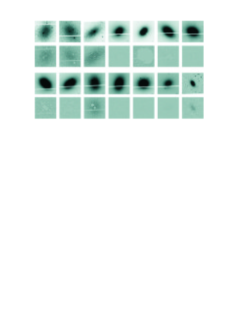
Figure 1: The original I-band images and residual frames. The object plotted are (from left to right, upper rows) DDO 71, KDG 61, KDG 64, NGC 474, NGC 1316, NGC 1344 and NGC 2865. Lower rows (left to right): NGC 3610, NGC 3923, NGC 5237, NGC 5982, NGC 7626, UGC 7369 and VCC 941. In the original frames a 10$\arcsec$ segment is also shown.

After sky and galaxy model have been subtracted, some large–scale deviations are present in the frame. We remove these deviations using the background map (BACK_SIZE parameter set to 25) obtained running SExtractor (Bertin & Arnouts, 1996) on the sky+galaxy subtracted frame. We will refer to this sky+galaxy+large–scale residuals subtracted frame as “residual frame”. ACS images of the 14 selected galaxies are shown in Figure 1, together with the residual frames.

We must emphasize that we succeeded in modeling the galaxy light with elliptical isophotes for all the selected galaxies, including the objects classified as irregular galaxies (Table A) and for the galaxies which show prominent shells. This was possible since $a$) the shells are prominent with respect to the smooth galaxy profile only in more external regions respect to the ones we considered for SBF and color measurements (Figure 1); $b$) the iterative modeling procedure provides a good model of the galaxy profile; $c$) the large scale residuals subtraction removes most of the large-scale (shell) features left behind by the modeling.

3.2 Sources Photometry

The next step in our procedure is to evaluate the photometric properties of point–like and extended external sources left in the image. The construction of the photometric catalog is critical for SBF measurement, as the estimation of the luminosity function of external sources is fundamental to properly evaluate the extra fluctuations due to the undetected sources present in the frame (Tonry et al., 1990).

The photometry of the sources is obtained independently on the I- and V-band frames using SExtractor, the output catalogs are then matched using a 0.1^′′ radius. Aperture corrections and extinction corrections are applied before transforming the ACS magnitudes into the standard I and V (C05).

The fit of the luminosity function is obtained assuming a gaussian Luminosity Function for the GC component (GCLF, Harris, 1991):

$$n_{GC}(m)=\frac{N_{0,GC}}{\sqrt{2\pi\sigma^{2}}}~{}~{}e^{-\frac{(m-m_{X,GC})^{2}}{2\sigma^{2}}},$$ (1)

plus a power-law luminosity function (Tyson, 1988) for the background galaxies:

$$n_{gxy}(m)=N_{0,gxy}10^{\gamma m},$$ (2)

where $N_{0,GC}$ ($N_{0,gxy}$, Blakeslee & Tonry, 1995) is the globular cluster (galaxy) surface density, and $m_{X,GC}$ is the X-band turnover magnitude of the GCLF at the galaxy distance. In expression (2) we used the $\gamma$ values obtained by Benítez et al. (2004). For the GCLF we assumed the turnover magnitude and the width of the gaussian function from Harris (2001), i.e -7.4 mag, -8.5 mag for the V- and I-band turnover magnitudes respectively, and dispersion $\sigma=1.4$ mag (see also §3.3). To fit the total LF we used the software developed for the SBF distance survey (T01) and optimized for our purposes; we refer the reader to C05 and references therein for a detailed description of the procedure. Briefly: a distance modulus ($\mu_{0}$) for the galaxy is adopted in order to derive a first estimation of $m_{X,GC}=\mu_{0}+M_{X,GC}$, then an iterative fitting process is started with the number density of galaxies and GC, and the galaxy distance allowed to vary until the best values of $N_{0,GC}$, $N_{0,gxy}$ and $m_{X,GC}$ are found via a maximum likelihood method.

The whole procedure of luminosity function fitting is not applied to DDO 71, KDG 61, KDG 64, and VCC 941. For these objects the few candidate globular clusters (if present) appear resolved in the ACS images, and are masked out. Similarly, the images of these galaxies allow us to recognize and mask out most of the brighter background galaxies (e.g. all sources brighter than 25th magnitude in the I-band), so that the contribution of the faint background galaxies is very small compared to the stellar fluctuations ($P_{r}/(P_{0}-P_{r})\equiv P_{r}/P_{f}$ $<$ 0.001, see Table 1 and next paragraph). As a consequence no extra–fluctuation correction has been applied to these galaxies.

3.3 SBF measurements

The pixel–to–pixel variance in the residual image has several contributors: ($i$) the poissonian fluctuation of the stellar counts (the signal we are interested in), ($ii$) the galaxy’s GC system, ($iii$) the background galaxies, and ($iv$) the photon and read out noise.

To analyze all such fluctuations left in the residual frame, it is useful to study the image power spectrum as all the sources of fluctuation are convolved with the instrumental PSF, except for the noise. We performed the Fourier analysis of the data with the IRAF/STSDAS task FOURIER.

In the Fourier domain the photon and read out noise are characterized by a white power spectrum, thus their contribution to the fluctuations can be easily recognized as the constant level at high wave numbers in the image power spectrum. On the other hand, since the stellar, globular clusters, and background galaxy fluctuation signals are all convolved with the PSF in the spatial domain, they multiply the PSF power spectrum in the Fourier domain. Thus, the total fluctuation amplitude can be determined as the factor to be multiplied to the PSF power spectrum to match the power spectrum of the residual frame.

The residual frame, divided by the square root of the galaxy model (Tonry et al., 1990), is fourier transformed and azimuthally averaged. The azimuthal average $P(k)$ is used to evaluate the constants $P_{0}$, and $P_{1}$ by fitting the expression:

$$P(k)=P_{0}\cdot E(k)+P_{1}\,,$$ (3)

where $P_{1}$ is the constant white noise contribution, $P_{0}$ is the PSF multiplicative factor that we are looking for, and $E(k)$ is the azimuthal average of the PSF power spectrum convolved with the mask power spectrum (Tonry et al., 1990). Since neither contemporary observations of isolated stars, nor good PSF candidates were available in our frames, we used the template PSFs from the ACS IDT, constructed from bright standard star observations.

As mentioned in the previous section, the fluctuation amplitude $P_{0}$ estimated so far includes stellar fluctuation and the contribution of unmasked external sources. To reduce the effect of this spurious signal, all the sources above a defined signal to noise level (typically we adopted a $S/N\sim 3.5$) have been masked out before evaluating the residual image power spectrum. Thus, at each radius from the galaxy center, a well defined faint cutoff magnitude ($m_{lim}$) fixes the magnitude of the faintest objects masked in that region. Such masking operation greatly reduces the contribution to $P_{0}$ due to the external sources, but the undetected faint and the unmasked low S/N objects could still affect $P_{0}$, thus their contribution – the residual variance $P_{r}$ – must be properly estimated and subtracted. The residual variance is computed evaluating the integral of the second moment of the luminosity function in the flux interval $[0,~{}f_{lim}]$:

$$\sigma_{r}^{2}=\int_{0}^{f_{lim}}N_{Obj}(f)f^{2}df$$ (4)

where $f_{lim}$ is the flux corresponding to $m_{lim}$, and $N_{Obj}(f)$ is the luminosity function previously obtained as the sum of the GCLF and the galaxies power law. The residual variance $P_{r}$ is then $\sigma_{r}^{2}$ normalized by the galaxy surface brightness. On average, the $P_{r}$ correction is small for all the galaxies. Thanks to the faint completeness limit of these images, it is typically $\sim$5% (7%) of the total fluctuations amplitude $P_{0}$ in the I (V) band frames, except for the dwarf galaxies for which no $P_{r}$ correction has been applied.

Finally, the SBF magnitude is obtained as follows:

$$\bar{m}_{X}=-2.5~{}\log(P_{0}-P_{r})+m_{zero}^{X,ACS}+2.5~{}\log(T)-A_{X}$$ (5)

where X refers to the I or V passband, $m_{zero}^{X,ACS}$ is the zeropoint ACS magnitude reported by S05 (VEGAMAG system), T is the exposure time, and A_X is the reddening correction.

Since we are also interested in studying the radial behavior of SBF, the procedure described above is applied to several distinct elliptical annuli for each galaxy; the annuli shape reflects the geometry of the isophotes profile.

Table 1 reports the final results of our measurements for each annulus and for all galaxies of the sample. Only annuli with SBF S/N$\geq$7 are taken into account (Jensen et al., 1996; Mei et al., 2001; Cantiello et al., 2007). The table columns give: (1) the average annular radius in $arcsec$; (2-3) the annulus color and uncertainty; (4-5) $P_{0}$ and $P_{r}$ for the V-band images ; (6-7) the V-band SBF magnitude; (8-9) $P_{0}$ and $P_{r}$ for the I-band images; (10-11) the I-band SBF magnitude. For each galaxy also the weighted average ($\langle av.\rangle_{w}$) color and SBF magnitudes are reported, when possible.

The quoted uncertainties are the statistical errors due to the sky estimations, and the PSF power spectrum fitting. A default $20\%$ uncertainty is associated to $P_{r}$ (Tonry et al., 1990; Cantiello et al., 2007), and included in the final SBF error. To test the robustness of the $P_{r}$ correction versus the sigma fitting parameter adopted for the GCLF, we have performed some tests by changing the sigmas in the range 0.8 to 1.6 (Jordán et al., 2006), as a result we find that the effect on the final SBF magnitudes is $<0.1$ mag in all cases. All uncertainties also include the error propagation of the color equations from Sirianni et al. (2005).

Additional systematic errors are $\sim$0.03 mag in the PSF normalization, $\sim$0.01 mag error from filter zeropoint, and $\sim$0.01 mag from the flat–fielding – see C05 for details.

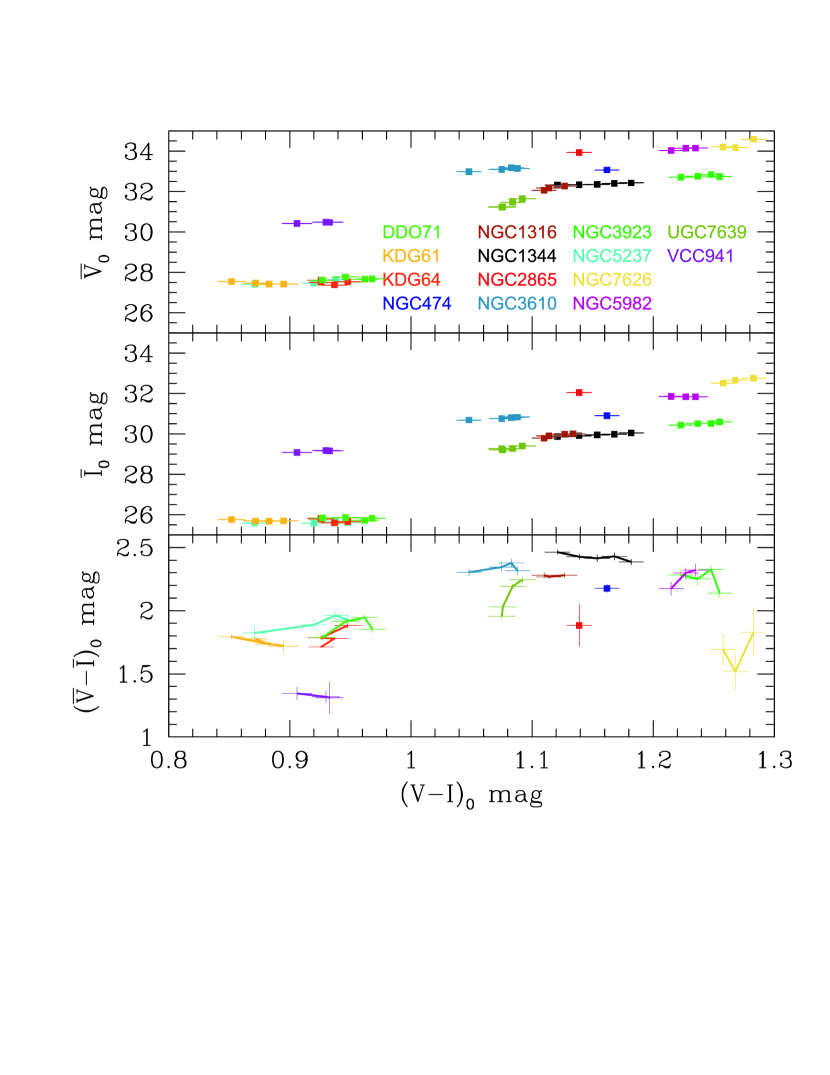
Figure 2: SBF apparent magnitudes and color versus integrated (V-I)₀ color. Different colors refer to different galaxies as labeled.

Figure 2 shows the V- and I-band SBF apparent magnitudes and the $(\bar{V}-\bar{I})_{0}$ annular data versus the annulus integrated color. As a first impression we see that, unlike our previous study (C05), no systematic SBF versus color gradient feature can be recognized. The presence of a SBF gradient has been estimated by fitting a least squares line to the I-band SBF and (V-I)₀ color data, and comparing the slope, $\alpha=\delta\bar{m}_{I}/\delta(V-I)_{0}$, with its uncertainty. Since, in all cases the change in color and $\bar{m}_{I}$ occurs as function of radius, we indicate in Table 1 as “SBF-gradient” those galaxies with slope $\alpha$ at least twice bigger than its estimated uncertainty (i.e. $\alpha/\Delta\alpha\geq 2$), the galaxies which do not fulfill this condition are labeled as “SBF-flat”.

4 Discussion

As mentioned before, the link between SBF amplitudes and stellar population properties lies at the base of the determination of the absolute SBF magnitudes for distances studies, via theoretical or empirical calibrations, and of the use of SBF to analyze the properties of the stellar populations in galaxies.

Taking advantage of the characteristics of our set of measurements, in the following sections we try to answer at two different questions. First, what can we infer in terms of stellar populations properties from SBF- and SBF-gradient versus color analysis? Second, given the number of calibrations available in literature, which one, applied to our measurements, gives the best results, i.e. distance moduli in agreement with the group distances reported in Table A?

4.1 Stellar population properties

4.1.1 Population properties from observational data

One major difference of the present data from most of the SBF works, is that the new dataset provides a sample of galaxies covering a wide range physical properties (total magnitude, morphological type); as a consequence we expect to find different stellar components to dominate the light emitted by these objects. Figure 3 shows a comparison of some galaxy’s physical quantities, from Table A, versus the average integrated color from Table 1. As readily apparent, large differences exist between the various objects, in particular the sample spans a range of 10 magnitudes in absolute B-band magnitude M_Bt.

By inspecting the panels of Figure 3, we note that the sample can be split in two subsamples: a blue subsample at (V-I)${}_{0}\leq 1.0$ mag, and a red subsample at (V-I)${}_{0}>1.0$ mag. The blue galaxies, with an average (V-I)${}_{0}\sim 0.92$ mag, are generally less luminous (M${}_{Bt}\sim-13.0\pm 1.1$) and cover a large range of morphological types. On the contrary, the red galaxies, at average (V-I)${}_{0}\sim 1.16$ mag, are brighter (M${}_{Bt}\sim-20.5\pm 1.8$), and morphologically more uniform.

Keeping in mind these points, in this section we take advantage of the SBF and color data reported in Table 1 to infer information on the physical properties of the dominant stellar system in the galaxies of our sample. We begin our comparisons by considering the average SBF measurements. Hence, only observational quantities are considered. We will introduce the comparison with models, and discuss the caveats of such discussion, later on.

As a first step, we plot the galaxy’s physical quantities used in Figure 3 against the SBF absolute magnitudes (Fig. 4, panels $a$ and $b$) as derived by assuming the distance modulus quoted in Table A. In the ($b$) panels the C05 data are also included. As a general result the plots disclose that SBF magnitudes show trends which are well consistent with what is found with integrated colors (Fig. 3). Clearly, the relationships are far from being well established due to the small number of galaxies in the sample. In spite of this, the $\bar{V}$ and $\bar{I}$ $versus$ M_Bt panels show a quite defined correlation.

For most of the blue galaxies, no H_β, Mg₂, or velocity dispersion $\sigma$ estimation is available from literature. However, taking into account the extrapolations shown by the dashed lines in the panels of Figure 3, these galaxies are also expected to have smaller Mg₂ and velocity dispersion, and higher H_β values with respect to the red counterpart. All these general properties agree with a scenario where the blue objects are low mass galaxies (low M_Bt and $\sigma$), with a relatively young/metal poor dominant stellar component (low Mg₂, high H_β), while the red objects are expected to be mostly massive galaxies populated by old, metal rich stellar systems – see for example Gallazzi et al. (2006) for a discussion based on a large sample of galaxies.

Somewhat more interesting are the correlations shown in the panels ($c$) of Figure 4, where we plot the same physical quantities as function of the SBF color. These measurements have the relevant feature of being distance-free. Contrary to the absolute SBF magnitudes, the SBF color shows little or no correlation with the plotted physical quantities. For example, the lower-left panel shows that $(\bar{V}-\bar{I})_{0}$ SBF color does not have a strong correlation with M_Bt absolute magnitude. This is expected on theoretical basis (e.g. Cantiello et al., 2003, §5.3), however this is the first time that such behavior is explicitly shown.

A further insight of these results is obtained when the presence or the absence of a radial SBF gradient is taken into account. The galaxies listed in Table 1 have been accordingly divided in two classes: $i)$ “SBF-gradient” galaxies are the ones showing a radial SBF gradient and $ii)$ “SBF-flat” galaxies which show nearly constant SBF magnitudes (within the uncertainties) over the explored annuli. The class $i)$/$ii$) is shown with full/empty squares in all the panels of Fig. 4. The SBF galaxies studied in C05 are also plotted in panels ($b$), with empty circles, to enlarge the present sample with 6 giant ellipticals, and a dwarf galaxy. All the galaxies of the C05 sample have a significant I-band SBF versus color gradient, with the only exception of the local dwarf NGC 404 (shown with an arrow in panels $b$).

Inspecting Figure 4, we find that the SBF-gradient galaxies tend to have fainter SBF magnitudes than SBF-flat galaxies, with VCC 941 being the only obvious exception to such behavior. More specifically, the average SBF absolute magnitudes are $\langle\bar{V}\rangle=-0.3\pm 0.1$, and $\langle\bar{I}\rangle=-2.1\pm 0.1$ for the SBF-flat objects, while they are $\langle\bar{V}\rangle=0.7\pm 0.2$, and $\langle\bar{I}\rangle=-1.5\pm 0.3$ for the SBF-gradient galaxies if the VCC 941 data are excluded. If also the absolute SBF magnitudes for this latter galaxy are taken into account, the differences between the SBF-flat and SBF-gradient galaxies are less evident but still recognizable, as we have $\langle\bar{V}\rangle=0.6\pm 0.5$ and $\langle\bar{I}\rangle=-1.5\pm 0.3$.

Since the presence or absence of a SBF gradient is related to the properties of the dominant stellar population, this feature could represent a relevant tracer of galaxy formation. As an example, as discussed in C05 (§4.2.1), the monolithic and hierarchical galaxy formation scenarios make opposite predictions on the radial behavior of the stellar population properties in a galaxy. In particular, in the hierarchical scenario of galaxy formation the radial differences of stellar population properties will flattens as galaxies undergo mergers. On the contrary, substantial radial gradients are expected if the galaxy formed following a pure monolithic collapse path (White, 1980; Bekki & Shioya, 2001, e.g.).

In conclusion, the analysis of the SBF radial gradients in galaxies might represent an interesting and innovative tool, to be used in parallel with other techniques, to study the history of galaxy assembly. SBF radial gradients are an observable physical quantity that can be analyzed and compared between galaxies, independent of the many model uncertainties. However, in order to constrain galaxy formation models using observed gradients, it is necessary to use models to go from observational quantities to physical properties. As will be shown in the next sections, currently the last step is very uncertain in some metallicity regimes. In this respect, new measurements are also necessary to enlarge the sample and to strengthen the use of SBF gradients as a tool to analyze galaxy formation.

As an additional way to examine such stellar population properties, SBF and color data can be compared to population synthesis models. In the following section we discuss the stellar population properties in our sample of galaxies by comparing data with model predictions.

4.1.2 Comparison with models and bias in the color transformations

In this section we derive and discuss the properties of the dominant stellar system in our sample of galaxies by comparing observations of SBF and integrated color data with SSP model predictions. At first we adopt the Teramo-SPoT models from R05 as the reference ones. We adopt these models as reference since they have proved to reproduce fairly well the Color–Magnitude Diagrams, integrated magnitudes and colors, and the SBF amplitudes both for star clusters (Galactic and Magellanic Clouds, MC, clusters), and for galaxies in the optical and near–IR passbands (Brocato et al., 2000; Cantiello et al., 2003, R05). We will also consider other sets of models later on in this section.

In Figure 5 we show the comparison of the average ($\bar{V}-\bar{I}$)₀ color and the absolute V- and I-band SBF magnitudes versus the galaxy color. The R05 models are shown for ages 3$\leq$ t (Gyr) $\leq$ 14, and metallicity 0.0003 $\leq Z\leq$ 0.04. In the Figure, models of equal metallicity are connected by dashed lines.

Taking into account the upper two panels in this Figure, a good match between models predictions and observational data is found, that is, the observational data generally overlap the grid of models, with the only exceptions of NGC 2865 and NGC 7626.

Even if the absolute magnitudes contain as additional uncertainty the distance modulus adopted, the relevant result in these panels is the good overlap between models and data, obtained for a wide range of observed galaxy colors, i.e. from 0.85$\ \raise-2.0pt\hbox{\hbox to0.0pt{\hbox{$\sim$}\hss}\raise 5.0pt\hbox{$<$}\ }(V-I)_{0}\ \raise-2.0pt\hbox{\hbox to0.0pt{\hbox{$\sim$}\hss}\raise 5.0pt\hbox{$<$}\ }$ 1.30. In this range, the observed $\bar{M}_{I}$ and $\bar{M}_{V}$ magnitudes decrease by moving from blue to red integrated colors. According to the R05 models shown in the figure, this means that the light emitted by blue-faint galaxies is dominated by metal poor stellar populations while red-bright galaxies are mostly populated by very metal rich stars.

SBF color data can be used to derive the two color SBF versus integrated diagram, which are independent of the distance modulus. By inspecting the lower panel in Figure 5 we find, as expected, that the observed SBF and integrated colors cover a large range of chemical compositions. In this panel, it can be recognized that the blue subpopulation, with an average $(\bar{V}-\bar{I})_{0}\sim 1.7\pm 0.2$ lies in the area of models with Z  $\sim$$<$ 0.001, possibly higher than 0.0001. The red subpopulation, at $(\bar{V}-\bar{I})_{0}\sim 2.2\pm 0.2$, seems more likely to be dominated by a Z  $\sim$$>$ Z_☉ stellar population. Moreover, while redder galaxies, at (V-I)${}_{0}>1.2$, are mostly located near the edge of old SSP models, the blue galaxies are spread over the whole age interval.

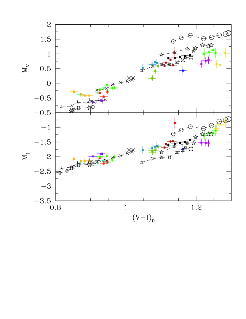
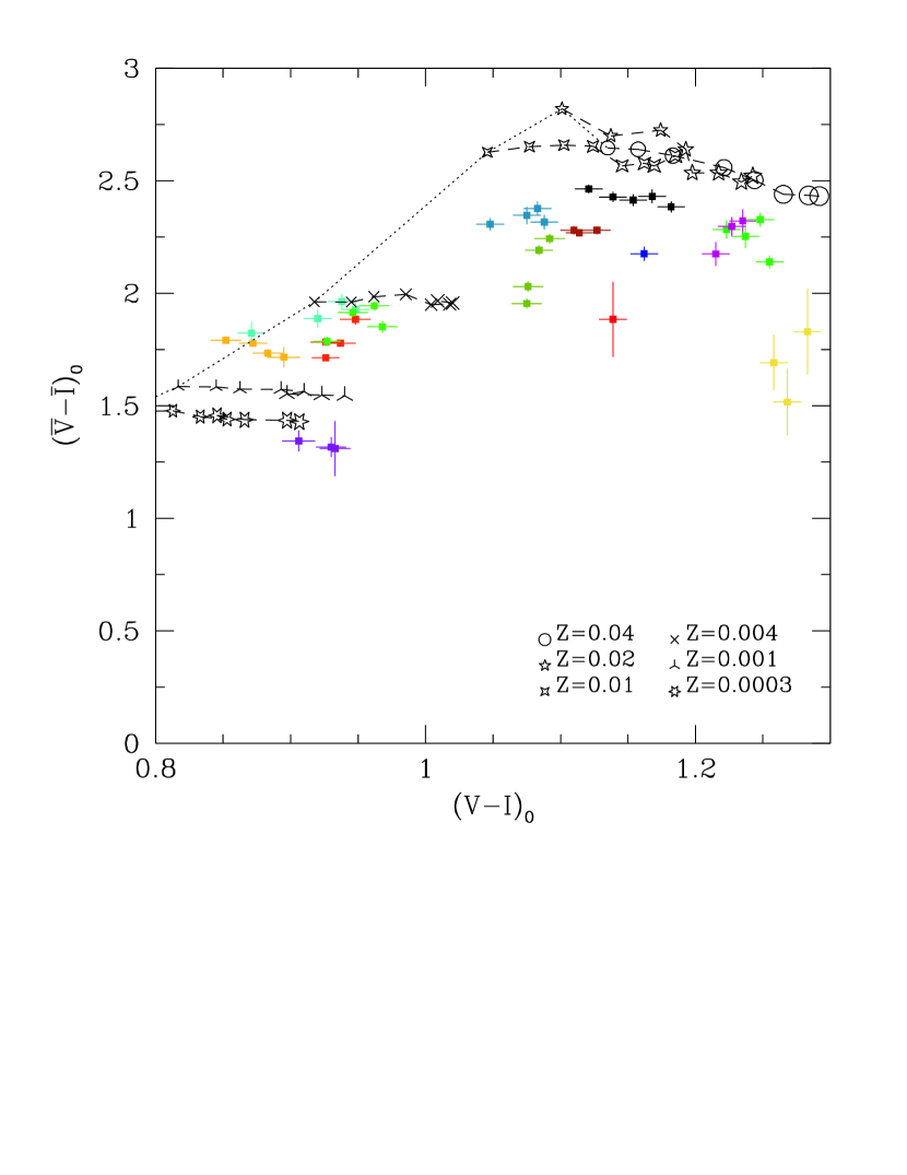
Figure 6: Left panels: Absolute SBF profiles versus the integrated (V-I)₀ color. Right panel: The distance free SBF-color versus integrated color panel. R05 models symbols are the same as in Figure 5. The dotted line connects the models at lowest ages, 3 Gyr, for all chemical compositions.

The drawback with the $(\bar{V}-\bar{I})_{0}$ color is that the models in the high metallicity regime are not well separated, leading to a highly uncertain data to models comparison. Note that such behavior is predicted by all recent SBF models, as will be shown in the following. In order to obtain more information from our SBF data, in what follows we will consider the single annulus SBF and color measurements for each galaxy, instead of the average values. This is done in Figure 6 where we compare the annular absolute SBF magnitudes and colors with R05 models. Again, the good matching of models with data in the $\bar{M}$ versus (V-I)₀ planes is encouraging, but we rather prefer to use the distance free SBF-color versus color data and models comparison to infer the properties of the stellar systems in the galaxy. Based on the content of the right panel in Figure 6, for each galaxy of our list we have obtained the age and chemical composition reported in Table 2 (see also the appendix for some more comments on individual galaxies).

First, we note that NGC 2865, and NGC 7626 data are noticeably far from the grid of models. In general, it can be argued that our measurements might suffer of the bias due to the ACS-to-standard magnitudes transformations. In fact, the observed SBF color range is redder than the range used by Sirianni et al. (2005) to derive their transformation equations. Furthermore, this bias could be stronger for the measurements obtained from F606W images due to the uncertainty of the F606W-to-V transformation – e.g. Figure 21 from Sirianni et al. (2005) shows that there is a non negligible difference between the F606W-to-V synthetic and empirical transformations. As a consequence, the V-band SBF data derived from F606W might be more uncertain than others.

Although the presence of some bias in our data cannot be ruled out, possible systematics can be highlighted by comparing these measurements with those available in literature, derived in standard V and I filters from ground based observations.

Blakeslee et al. (2001) obtained $(\bar{V}-\bar{I})_{0}=2.38\pm 0.11$, for a sample of galaxies in the Fornax cluster with M${}_{Bt}\leq-20.3$ mag. For the galaxies presented in this work we find that the SBF color for objects with M${}_{Bt}\leq-20.3$ mag is $(\bar{V}-\bar{I})_{0}=2.16\pm 0.23$, but it becomes $2.29\pm 0.08$ when NGC 2865, and NGC 7626 are excluded. If the latter number is taken into account, we can consider our measurements and the ones from Blakeslee et al. in good agreement. In addition, by comparing our measurements for NGC 1316 and NGC 1344 with those from Blakeslee et al. and T01, we find a good agreement for NGC 1316, while for NGC 1344, that is one of the F606W-to-V SBF measurements, the measurements still agree with each other, but to a lower degree.

The whole sample of objects with contemporary V and I SBF measurements from the literature is shown in Figure 7, together with our measurements. In this figure, the $(\bar{V}-\bar{I})_{0}$ data are compared with the Mg₂ index and the central velocity dispersion (both data from Leda). The GC data shown in the figure come from Ajhar & Tonry (1994), and R05, the galaxies data are from Blakeslee et al. (2001), Tonry et al. (1990), Tonry & Schechter (1990), and this work. As mentioned above, by inspecting this Figure we find that, if NGC 2865, and NGC 7626 are excluded, the data presented in this work do not show any peculiar behavior with respect to other (galaxies) data.

Moreover, comparing the left panel of Figure 7 with the Figures 14 and 15 from Ajhar & Tonry (1994), we find that the only “unusual” galaxy is NGC 2865. More in detail, as discussed by Ajhar & Tonry (1994), there is a continuous trend in $(\bar{V}-\bar{I})_{0}$ versus Mg₂ from GC up to bright galaxies, but there seems to be a wide spread when Mg₂ reaches $\ \raise-2.0pt\hbox{\hbox to0.0pt{\hbox{$\sim$}\hss}\raise 5.0pt\hbox{$>$}\ }0.3$. Ajhar & Tonry (1994) argued that this could be due to the behavior of the giant branch with metallicity, as the “Mg₂ saturates before demonstrating the entire behavior of $(\bar{V}-\bar{I})_{0}$”. In particular, the different saturation limits of the blanketing with the metallicity in the V and I bands, might cause the $\bar{V}$ to reach a saturation minimum brightness, while the $\bar{I}$ still gets fainter at increasing metallicity. The location of NGC 7626 (and NGC 4365, from the Tonry et al. (1990) sample) in the panels of Figure 7 seems to confirm such behavior.

In other words, although our measurements could be affected at some degree by the presence of a bias due to the ACS to standard magnitudes transformations, the comparison of the present data with the data from literature seems to exclude the presence of an overall bias effect. Moreover, the unusual blue SBF color for NGC 7626 could be related to a differential metallicity saturation effect already discussed by Ajhar & Tonry (1994). On the other hand, the behavior of NGC 2865 still appears peculiar with respect to the whole set of data shown in Figure 7, possibly related to a bias in the data (e.g. transformations), or to intrinsic properties of this galaxy (e.g. dust, young stellar systems), or both.

A second consideration is that, using the R05 models, the model predictions are generally confined to a narrow range of chemical compositions for each galaxy, while the age limits are defined only in few cases (e.g. VCC 941). In the appendix, for each galaxy of our list we quote the stellar properties derived using other indicators; however, to further check the general age and metallicity values obtained, here we compare our estimations with other age/metallicity sensitive properties.

Concerning the chemical compositions, in Figure 8 the upper and lower bounds of the metallicity estimations drawn from the models comparison are plotted against the metallicity sensitive index $Mg_{2}$ (panel $a$), and with the total absolute magnitude M_Bt of the galaxy (panel $b$). From these panels we can recognize the correlation of the Mg₂ index with metallicity, and the metallicity-luminosity relation. More specifically, it is confirmed that the light from the blue sample of galaxies is dominated by a more metal poor stellar component with respect to the red subsample.

We have additionally compared our age estimations with the age sensitive index $H_{\beta}$. In this case, no significant correlation emerges. However, it is worth noting that the $H_{\beta}$ measurements are confined to very small radii.

These findings should be considered as encouraging results in the sense that they confirm the use of SBF magnitudes, color and gradients as a valuable stellar population tracer mostly sensitive to the chemical content of the galaxy.

One final comment, for the R05 models, is that the two-color diagram in Figure 6 shows that the SBF color of red galaxies is not well reproduced by models, with SBF color predictions systematically $\sim 0.2$ mag redder than the observed ones. Moreover, one could argue that the validity of stellar population properties presented in this section is strictly model dependent. To encompass such evidence, and test the robustness of predictions against models systematics, let us we take into account several other recent SBF models derived from SSP simulations.

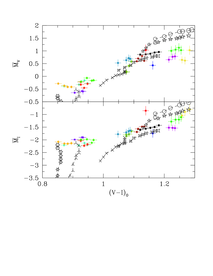
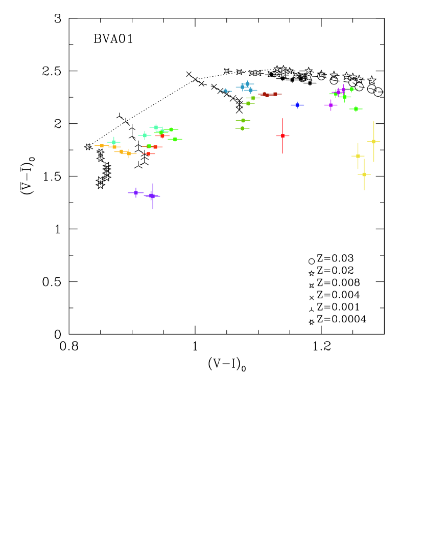
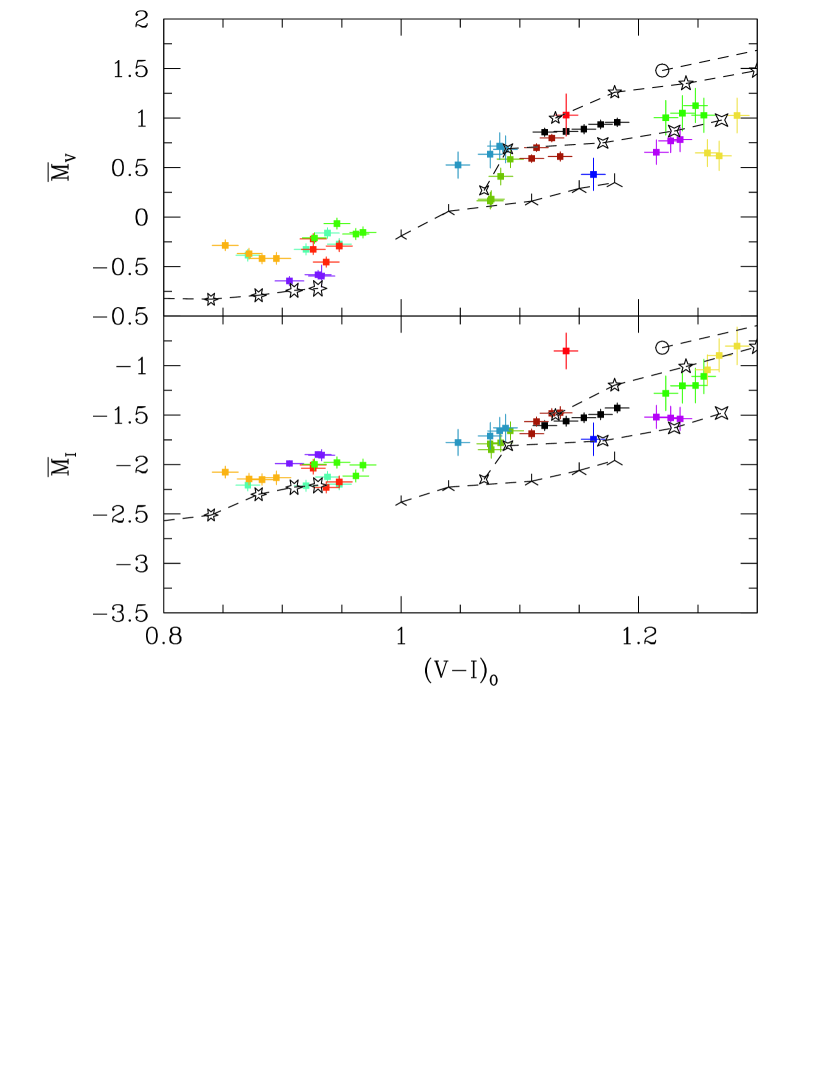
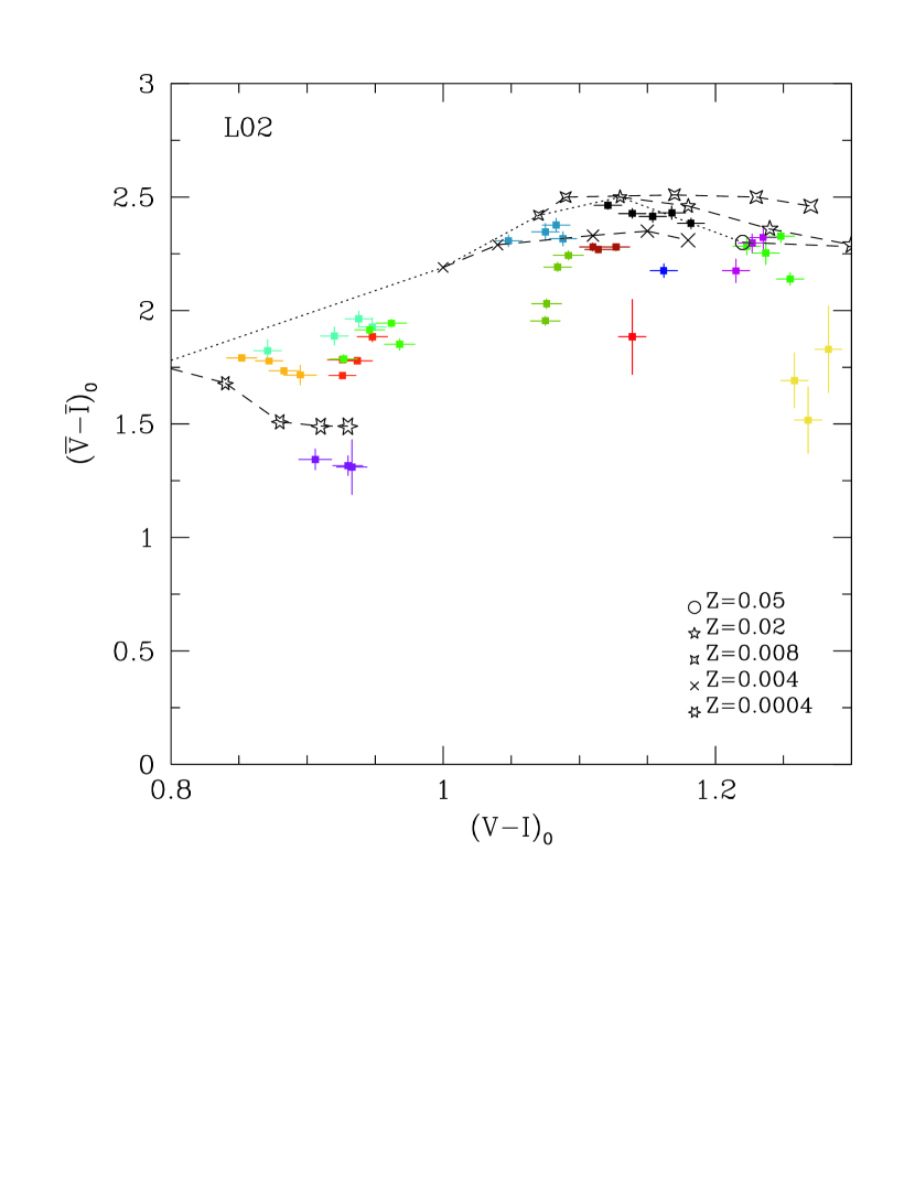
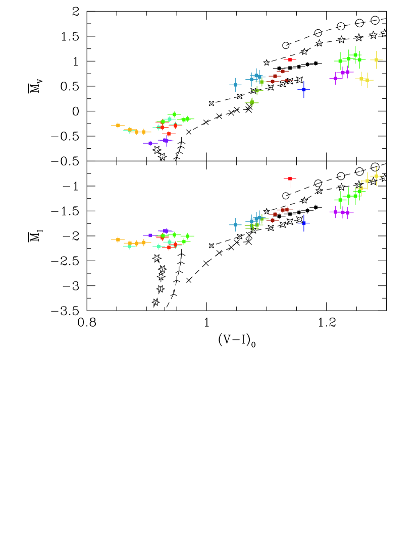
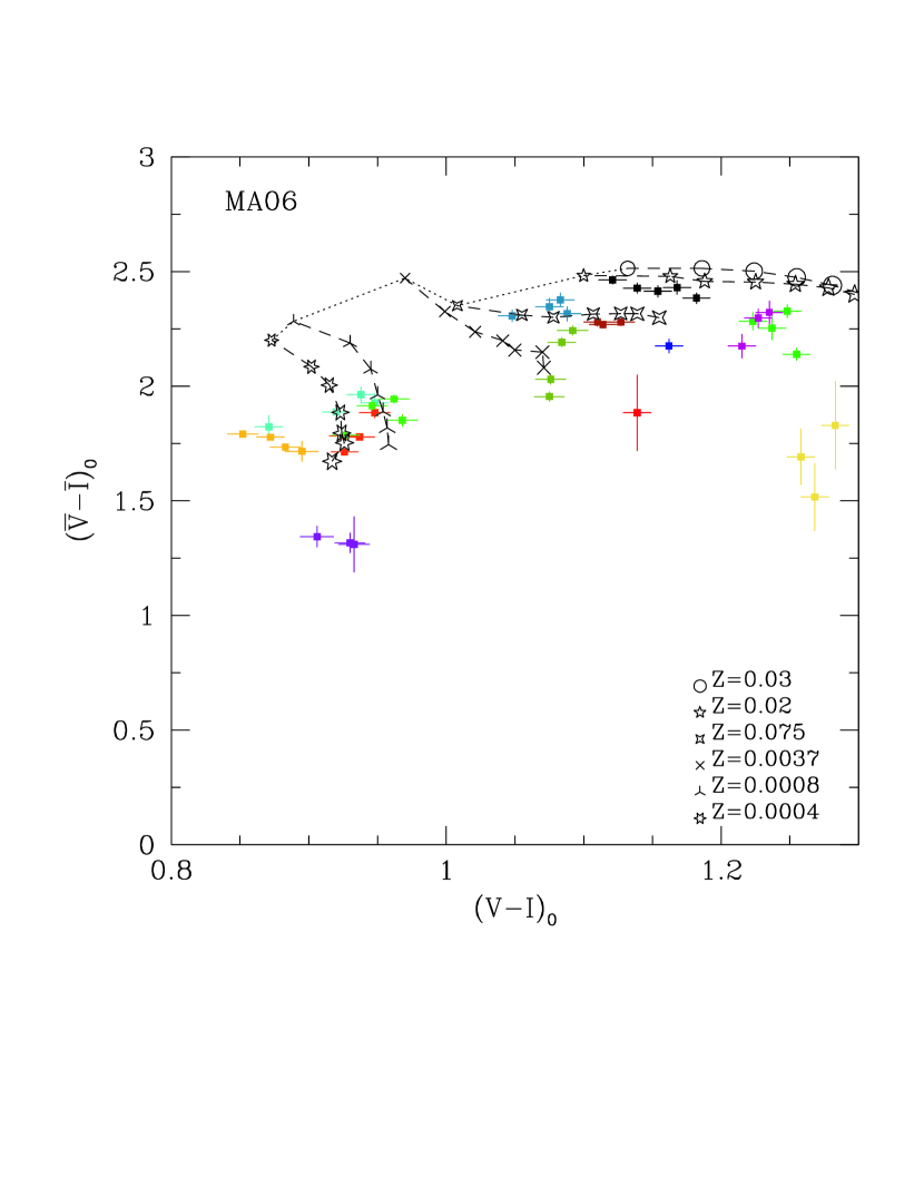
Figure 9: As Figure 6 but for the BVA01 (upper panels), L02 (middle), and MA06 models (lower panels). The age range is t=5 to t=17.8 Gyr (step of 12%) for BVA01; t=3,5,8,12,17 Gyr for L02 models; t=3,5,7,9,11,13,15 Gyr for MA06 models. The dotted lines connect models at 5, 3, and 3 Gyr for the three models, respectively.

In Figure 9 we show the same comparison presented in Figure 6, but for the Blakeslee et al. (2001), Liu et al. (2002), and Marín-Franch & Aparicio (2006) (BVA01, L02, and MA06 respectively hereafter) stellar population models.

As a first comment, we notice that at the high metallicity regime (Z  $\sim$$>$ 0.01) the SBF magnitudes versus (V-I)₀ color behavior is quite similar for all models. This is probably due also to the fact that the topology of the grid of models here can be very complex, leading to high degeneracy. On the other side the slight mismatch for the red galaxies noted with the R05 models is still present in these other sets of models. As suggested by BVA01, this could be due to the use of SSP models, while composite stellar populations would be more appropriate. Additionally, we mention that in most of the red galaxies SBF gradients (i.e. stellar populations gradients) have been found. Moreover, it must be noted the non–negligible differences between the various models in the low-Z regime.

Keeping in mind such limits of SSP models, we have analyzed the location of each galaxy in the SBF-color versus color plane with respect to models in order to derive the stellar population properties, as for the R05 models. The results are reported in Col. 3-5 of Table 2 (see also appendix). As can be recognized from the data in the Table, the chemical composition ranges obtained with the different models show a general good overlap.

On the other hand, we find that the ranges of acceptable ages are quite large, similarly to what obtained with R05 models. Thus, a robust conclusion of this work is that SBF can provide, given the current stage of the models, reliable estimates of the typical metallicities of galaxies, while the age of the dominant stellar system cannot be well constrained with this technique.

The right panel of Figure 8 shows the metallicity versus Mg₂ and M_Bt comparisons already discussed for the R05 models, except that in this case the average metallicity from the four different models is considered. The [Fe/H]–Mg₂ correlation is still present, although the data refer only to the red sample of galaxies. The relationship between [Fe/H] and M_Bt is more interesting. In fact, a mean least–squares fit to the data shown in Figure 8 (panel $d$) yields: [Fe/H]$\sim$ (-0.12 $\pm$ 0.02) $\times$ M_Bt - (2.8 $\pm$ 0.3). The agreement of this equation with similar relations existing in literature (e.g. Kobulnicky & Zaritsky, 1999; Contini et al., 2002) leads us to conclude that, within the limits of the present treatment, the method proposed provides us with reliable ranges of acceptable metallicities. Therefore, the metallicity properties derived from models can be considered by and large acceptable. Once again, no noteworthy correlation of ages with the H_β index is recognizable.

Let us now look more in detail to the model predictions for the single galaxies. Doing such comparison, consistent results with different models would imply a significant constraint on the properties of the stellar system observed, on the other hand a lack of agreement between models will possibly highlight uncertainties in the theoretical predictions.

Inspecting single galaxies it can be seen that at high metallicity (Z  $\sim$$>$  0.01) the differences between model predictions are less severe with respect to the case of Z  $\sim$$<$ 0.001. More in detail, the L02 and R05 models predict that age variations in the low metallicity regime do not affect the SBF color, while integrated colors suffer a noticeable change. On the contrary, BVA01 and MA06 models predict almost constant integrated colors at different ages, and a substantial SBF color variation.

The differences at low metallicity are possibly originated by a different treatment of the evolutionary properties of the bright, cold stellar component along the RGB and AGB in the various models. Until such discrepancies are resolved, little can be said about the origins of SBF gradients in this metallicity regime. However, such differences are interesting for the purpose of refining the models for the evolution of RGB and AGB stars. As well known, in fact, the SBF magnitude at these wavelengths is very sensitive to the properties of RGB/AGB stars, which suffer from large uncertainties, e.g. in atmosphere models, mass loss and stellar wind. In the optical regime, at lower metallicities the giant branch is brighter with respect to higher metallicities, thus it has a stronger effect on the luminosity weighted SBF signal. As a consequence, the discrepancies between various models in the treatment of the bright RGB/AGB phases appear more clearly in the SBF models at the low Z regime. Adopting this view, the disagreement between models can be solved by refining the modeling of the evolutionary properties of giant branch stars. Or, viceversa, coupling the bright star sensitive SBF color and integrated color data with metallicity and age information from independent indicators, would provide information useful to the challenge of a refined modeling of RGB/AGB stars.

4.1.3 SBF gradients and models

In addition to the above considerations, we now discuss the gradients of stellar populations properties, also taking advantage of some C05 results. As noted before, differently from C05 where we succeeded in revealing the systematic presence of SBF gradients in seven elliptical galaxies over eight, in our new sample of data we do not find a systematic presence of SBF gradients.

Before going on with the discussion of the gradients we must emphasize that such discussion, as for the results presented in the previous sections, is highly model–dependent. However, in contrast to the previous comparisons, where we compared observations with absolute values of SBF and colors, here we are only considering the slopes of such SBF versus color relations. On the other hand, it is easy to recognize that the slopes of the SBF versus (V-I)₀ relations can change quite a lot depending on the models. For example, if one considers the slope $\delta\bar{M}_{I}/\delta(V-I)_{0}$ at fixed Z, it has an average value of 3.3 for the R05 models, but it can be as high as $\delta\bar{M}_{I}/\delta(V-I)_{0}=14.3$ if the BVA01 models are considered. As explained before this is mostly due to the strong differences between models at the low metallicity regime. If only models at $Z\ \raise-2.0pt\hbox{\hbox to0.0pt{\hbox{$\sim$}\hss}\raise 5.0pt\hbox{$>$}\ }0.01$ are considered, in fact, such differences disappear, as we find that $\delta\bar{M}_{I}/\delta(V-I)_{0}$ at fixed metallicity lies in the range of 3.2-4.5 for all the models. At the same time the $\delta\bar{M}_{I}/\delta(V-I)_{0}$ at fixed age lies in the range 7.3-9.7, in good agreement for all the models at $Z\ \raise-2.0pt\hbox{\hbox to0.0pt{\hbox{$\sim$}\hss}\raise 5.0pt\hbox{$>$}\ }0.01$.

These numbers tell us that any obvious SBF-gradient in the low metallicity regime cannot be interpreted clearly as age–driven or metallicity–driven gradients, because of the differences between models. On the contrary, in the high-Z regime all models predict that a gradient related to pure age variations has a SBF versus color slope one half the slope of a gradient due to pure age variations. Obviously, real galaxies do not follow the simple scheme of “pure age(metallicity) radial variations”, however, as done in the previous sections, our observational data can be used to set some constraints at least to the effective dominant stellar system in the galaxy. Keeping in mind these limits, let us make some considerations on the SBF-gradients for the galaxies located in the area of high-Z models.

In C05, we have found that the gradients were mainly explained by metallicity variations within the galaxy, the inner regions being more metal rich than the outer ones. In the new sample we find that in the cases where a stellar population gradient is evident (SBF-gradient galaxies in Table 1), it is mostly explained by a age gradient rather than by a metallicity one. For example, this is the case of NGC 1344, where $\alpha\equiv\delta\bar{m}_{I}/\delta(V-I)_{0}=2.8\pm 0.3$. However, in few cases (e.g., UGC 7369 where $\alpha=9.0\pm 3.2$) a metallicity gradient is probably observed, no matter what set of models is considered.

For the galaxies in the low-Z regime, as already mentioned, the diversity between models hampers any clear justification of the source of the gradient itself, and different models predict opposite explanations to the presence of the gradient.

The differences between the present results and those by C05 can be ascribed to the sample selection. In fact, the list of objects taken into account in this work covers a wider range galaxy properties with respect to the C05 sample, which is mostly limited to massive ellipticals. In C05, the only exceptions to the uniform SBF gradient behavior were NGC 1344 and NGC 404, that is the galaxies with the lowest mass in the sample. For NGC 1344 an age–driven gradient was predicted, as also confirmed by the SBF color measurements in this work; while for the local dwarf galaxy NGC 404 no sign of evident age or chemical composition gradient was recognized, as it is the case for almost all the present dwarf galaxies.

By coupling the data in this work, with the results from C05 we are lead to the general indication that normal/bright ellipticals preferentially show a metallicity gradient, with the inner galactic regions being more metal rich with respect to the outer ones.

On the other hand, we have found that in some galaxies it is very likely that the observed gradient is probably due to a radial change of age, although the absolute age estimation is not feasible using available models. Most of such galaxies, like NGC 1344, show evidence of morphological irregularities indicative of recent merging activity.

Finally, the less massive objects invariably show no evident signs of SBF-gradients, or, as in the case of VCC 941, the gradient cannot be obviously interpreted in terms of metallicity or age variation effects, because of the disagreement existing between different models in this metallicity regime.

In conclusion, our SBF color versus integrated color study seems to point out that there is a metal enrichment in the stellar populations at inner galaxy regions, and that such behavior is related to the galaxy mass, as it can only be recognized in the more massive objects. The possible age–driven gradients, also observed in our sample, are mostly related to specific environmental properties (e.g. galaxy interactions).

Before closing this section, we say a few words about the consequences of the metallicity properties derived above on the RGB Tip distances. All the galaxies of the blue subsample, in fact, come from proposals designed to derive RGB Tip distances of the target galaxy. By using the R05 models we find that for all the galaxies at (V-I)${}_{0}\ \raise-2.0pt\hbox{\hbox to0.0pt{\hbox{$\sim$}\hss}\raise 5.0pt\hbox{$<$}\ }1$, the age and chemical compositions limits given above imply a RGB Tip magnitude in the I-band which is practically constant for the whole intervals quoted, i.e. $M_{I,RGBTip}\sim-4.2$ mag. The model predictions are slightly brighter with respect to the observational RGB Tip magnitudes adopted by Karachentsev et al. (2006), which use $M_{I,RGBTip}\sim-4.05$ mag. However, we must mention that $i$) both the theoretical and observational data agree within uncertainties; $ii$) the light of galaxies at (V-I)${}_{0}\ \raise-2.0pt\hbox{\hbox to0.0pt{\hbox{$\sim$}\hss}\raise 5.0pt\hbox{$<$}\ }1$ is expected to be dominated by a metal poor (Z  $\sim$$<$ 0.001) stellar system, thus brighter RGB Tip magnitudes are expected (e.g. Salaris & Cassisi, 1998); and that $iii$) the theoretical predictions do fully agree with the recent calibration from Rizzi et al. (2007). Adopting the above theoretical calibration implies an average of 8% higher distances with respect to the one adopted by Karachentsev et al. (2006).

4.2 Determining the best $\bar{M}$ versus (V-I)₀ calibration

Since the first appearance of the SBF method, a few different calibrations of the $\bar{M}_{I}$ absolute SBF magnitude versus the (V-I)₀ color have been introduced, by using either observations, or theoretical models. In this section we focus our attention on empirical calibrations reviewing the most recent ones . Typically such equations are derived from different observational data, and they are valid only within the range of colors of the defining sample, which is basically narrower than the color range of the present sample. We apply these calibrations to our set of measurements and compare the distance moduli so derived $\mu_{0,cal}$ with the group ones $\mu_{0,group}$ obtained from literature data (Table A). The minimization of the $\Delta\mu_{0}=\mu_{0,cal}-\mu_{0,group}$ versus the calibration equations, will enable us to identify the best empirical calibration in the color interval 0.85$\ \raise-2.0pt\hbox{\hbox to0.0pt{\hbox{$\sim$}\hss}\raise 5.0pt\hbox{$<$}\ }(V-I)_{0}\ \raise-2.0pt\hbox{\hbox to0.0pt{\hbox{$\sim$}\hss}\raise 5.0pt\hbox{$<$}\ }$ 1.30. For this study we use the average SBF and color measurements from Table 1.

Among the few available, we will consider the following calibrations:

$$\bar{M}_{I,T01}=-1.74\pm 0.08+(4.5\pm 0.25)[(V-I)_{0}-1.15]$$ (6)

from T01, obtained using a sample of $\sim$ 300 galaxies in different groups, zeropoint magnitude calibrated using the $HST$ Key Project Cepheids distances by Ferrarese et al. (2000b).

Then we consider the other:

$$\bar{M}_{I,J03}=-1.58\pm 0.08+(4.5\pm 0.25)[(V-I)_{0}-1.15]$$ (7)

from Jensen et al. (2003), which is essentially the same as the Eq. 6, but the zeropoint is derived using the revised $HST$ Key Project Cepheid distances from Freedman et al. (2001), without the metallicity correction. Both equations are valid in the range of color 0.95 $\leq$ (V-I)${}_{0}\leq$ 1.30.

In combination with these equations, for those objects at (V-I)${}_{0}\leq 1.00$ we apply the calibration derived by Ajhar & Tonry (1994) from globular clusters, upgraded by using the most recent distances and extinctions from the Harris (1996) catalog, including also the measurements for old (t  $\sim$$>$  10 Gyr) LMC globular clusters from R05. With all these upgrades we obtain:

$$\bar{M}_{I}=2.17\pm 0.27$$ (8)

using the star clusters with (V-I)${}_{0}\leq 1.00$.

Finally, we also take into account the recent calibration from Mieske et al. (2006), derived from Fornax cluster galaxies, in the color range 0.85 $\leq$ (V-I)${}_{0}\leq$ 1.10:

$$\bar{M}_{I,M06}=-2.13\pm 0.17+(2.44\pm 1.94)[(V-I)_{0}-1.00],$$ (9)

we coupled this equation with Eq. 7 for galaxies at (V-I)${}_{0}>$ 1.10.

The calibration from Ferrarese et al. (2000b) is not considered here as it agrees within uncertainties with Eq. 6. These authors, in fact, using a similar approach to T01, adopted the same slope of Eq. 6, but found a zero point of -1.79 $\pm$ 0.09 mag.

In Table 3 we show the distance moduli obtained adopting the above calibrations. In the Table we also show the group distance modulus for each object, which is used to derive the reduced $\chi^{2}$, and the average differences $\Delta\mu_{0}\equiv\langle\mu_{0,cal}-\mu_{0,group}\rangle$. Both the quantities $\chi^{2}$ and $\Delta\mu_{0}$ are reported in the last rows of the Table.

As shown by the numbers in the last two rows of Table 3, the best matching with the group distances is obtained coupling equation 7 with the 8, namely:

$$\bar{M}_{I}=-1.58\pm 0.08+(4.5\pm 0.25)\times[(V-I)_{0}-1.15],~{}~{}~{}~{}1.00<(V-I)_{0}\leq 1.30$$ (10)

$$\bar{M}_{I}=-2.17\pm 0.27,~{}~{}~{}~{}0.80<(V-I)_{0}\leq 1.00.$$ (11)

We note that if we apply the latter equations to the SBF measurements for 25 Fornax Cluster galaxies from Mieske et al. (2006), a median distance modulus 31.3 $\pm$ 0.4 is obtained, which is consistent with the expected group distance for this cluster $\mu_{0}\sim$31.5.

As an additional check, we have carried out for our V-band measurements the same analysis performed on I-band calibrations. The main difference in this case is that there is one only recent empirical calibration, from BVA01. These authors provide:

$$\bar{M}_{V,BVA01}=0.81\pm 0.12+(5.3\pm 0.8)[(V-I)_{0}-1.15].$$ (12)

Although this equation has been derived using data in a narrow range of colors (1.05$\leq(V-I)_{0}\leq$ 1.25), we tentatively extend its validity to the same range of Eq. (10) colors – such assumption is not completely arbitrary: in fact, as shown by numerical simulations, at fixed age the V-band SBF magnitudes have a more linear behavior versus $(V-I)_{0}$ respect to the I-band (e.g., Figures 6-9, and Figure 5 in Cantiello et al., 2003). We have renormalized the BVA01 zeropoint using the same criteria adopted by Jensen et al. (2003).

Again, for the blue galaxies we adopt the calibration derived from globular clusters using the Ajhar & Tonry (1994) and R05 measurements. In this case we obtain:

$$\bar{M}_{V}=-0.50\pm 0.27.$$ (13)

Coupling the latter two equations with our SBF and color measurements, we obtained the distance moduli also reported in Table 3 (Col. 7).

Using the best I- and V-band calibrations (Eqs. 10-11, and 12-13, respectively) we obtain the weighted average distance moduli reported in the last column Table 3. Once more, we note that the general validity of the calibrations is shown by the satisfactory agreement between the distance moduli derived and the group distance moduli.

As an aside, we also derived an independent calibration for the $\bar{M}_{V}$ versus (V-I)₀ equation, coupling our measurements with other data from literature. As a result we have found that the calibration obtained agrees within uncertainties with Eq. 12-13 in the whole range of $(V-I)_{0}$ colors considered here.

Before concluding this section we point out three facts. First, Karachentsev et al. (2006) obtained a distance modulus $\mu_{0}=30.32$ for UGC 7369, based on the RGB Tip method. However, they also state that this galaxy “does not look to be a nearby object”, and that it is “plausible association with the Coma I group” at a distance modulus 31.07 $\pm$ 0.07 (T01). As shown by the data in Table 3 our SBF measurements support this last hypothesis.

Second, it has been widely discussed by Richtler (2003) that the Globular Cluster Luminosity Function (GCLF) is a quite reliable distance indicator, although some exceptions exist. In his review, Richtler uses the SBF distances from T01 to derive the GCLF absolute Turn Over Magnitude (TOM). One of the main exceptions to the universality of the GCLF is NGC 3610, whose TOM is $\sim$ 2 magnitudes fainter than expected. Richtler argues that one of the possible causes of such mismatch is the presence of a population of intermediate-age metal-rich clusters, resulting in a fainter TOM. However, even though only the blue subpopulation of clusters is taken into account, there is still a large offset between NGC 3610 and the other galaxies. We find worth noting that, in their recent study on the GC system of NGC 3610, Goudfrooij et al. (2007) have found $M_{V}^{TOM}\sim-7.2$ mag. However, these authors erroneously state that they adopt a “distance modulus of $(m-M)_{0}=32.65$ as measured from T01”. The distance modulus quoted for this galaxy by T01, in fact, is 31.65 $\pm$ 0.22, which leads to $M_{V}^{TOM}\sim-6.2$, one magnitude fainter than the typical value for normal elliptical galaxies.

On the other hand, if we adopt the average distance modulus of NGC 3610 from Table 3, $\mu_{Ave}=32.71\pm 0.08$, and the blue clusters TOM 25.44$\pm$0.10 from Whitmore et al. (2002), the absolute TOM is $M_{V}^{TOM}=-7.27\pm 0.13$, in good agreement with the universal TOM from Richtler $M_{V}^{TOM}=-7.35\pm 0.24$. The difference between our distance and the estimation from T01 is probably due to the much lower quality of the NGC 3610 ground-based data used by T01, compared to these high resolution ACS images. Inspecting the data quality flags from T01 (see their Table 1, Q and PD values), we find that the SBF magnitude of NGC 3610 should be considered as poorly constrained. Moreover, the T01 distance of the other galaxy NGC 3613, which is classified as same group member of NGC 3610, agrees within uncertainties with our new SBF distance.

Finally, by using the average distance moduli in the last column of Table 3, and the $v_{flow}$ values reported in Table A, we obtain $H_{0}\sim 71\pm 14$ km s^-1 Mpc^-1, if the galaxies with $v_{flow}\ \raise-2.0pt\hbox{\hbox to0.0pt{\hbox{$\sim$}\hss}\raise 5.0pt\hbox{$>$}\ }~{}1000~{}km/s$ are taken into account.

5 Conclusions

The SBF and color properties obtained from ACS V- and I-band images of 14 galaxies have been discussed. The data were drawn from the HST archive. Classical integrated and SBF magnitudes have been derived using the standard analysis procedures. Our set of measurements is unique in terms of the wide range of $(V-I)_{0}$ color. We have taken advantage of this property to address different questions concerning both the use of SBF measurements as a distance indicator, and as a stellar population tracer.

With regard to the use of SBF to study stellar populations issues, we have analyzed the properties of the dominant stellar population in the selected galaxies by coupling V- and I-band SBF magnitudes with the $(V-I)_{0}$ color of the galaxies. As expected the list of objects covers a wide range of stellar populations properties. Since the outcome of this study depends on the set of population synthesis models adopted, we have taken into account different models to test the robustness of the predictions against the models systematics. Different sets of SSP models typically provide chemical composition estimations similar to each other and to our reference R05 models. However, from this comparison we have found that generally it is not possible to derive reliable age constraints for the stellar component in each galaxy, due to the non–negligible differences between models, especially at lower metallicities. In other words, multi–models comparison has shown that this technique is not efficient to strongly constrain the age for old (t  $\sim$$>$ 3 Gyr) stellar systems, but it can realistically be used to confine the metallicity range of the stellar system that dominates the light emitted by the galaxy.

These results confirm the usefulness of this kind of analysis to investigate the evolutionary properties of the unresolved stellar component in distant galaxies. On the other hand – where model differences arise – they also indicate that the present knowledge of stellar evolution, with particular regard to the properties of cool, bright giant branch stars, is still an open question which could be efficiently challenged taking advantage of SBF color data.

We have also examined radial SBF behavior for the sample of 14 galaxies. Comparing the gradients with models, and taking also into account the results from C05, we observe that usually the dwarf galaxies do not show substantial SBF gradients, thus we do not find any sign of systematic radial age/metallicity variation. Moreover, where such gradients are observed (e.g. VCC 941) the opposite predictions made by different sets of models make it difficult to understand if such gradients are related to radial changes of age or metallicity. On the contrary, for more massive objects a preferential metallicity driven gradient is noticed, with the outer galaxy regions being more metal poor than the inner ones. Possible age gradients have also been found, however they are usually related to a recent merging event. As a consequence, our SBF gradient data seem to point out the existence of a mass–related metallicity gradient in spheroidal galaxies. Given the connection between the gradients of stellar populations properties (i.e. SBF- and color-gradients) and the possible galaxy formation scenarios, we suggest that a future, enlarged database of SBF gradient data will also provide a valuable tool to trace the history of galaxy formation.

In conclusion, our study illustrates the potential of a study of galaxy properties based on the comparison of SBF colors with populations synthesis predictions. The current state of SBF models allows for a robust determination of the mean metallicities of galaxies, and an improved understanding of the stellar evolution phases important for SBF might allow the use of SBF in the future for detailed population studies. As in Cantiello et al. (2003), again we remark that multi–wavelength SBF data involving optical to near–IR observations are of paramount interest to push forward this technique. As shown by model predictions, indeed, SBF colors like $\bar{B}-\bar{K}$ are not affected by the models degeneracy shown by the $\bar{V}-\bar{I}$ color. Additionally, such color data are sensitive to stars in different phases of their evolution – e.g., $\bar{B}$ to Horizontal Branch stars, $\bar{K}$ to Thermally–Pulsing AGB stars – and are expected to be much more efficient to trace the stellar content of the galaxy, that is to trace back the history of galaxy formation.

Concerning distance studies, to check the validity of some I-band (and V-band) empirical calibrations existing in literature, we have estimated the galaxy distance moduli coupling our data with the various empirical calibrations. Then, these distance moduli have been compared with group distances derived from literature. We have found that the best I-band calibration is obtained matching two relations: $a$) in the range 1.00$<(V-I)_{0}\leq$1.30 the equation by Jensen et al. (2003), which is basically the one obtained by T01 with a different (fainter) zeropoint; $b$) for the range of color 0.80$\leq(V-I)_{0}\leq$1.00, a constant absolute magnitude, derived from Galactic and MC globular clusters. Adopting a similar approach with the V-band data, we have found that the calibration provided by BVA01 extended to interval 1.00$<(V-I)_{0}\leq$1.30, with a constant SBF magnitude for colors within 0.80$\leq(V-I)_{0}\leq$1.00, gives SBF distances in good agreement with group distances.

Using the best I- and V-band calibrations, and taking into account only the galaxies at $v_{flow}\geq$1000 km/s, we estimated $H_{0}\sim 71\pm$ 14 Km s^-1 Mpc.

Appendix A A comparison of the observed $\bar{V}-\bar{I}$ colors with models. Comments on individual galaxies

Based on the content of the right panel in Figure 6, and Figure 9, in the following we discuss the chemical and physical properties each single galaxy of our sample by interpolating between models at different ages and chemical compositions.

• DDO 71 – This galaxy does not show an obvious gradient (Table 1). On average, observational data are located in between models of Z$\sim$ 0.004, and in the age interval 4-11 Gyr. BVA01 and MA06 models predict older ages ($\ \raise-2.0pt\hbox{\hbox to0.0pt{\hbox{$\sim$}\hss}\raise 5.0pt\hbox{$>$}\ }10$ Gyr) respect to L02 and R05.

• KDG 61 – All models predict a $Z<0.004$ stellar system. Within the R05 and L02 SSP scenarios, the radial change of SBF and integrated color could be interpreted by a radial change in the age of the dominant stellar component. The opposite conclusion would be drawn by using the BVA01 and MA06 models. Moreover, it must be noted the criss-crossing of data at different radii for this galaxy.

• KDG 64 – A 0.0004$\leq Z\leq 0.001$, t$>$ 5 Gyr system is predicted. It is worth mentioning that for this galaxy, and for the two previous – all members of the M 81 group – Da Costa (2007) quotes an average chemical content of Z  $\sim$$<$  0.001 comparing the mean RGB color to the colors of Galactic Globular Clusters. The location of these galaxies in the low metallicity regime, where significant discrepancies between models exist, does not allow us to obtain any substantial conclusion on the possible origin of SBF versus color gradients.

• NGC 474 – The single measurement available for this galaxy agrees with a Z$\sim$ 0.01, old (t$\ \raise-2.0pt\hbox{\hbox to0.0pt{\hbox{$\sim$}\hss}\raise 5.0pt\hbox{$>$}\ }14$ Gyr) stellar population, for all models considered. Lower ages, and slightly higher metallicity have been found using high S/N spectral analysis (Howell, 2006), though the spectral data refer to a smaller, more centrally concentrated area compared to our measurements.

• NGC 1316 – A Z$\sim 0.01$ is found from models, with age t$>$8 Gyr. The inner annuli seem to be populated by a rather old (t$\sim 13$) stellar system with respect to the outer annuli (t$\sim$8). Such radial change of the stellar age would be also supported by the fact that this galaxy is a known merger remnant (Goudfrooij et al., 2001).

• NGC 1344 – Models to data comparison seems to point out a Z$\ \raise-2.0pt\hbox{\hbox to0.0pt{\hbox{$\sim$}\hss}\raise 5.0pt\hbox{$>$}\ }0.01$, t$>$5 Gyr stellar system. Also, for this galaxy all the models predict that the observed trend of SBF and color could be explained by an age gradient along the radius, with the inner regions being older than the outer ones. In fact, for this galaxy we find $\alpha\equiv\delta\bar{m}_{I}/\delta(V-I)_{0}=2.8\pm 0.3$, and all models predict $\alpha\equiv\delta\bar{M}_{I}/\delta(V-I)_{0}\sim 3.5$ in this metallicity regime. As in the case of NGC 1316, this galaxy shows indications of a recent merger activity (Carter et al., 1982) which could possibly be related to the observed age gradient.

• NGC 2865 – It is not unexpected that the only measurement available for this galaxy is significantly out the grid of models, no matter what set of SSP simulations is considered. In fact, as shown in Figure 3 and discussed in §4.1.2, this galaxy has a peculiar behavior even when other physical properties are taken into account. With these caveats, NGC 2865 data are located between models of Z=0.004 and Z=0.01, on the side of the oldest ages. Combining optical spectra and spectral synthesis Raimann et al. (2005) have found that the light of this galaxy is mostly dominated ($\sim$ 70 % of the flux) by an t$\sim$10 Gyr stellar system (these authors do not differentiate on metallicity). In spite of such age agreement between the results obtained with two different stellar population indicators, we must highlight that the V-band image of NGC 2865 clearly shows the presence of diffuse dust in this galaxy. This finding, together with the peculiar behavior of this galaxy with respect to other data from literature, lead us to reject NGC 2865 in the section dedicated to distance measurements.

• NGC 3610 – Observational data match with models at 0.004 $\leq Z\leq$0.01, in agreement with Howell et al. (2004). The age range predicted by different models is quite broad, going from $\sim$5 to $\sim$ 16 Gyr.

• NGC 3923 – The metallicity predicted is Z$\sim$0.02, with old ages (t$\ \raise-2.0pt\hbox{\hbox to0.0pt{\hbox{$\sim$}\hss}\raise 5.0pt\hbox{$>$}\ }10$ Gyr). The dominance of an old stellar population is also found by Raimann et al. (2005).

• NGC 5237 – The chemical composition from models is generally $Z\ \raise-2.0pt\hbox{\hbox to0.0pt{\hbox{$\sim$}\hss}\raise 5.0pt\hbox{$<$}\ }0.004$, with ages generally smaller than $\sim$11 Gyr.

• NGC 5982 – A Z  $\sim$$>$  0.02, old stellar population is invariably predicted for this galaxy. A comparable result is found by Denicoló et al. (2005) from spectroscopic data – though their data refer to a smaller aperture.

• NGC 7626 – This galaxy’s data are significantly off the grid of models. A general feature that can be recognized from the location of this galaxy in the SBF versus color panels, is that the stellar population is very likely old, and metal rich, as also found by Denicoló et al. (2005). The galaxy shows the presence of a dust lane, however we do not recognize irregular dust patches (neither from the V-band image, nor from the B–band images also available from the ACS archive) which might lead to mark as unreliable the SBF value for this galaxy.

• UGC 7369 – Data are consistent with a metallicity in the range 0.004 $\leq Z\leq$ 0.01, and ages typically t$\ \raise-2.0pt\hbox{\hbox to0.0pt{\hbox{$\sim$}\hss}\raise 5.0pt\hbox{$>$}\ }9$ Gyr. A non–negligible preference on a metallicity gradient is recognizable, with outer regions being more metal poor than the inner ones.

• VCC 941 – This galaxy’s data match with models of very low metallicity ($Z\sim 0.0004$), and old ages ($t\ \raise-2.0pt\hbox{\hbox to0.0pt{\hbox{$\sim$}\hss}\raise 5.0pt\hbox{$>$}\ }$ 12 Gyr). The SBF-gradient observed cannot be interpreted as related to age or metallicity variations because of the substantial differences between models in this metallicity regime. While BVA01 and MA06 models, in fact, predict that the observed gradient might be related to metallicity variations with the galaxy radius, the R05 and L02 are much more consistent with age variations.

Figure 3: Observational properties of the sample of galaxies versus the integrated (V-I)₀ color. NGC 2865 data are marked with a five-pointed star.The least–squares dashed lines are obtained excluding NGC 2865 from the fit.

Figure 4: The same observational properties shown in Figure 3 (upper quote in each panel) plotted against the absolute V-band SBF magnitudes (panels $a$), I-band absolute SBF (panels $b$), and the SBF $(\bar{V}-\bar{I})_{0}$ color (panels $c$). In all panels empty/full squares show the location of galaxies without/with a significant SBF gradient. NGC 2865 and NGC 474 data are marked with a five-points star and cross, respectively. In addition to the data in Table 1, the C05 galaxies data are also shown with empty circles in panels $b$. All the galaxies from the C05 sample have a substantial gradient, except the dwarf NGC 404.

Figure 5: SBF magnitudes versus the integrated color. The average data from Table 1 are plotted. The R05 models for t=3, 4, 5, 7, 9, 11, 13, 14 Gyr are over-plotted in the panels. Increasing symbols size refer to older ages. Different symbols shape mark different chemical compositions, as labeled.

Figure 7: SBF $(\bar{V}-\bar{I})_{0}$ color versus the Mg₂ index (left panel), and versus the central velocity dispersion (right panel). Empty symbols show data taken from literature: diamonds for GC, squares for galaxies. Full squares refer to the measurements from this work.

Figure 8: Left panels: Minimum and maximum metallicity limits derived using R05 populations synthesis models as a function of the $Mg_{2}$ (left), and of the total B magnitude $M_{Bt}$ of the galaxy (right). Right panels: as left panels, but the average metallicity derived from all models is considered (Table 2). In panel ($d$) also a linear fit to the data is shown.

Galaxy	R.A.	Decl.	$v_{flow}$	T	Mg2	$\sigma$ (Km s-1)	Hβ	mBt	AB	$\mu_{0,group}$	Ref.	I	V
DDO 71	151.276	66.558	-102	10.0 $\pm$ 0.5	$\cdots$	$\cdots$	$\cdots$	15.69$\pm$ 0.25	0.412	27.84 $\pm$ 0.05	1	9000	17200
KDG 61	149.262	68.591	-119	8.0 $\pm$ 3.0	$\cdots$	$\cdots$	$\cdots$	15.30$\pm$ 0.50	0.309	27.84 $\pm$ 0.05	1	9000	17200
KDG 64	151.757	67.827	6	9.9 $\pm$ 0.6	$\cdots$	22.6$\pm$14.5	$\cdots$	15.40$\pm$ 0.50	0.235	27.84 $\pm$ 0.05	1	9000	17200
NGC 474	20.027	3.415	1899	-2.0 $\pm$ 0.4	$\cdots$	163.9$\pm$5.1	1.71$\pm$ 0.10	12.36$\pm$ 0.16	0.148	32.65 $\pm$ 0.16	2	960	1140
NGC 1316	50.673	-37.208	1441	-1.7 $\pm$ 0.9	0.244$\pm$ 0.005	227.5$\pm$4.3	2.20$\pm$ 0.07	9.40$\pm$ 0.28	0.090	31.48 $\pm$ 0.03	1	4850	6890
NGC 1344	52.081	-31.068	822	-3.9 $\pm$ 1.4	0.257$\pm$ 0.003	166.4$\pm$4.1	$\cdots$	11.22$\pm$ 0.18	0.077	31.48 $\pm$ 0.03	1	960	1062
NGC 2865	140.875	-23.161	2737	-4.1 $\pm$ 1.3	0.186$\pm$ 0.002	170.3$\pm$2.9	3.02$\pm$ 0.16	12.45$\pm$ 0.22	0.355	32.91 $\pm$ 0.15	3	960	1020
NGC 3610	169.605	58.786	1819	-4.2 $\pm$ 1.3	0.241$\pm$ 0.003	162.0$\pm$4.5	2.33$\pm$ 0.06	11.61$\pm$ 0.13	0.043	32.47 $\pm$ 0.13	3	6060	6410
NGC 3923	177.757	-28.806	2060	-4.6 $\pm$ 0.7	0.298$\pm$ 0.005	253.9$\pm$5.9	1.88$\pm$ 0.07	10.78$\pm$ 0.14	0.357	31.72 $\pm$ 0.17	3	978	1140
NGC 5237	204.412	-42.846	710	1.4 $\pm$ 4.5	$\cdots$	$\cdots$	$\cdots$	13.23$\pm$ 0.07	0.414	27.80 $\pm$ 0.04	4	900	1200
NGC 5982	234.665	59.355	3198	-4.8 $\pm$ 0.6	0.277$\pm$ 0.005	240.4$\pm$5.2	1.47$\pm$ 0.07	11.98$\pm$ 0.12	0.077	33.38 $\pm$ 0.12	3	1020	1314
NGC 7626	350.176	8.217	3104	-4.8 $\pm$ 0.5	0.337$\pm$ 0.002	274.0$\pm$4.9	1.33$\pm$ 0.12	12.16$\pm$ 0.15	0.313	33.57 $\pm$ 0.11	3	960	1140
UGC 7369	184.911	29.883	522	6.0 $\pm$ 2.6	$\cdots$	$\cdots$	$\cdots$	15.16$\pm$ 0.41	0.083	31.07 $\pm$ 0.08	1	900	1200
VCC 941	186.698	13.380	1228	-5.0 $\pm$ 3.0	$\cdots$	$\cdots$	$\cdots$	19.18$\pm$ 0.15	0.117	31.06 $\pm$ 0.03	1	14400	33280

Table 1: SBF and color measurements

$\langle radius\rangle$	(V-I)0	$P_{0,V}$	$P_{r,V}$	$\bar{V}_{0}$	$P_{0,I}$	$P_{r,I}$	$\bar{I}_{0}$
DDO 71
9.3	0.968 0.020	6.14 $\cdot 10^{3}$	$\cdots$	27.69 0.03	5.76 $\cdot 10^{3}$	$\cdots$	25.83 0.03
15.1	0.962 0.020	6.23 $\cdot 10^{3}$	$\cdots$	27.67 0.02	6.39 $\cdot 10^{3}$	$\cdots$	25.73 0.03
20.4	0.946 0.020	5.72 $\cdot 10^{3}$	$\cdots$	27.77 0.02	5.64 $\cdot 10^{3}$	$\cdots$	25.86 0.03
28.6	0.927 0.019	6.40 $\cdot 10^{3}$	$\cdots$	27.63 0.02	5.71 $\cdot 10^{3}$	$\cdots$	25.84 0.03
$\langle av.\rangle_{w}$	0.950 0.010	$\cdots$	$\cdots$	27.69 0.01	$\cdots$	$\cdots$	25.82 0.02
$\alpha=-1.5$, $\Delta\alpha=2.1$ : SBF-flat
KDG 61
4.2	0.895 0.019	8.09 $\cdot 10^{3}$	$\cdots$	27.42 0.03	6.70 $\cdot 10^{3}$	$\cdots$	25.71 0.04
8.4	0.852 0.018	7.26 $\cdot 10^{3}$	$\cdots$	27.55 0.02	6.37 $\cdot 10^{3}$	$\cdots$	25.76 0.03
14.6	0.883 0.019	8.12 $\cdot 10^{3}$	$\cdots$	27.42 0.02	6.81 $\cdot 10^{3}$	$\cdots$	25.69 0.03
19.1	0.872 0.019	7.83 $\cdot 10^{3}$	$\cdots$	27.47 0.02	6.80 $\cdot 10^{3}$	$\cdots$	25.69 0.03
$\langle av.\rangle_{w}$	0.875 0.009	$\cdots$	$\cdots$	27.47 0.01	$\cdots$	$\cdots$	25.71 0.02
$\alpha=-1.4$, $\Delta\alpha=0.9$: SBF-flat
KDG 64
9.6	0.948 0.020	7.78 $\cdot 10^{3}$	$\cdots$	27.55 0.03	7.22 $\cdot 10^{3}$	$\cdots$	25.66 0.03
12.3	0.926 0.019	7.17 $\cdot 10^{3}$	$\cdots$	27.62 0.02	6.15 $\cdot 10^{3}$	$\cdots$	25.83 0.03
17.3	0.937 0.019	8.85 $\cdot 10^{3}$	$\cdots$	27.39 0.02	7.58 $\cdot 10^{3}$	$\cdots$	25.61 0.03
25.3	0.926 0.019	7.77 $\cdot 10^{3}$	$\cdots$	27.52 0.02	6.33 $\cdot 10^{3}$	$\cdots$	25.80 0.03
$\langle av.\rangle_{w}$	0.934 0.010	$\cdots$	$\cdots$	27.51 0.01	$\cdots$	$\cdots$	25.74 0.01
$\alpha=-8.1$, $\Delta\alpha=4.5$: SBF-flat
NGC 474
18.2	1.162 0.022	3.62	0.13	33.08 0.03	6.60	0.13	30.91 0.04
NGC 1316
36.3	1.134 0.021	16.24	0.08	32.09 0.03	$\cdots$	$\cdots$	$\cdots$
42.1	1.127 0.021	13.60	0.09	32.28 0.02	77.67	0.12	30.00 0.04
58.6	1.114 0.021	14.90	0.14	32.18 0.02	83.85	0.15	29.91 0.04
74.9	1.110 0.020	16.58	0.23	32.07 0.02	94.07	0.23	29.79 0.04
$\langle av.\rangle_{w}$	1.121 0.010	$\cdots$	$\cdots$	32.19 0.01	$\cdots$	$\cdots$	29.91 0.02
$\alpha=8.0$, $\Delta\alpha=2.7$: SBF-gradient
NGC 1344
13.8	1.182 0.023	6.41	0.08	32.44 0.03	14.78	0.07	30.05 0.04
19.1	1.168 0.022	6.58	0.08	32.42 0.03	15.75	0.07	29.98 0.04
27.0	1.154 0.022	6.87	0.10	32.37 0.03	16.22	0.08	29.95 0.04
37.3	1.139 0.022	7.07	0.14	32.35 0.03	16.81	0.12	29.92 0.04
44.0	1.121 0.022	7.27	0.25	32.34 0.03	17.63	0.21	29.87 0.04
$\langle av.\rangle_{w}$	1.152 0.010	$\cdots$	$\cdots$	32.38 0.01	$\cdots$	$\cdots$	29.96 0.02
$\alpha=2.8$, $\Delta\alpha=0.3$: SBF-gradient
NGC 2865
17.6	1.139 0.022	1.39	0.19	33.94 0.15	2.24	0.20	32.06 0.10
NGC 3610
13.3	1.088 0.020	5.84	0.14	33.16 0.03	46.02	0.59	30.84 0.04
18.5	1.083 0.020	5.67	0.14	33.19 0.03	47.20	0.38	30.81 0.04
28.0	1.075 0.020	6.19	0.23	33.10 0.04	49.38	0.38	30.76 0.04
47.0	1.048 0.014	7.20	0.61	32.99 0.03	52.77	0.73	30.69 0.03
$\langle av.\rangle_{w}$	1.068 0.009	$\cdots$	$\cdots$	33.10 0.02	$\cdots$	$\cdots$	30.76 0.02
$\alpha=3.5$, $\Delta\alpha=0.6$: SBF-gradient
NGC 3923
13.5	1.255 0.024	4.26	0.09	32.75 0.03	8.07	0.11	30.61 0.04
18.4	1.248 0.024	4.02	0.09	32.85 0.03	8.82	0.10	30.52 0.04
26.7	1.237 0.023	4.26	0.10	32.77 0.05	8.81	0.10	30.52 0.04
37.4	1.223 0.023	4.49	0.12	32.72 0.04	9.48	0.11	30.44 0.04
$\langle av.\rangle_{w}$	1.240 0.012	$\cdots$	$\cdots$	32.78 0.02	$\cdots$	$\cdots$	30.53 0.02
$\alpha=4.6$, $\Delta\alpha=1.3$: SBF-gradient
NGC 5237
7.6	0.871 0.019	546.7	0.8	27.41 0.05	721.4	2.4	25.59 0.04
13.4	0.920 0.019	523.7	0.6	27.47 0.04	725.3	1.3	25.59 0.04
18.9	0.938 0.019	456.1	0.6	27.64 0.04	670.6	1.3	25.68 0.04
27.1	0.948 0.020	502.7	0.8	27.53 0.04	718.0	1.7	25.60 0.04
$\langle av.\rangle_{w}$	0.919 0.010	$\cdots$	$\cdots$	27.53 0.02	$\cdots$	$\cdots$	25.62 0.02
$\alpha=0.5$, $\Delta\alpha=0.8$: SBF-flat
NGC 5982
13.7	1.235 0.023	1.71	0.12	34.16 0.06	3.12	0.13	31.84 0.04
19.2	1.227 0.023	1.74	0.13	34.15 0.04	3.10	0.13	31.85 0.04
27.8	1.215 0.023	1.93	0.18	34.03 0.06	3.11	0.18	31.86 0.04
$\langle av.\rangle_{w}$	1.226 0.013	$\cdots$	$\cdots$	34.12 0.03	$\cdots$	$\cdots$	31.85 0.02
$\alpha=-0.9$, $\Delta\alpha=0.1$: SBF-gradient
NGC 7626
9.5	1.283 0.024	1.05	0.31	34.60 0.14	1.58	0.50	32.77 0.15
15.2	1.268 0.024	1.25	0.24	34.19 0.10	1.49	0.33	32.67 0.12
21.1	1.258 0.024	1.26	0.25	34.22 0.08	1.62	0.29	32.52 0.10
$\langle av.\rangle_{w}$	1.270 0.014	$\cdots$	$\cdots$	34.27 0.06	$\cdots$	$\cdots$	32.62 0.07
$\alpha=9.4$, $\Delta\alpha=2.3$: SBF-gradient
UGC 7369
4.3	1.092 0.021	14.5	0.1	31.65 0.03	25.0	0.3	29.41 0.04
8.9	1.084 0.021	16.9	0.1	31.48 0.03	27.8	0.2	29.29 0.04
14.9	1.076 0.021	20.4	0.3	31.25 0.03	29.4	0.3	29.22 0.04
20.4	1.075 0.021	20.7	0.5	31.23 0.02	27.9	0.5	29.28 0.03
$\langle av.\rangle_{w}$	1.082 0.011	$\cdots$	$\cdots$	31.39 0.01	$\cdots$	$\cdots$	29.30 0.02
$\alpha=9.0$, $\Delta\alpha=3.2$: SBF-gradient
VCC 941
2.0	0.933 0.018	3.5 $\cdot 10^{2}$	$\cdots$	30.48 0.11	4.7 $\cdot 10^{2}$	$\cdots$	29.17 0.05
4.1	0.930 0.018	3.4 $\cdot 10^{2}$	$\cdots$	30.50 0.04	4.7 $\cdot 10^{2}$	$\cdots$	29.18 0.03
8.2	0.906 0.018	3.6 $\cdot 10^{2}$	$\cdots$	30.43 0.04	5.1 $\cdot 10^{2}$	$\cdots$	29.09 0.03
$\langle av.\rangle_{w}$	0.923 0.010	$\cdots$	$\cdots$	30.47 0.03	$\cdots$	$\cdots$	29.14 0.02
$\alpha=3.4$, $\Delta\alpha=0.6$: SBF-gradient

Table 2: Stellar populations properties obtained using the different sets of models

Galaxy	R05	BVA01	L02	MA06
(1)	(2)	(3)	(4)	(5)
DDO 71	Z$\sim$ 0.004	0.001 $\leq Z\leq$ 0.004	0.0004 $\leq Z\leq$0.004	Z $\sim$0.0008
$\cdots$	4 $\leq t\leq$ 11	10 $\leq t\leq$ 12.6	5 $\leq t\leq$ 8	9 $\leq t\leq$ 13
KDG 61	0.001 $\leq Z\leq$0.004	0.0004 $\leq Z\leq$ 0.001	0.001 $\leq Z\leq$0.004	Z $\sim$0.0004
$\cdots$	3 $\leq t\leq$ 9	5 $\leq t\leq$ 12.6	3 $\leq t\leq$ 8	5 $\leq t\leq$ 15
KDG 64	0.001 $\leq Z\leq$0.004	Z $\sim$ 0.001	0.0004 $\leq Z\leq$0.004	0.0004 $\leq Z\leq$0.0008
$\cdots$	5 $\leq t\leq$ 11	11.2 $\leq t\leq$ 14.1	5 $\leq t\leq$ 8	9 $\leq t\leq$ 15
NGC 474	0.004 $\leq Z\leq$0.01	0.004 $\leq Z\leq$ 0.008	Z $\sim$0.004	Z $\sim$ 0.0075
$\cdots$	t $\sim$ 14	t $>$ 17.8	t $\sim$ 17	t $\sim$ 15
NGC 1316	0.004 $\leq Z\leq$0.01	0.004 $\leq Z\leq$ 0.008	Z $\sim$0.004	Z $\sim$ 0.0075
$\cdots$	t $\sim$ 14	t $>$ 12.6	8 $\leq t\leq$ 12	9 $\leq t\leq$ 13
NGC 1344	Z$\sim$0.01	Z   $\sim$$>$  0.008	0.004 $\leq Z\leq$0.008	Z $\sim$ 0.02
$\cdots$	9 $\leq t\leq$ 14	10 $\leq t\leq$ 17.8	8 $\leq t\leq$ 17	3 $\leq t\leq$ 11
NGC 2865	0.004 $\leq Z\leq$0.01	0.004 $\leq Z\leq$ 0.008	0.0004 $\leq Z\leq$0.004	0.0037 $\leq Z\leq$0.0075
$\cdots$	t   $\sim$$>$  14	t   $\sim$$>$  17.8	t   $\sim$$>$  17	t   $\sim$$>$  15
NGC 3610	0.004 $\leq Z\leq$0.01	0.004 $\leq Z\leq$ 0.008	0.004 $\leq Z\leq$0.008	Z   $\sim$$>$  0.0075
$\cdots$	5 $\leq t\leq$ 13	11.2 $\leq t\leq$ 15.8	5 $\leq t\leq$ 8	5 $\leq t\leq$ 9
NGC 3923	0.01 $\leq Z\leq$0.02	0.01 $\leq Z\leq$ 0.03	0.01 $\leq Z\leq$0.05	0.0075 $\leq Z\leq$0.03
$\cdots$	t $\sim$ 14	14.1 $\leq t\leq$ 17.8	3 $\leq t\leq$ 17	t $\sim$ 15
NGC 5237	Z  $\sim$$<$ 0.004	Z $\sim$ 0.004	0.0004 $\leq Z\leq$0.004	Z   $\sim$$<$  0.0008
$\cdots$	3 $\leq t\leq$ 7	7.9 $\leq t\leq$ 11.2	5 $\leq t\leq$ 8	7 $\leq t\leq$ 11
NGC 5982	0.01 $\leq Z\leq$ 0.02	0.01 $\leq Z\leq$ 0.02	0.008 $\leq Z\leq$0.05	0.0075 $\leq Z\leq$0.03
$\cdots$	t $\geq$ 14	t $\geq$ 14.1	3 $\leq t\leq$ 17	t $\geq$ 15
NGC 7626	0.02 $\leq Z\leq$ 0.04	0.02 $\leq Z\leq$ 0.03	0.02 $\leq Z\leq$ 0.05	0.02 $\leq Z\leq$ 0.03
$\cdots$	t   $\sim$$>$  14	t   $\sim$$>$  17.8	t   $\sim$$>$  17	t   $\sim$$>$  15
UGC 7639	0.004 $\leq Z\leq$0.01	Z $\sim$ 0.004	0.0004 $\leq Z\leq$0.004	Z $\sim$ 0.0037
$\cdots$	t $\sim$ 14	12.6 $\leq t\ \raise-2.0pt\hbox{\hbox to0.0pt{\hbox{$\sim$}\hss}\raise 5.0pt\hbox{$>$}\ }$ 17.8	8 $\leq t\leq$ 17	9 $\leq t\leq$ 15
VCC 941	Z$\sim$0.0003	Z   $\sim$$<$  0.001	Z $\sim$0.0004	Z $<$ 0.0008
$\cdots$	13 $\leq t\leq$ 14	t   $\sim$$>$  17.8	12 $\leq t\leq$ 17	t   $\sim$$>$  15

Table 3: Distance Moduli with the different calibrations

Galaxy	(V-I)0	$\mu_{0,group}$	$\mu_{0,T01}$	$\mu_{0,J03}$	$\mu_{0,M06}$	$\mu_{0,BVA01}$	$\mu_{0,Ave}$
(1)	(2)	(3)	(4)	(5)	(6)	(7)	(8)
DDO 71	0.950 $\pm$ 0.010	27.84 $\pm$ 0.05	27.98 $\pm$ 0.27	27.98 $\pm$ 0.27	28.31 $\pm$ 0.20	28.18 $\pm$ 0.27	28.08 $\pm$ 0.19
KDG 61	0.875 $\pm$ 0.009	27.84 $\pm$ 0.05	27.88 $\pm$ 0.27	27.88 $\pm$ 0.27	28.39 $\pm$ 0.30	27.97 $\pm$ 0.27	27.92 $\pm$ 0.19
KDG 64	0.934 $\pm$ 0.010	27.84 $\pm$ 0.05	27.90 $\pm$ 0.27	27.90 $\pm$ 0.27	28.27 $\pm$ 0.21	28.00 $\pm$ 0.27	27.95 $\pm$ 0.19
NGC 474	1.162 $\pm$ 0.022	32.65 $\pm$ 0.16	32.59 $\pm$ 0.13	32.43 $\pm$ 0.13	32.43 $\pm$ 0.13	32.21 $\pm$ 0.17	32.35 $\pm$ 0.11
NGC 1316	1.121 $\pm$ 0.010	31.48 $\pm$ 0.03	31.78 $\pm$ 0.09	31.62 $\pm$ 0.09	31.62 $\pm$ 0.09	31.53 $\pm$ 0.13	31.59 $\pm$ 0.08
NGC 1344	1.152 $\pm$ 0.010	31.48 $\pm$ 0.03	31.69 $\pm$ 0.09	31.53 $\pm$ 0.09	31.53 $\pm$ 0.09	31.56 $\pm$ 0.13	31.54 $\pm$ 0.08
NGC 3610	1.068 $\pm$ 0.009	32.47 $\pm$ 0.13	32.47 $\pm$ 0.13	32.71 $\pm$ 0.09	32.97 $\pm$ 0.22	32.72 $\pm$ 0.15	32.71 $\pm$ 0.08
NGC 3923	1.240 $\pm$ 0.012	31.72 $\pm$ 0.17	31.86 $\pm$ 0.10	31.70 $\pm$ 0.10	31.70 $\pm$ 0.10	31.49 $\pm$ 0.16	31.64 $\pm$ 0.08
NGC 5237	0.919 $\pm$ 0.010	27.80 $\pm$ 0.04	27.78 $\pm$ 0.27	27.78 $\pm$ 0.27	28.19 $\pm$ 0.23	28.02 $\pm$ 0.27	27.90 $\pm$ 0.19
NGC 5982	1.226 $\pm$ 0.013	33.38 $\pm$ 0.12	33.25 $\pm$ 0.10	33.09 $\pm$ 0.10	33.09 $\pm$ 0.10	32.91 $\pm$ 0.15	33.03 $\pm$ 0.09
NGC 7626	1.270 $\pm$ 0.014	33.57 $\pm$ 0.11	33.83 $\pm$ 0.13	33.67 $\pm$ 0.13	33.67 $\pm$ 0.13	32.83 $\pm$ 0.18	33.38 $\pm$ 0.10
UGC 7369	1.082 $\pm$ 0.011	31.07 $\pm$ 0.08	31.35 $\pm$ 0.10	31.19 $\pm$ 0.10	31.47 $\pm$ 0.23	30.94 $\pm$ 0.14	31.11 $\pm$ 0.08
VCC 941	0.923 $\pm$ 0.010	31.06 $\pm$ 0.03	31.31 $\pm$ 0.27	31.31 $\pm$ 0.27	31.70 $\pm$ 0.23	30.96 $\pm$ 0.27	31.14 $\pm$ 0.19
$\Delta\mu_{0}$	$\cdots$	$\cdots$	0.14 $\pm$ 0.02	0.04 $\pm$ 0.02	0.48 $\pm$ 0.02	-0.07 $\pm$ 0.10	0.01 $\pm$ 0.03
$\chi^{2}$	$\cdots$	$\cdots$	2.7	1.0	3.5	2.6	1.6

References

- Ajhar & Tonry (1994) Ajhar, E. A., & Tonry, J. L. 1994, ApJ, 429, 557
- Bekki & Shioya (2001) Bekki, K., & Shioya, Y. 2001, Ap&SS, 276, 767
- Benítez et al. (2004) Benítez, N. et al. 2004, ApJS, 150, 1
- Bertin & Arnouts (1996) Bertin, E., & Arnouts, S. 1996, A&AS, 117, 393
- Blakeslee et al. (1999) Blakeslee, J. P., Ajhar, E. A., & Tonry, J. L. 1999, in ASSL Vol. 237: Post-Hipparcos cosmic candles, 181
- Blakeslee et al. (2003) Blakeslee, J. P., Anderson, K. R., Meurer, G. R., Benítez, N., & Magee, D. 2003, in ASP Conf. Ser. 295: Astronomical Data Analysis Software and Systems XII
- Blakeslee et al. (2002) Blakeslee, J. P., Lucey, J. R., Tonry, J. L., Hudson, M. J., Narayanan, V. K., & Barris, B. J. 2002, MNRAS, 330, 443
- Blakeslee & Tonry (1995) Blakeslee, J. P., & Tonry, J. L. 1995, ApJ, 442, 579
- Blakeslee et al. (2001) Blakeslee, J. P., Vazdekis, A., & Ajhar, E. A. 2001, MNRAS, 320, 193 (BVA01)
- Brocato et al. (2000) Brocato, E., Castellani, V., Poli, F. M., & Raimondo, G. 2000, A&AS, 146, 91
- Buzzoni (1993) Buzzoni, A. 1993, A&A, 275, 433
- Cantiello et al. (2005) Cantiello, M., Blakeslee, J. P., Raimondo, G., Mei, S., Brocato, E., & Capaccioli, M. 2005, ApJ, 634, 239
- Cantiello et al. (2007) Cantiello, M., Raimondo, G., Blakeslee, J. P., Brocato, E., & Capaccioli, M. 2007, ApJ, 662, 940
- Cantiello et al. (2003) Cantiello, M., Raimondo, G., Brocato, E., & Capaccioli, M. 2003, AJ, 125, 2783
- Carter et al. (1982) Carter, D., Allen, D. A., & Malin, D. F. 1982, Nature, 295, 126
- Contini et al. (2002) Contini, T., Treyer, M. A., Sullivan, M., & Ellis, R. S. 2002, MNRAS, 330, 75
- Da Costa (2007) Da Costa, G. S. 2007, ArXiv Astrophysics e-prints
- Denicoló et al. (2005) Denicoló, G., Terlevich, R., Terlevich, E., Forbes, D. A., & Terlevich, A. 2005, MNRAS, 358, 813
- Ferrarese et al. (2000a) Ferrarese, L. et al. 2000a, ApJS, 128, 431
- Ferrarese et al. (2000b) —. 2000b, ApJ, 529, 745
- Ford et al. (1998) Ford, H. C. et al. 1998, in Proc. SPIE Vol. 3356, p. 234-248, Space Telescopes and Instruments V, Pierre Y. Bely; James B. Breckinridge; Eds., 234–248
- Freedman et al. (2001) Freedman, W. L. et al. 2001, ApJ, 553, 47
- Gallazzi et al. (2006) Gallazzi, A., Charlot, S., Brinchmann, J., & White, S. D. M. 2006, MNRAS, 370, 1106
- González et al. (2004) González, R. A., Liu, M. C., & Bruzual A., G. 2004, ApJ, 611, 270
- Goudfrooij et al. (2001) Goudfrooij, P., Mack, J., Kissler-Patig, M., Meylan, G., & Minniti, D. 2001, MNRAS, 322, 643
- Goudfrooij et al. (2007) Goudfrooij, P., Schweizer, F., Gilmore, D., & Whitmore, B. C. 2007, AJ, 133, 2737
- Harris (1991) Harris, W. E. 1991, ARA&A, 29, 543
- Harris (1996) —. 1996, AJ, 112, 1487
- Harris (2001) Harris, W. E. 2001, in Saas-Fee Advanced Course 28: Star Clusters
- Howell (2006) Howell, J. H. 2006, AJ, 131, 2469
- Howell et al. (2004) Howell, J. H., Brodie, J. P., Strader, J., Forbes, D. A., & Proctor, R. 2004, AJ, 128, 2749
- Jedrzejewski (1987) Jedrzejewski, R. I. 1987, MNRAS, 226, 747
- Jensen et al. (1996) Jensen, J. B., Luppino, G. A., & Tonry, J. L. 1996, ApJ, 468, 519
- Jensen et al. (2003) Jensen, J. B., Tonry, J. L., Barris, B. J., Thompson, R. I., Liu, M. C., Rieke, M. J., Ajhar, E. A., & Blakeslee, J. P. 2003, ApJ, 583, 712
- Jordán et al. (2006) Jordán, A. et al. 2006, ApJ, 651, L25
- Karachentsev et al. (2006) Karachentsev, I. D. et al. 2006, AJ, 131, 1361
- Karachentsev et al. (2002) —. 2002, A&A, 385, 21
- Kobulnicky & Zaritsky (1999) Kobulnicky, H. A., & Zaritsky, D. 1999, ApJ, 511, 118
- Liu et al. (2002) Liu, M. C., Graham, J. R., & Charlot, S. 2002, ApJ, 564, 216 (L02)
- Marín-Franch & Aparicio (2006) Marín-Franch, A., & Aparicio, A. 2006, A&A, 450, 979 (MA06)
- Mei et al. (2007) Mei, S. et al. 2007, ApJ, 655, 144
- Mei et al. (2005) —. 2005, ApJS, 156, 113
- Mei et al. (2001) Mei, S., Silva, D. R., & Quinn, P. J. 2001, A&A, 366, 54
- Mieske et al. (2006) Mieske, S., Hilker, M., & Infante, L. 2006, A&A, 458, 1013
- Mouhcine et al. (2005) Mouhcine, M., González, R. A., & Liu, M. C. 2005, MNRAS, 362, 1208
- Mould et al. (2000) Mould, J. R. et al. 2000, ApJ, 529, 786
- Raimann et al. (2005) Raimann, D., Storchi-Bergmann, T., Quintana, H., Hunstead, R., & Wisotzki, L. 2005, MNRAS, 364, 1239
- Raimondo et al. (2005) Raimondo, G., Brocato, E., Cantiello, M., & Capaccioli, M. 2005, AJ, 130, 2625 (SPoT)
- Rekola et al. (2005) Rekola, R., Jerjen, H., & Flynn, C. 2005, A&A, 437, 823
- Richtler (2003) Richtler, T. 2003, in LNP Vol. 635: Stellar Candles for the Extragalactic Distance Scale, ed. D. Alloin & W. Gieren, 281–305
- Rizzi et al. (2007) Rizzi, L., Tully, R. B., Makarov, D., Makarova, L., Dolphin, A. E., Sakai, S., & Shaya, E. J. 2007, ArXiv Astrophysics e-prints
- Roberts et al. (1991) Roberts, M. S., Hogg, D. E., Bregman, J. N., Forman, W. R., & Jones, C. 1991, ApJS, 75, 751
- Salaris & Cassisi (1998) Salaris, M., & Cassisi, S. 1998, MNRAS, 298, 166
- Schlegel et al. (1998) Schlegel, D. J., Finkbeiner, D. P., & Davis, M. 1998, ApJ, 500, 525
- Sikkema et al. (2006) Sikkema, G., Peletier, R. F., Carter, D., Valentijn, E. A., & Balcells, M. 2006, A&A, 458, 53
- Sirianni et al. (2005) Sirianni, M. et al. 2005, PASP, 117, 1049
- Tonry & Schneider (1988) Tonry, J., & Schneider, D. P. 1988, AJ, 96, 807
- Tonry et al. (1990) Tonry, J. L., Ajhar, E. A., & Luppino, G. A. 1990, AJ, 100, 1416
- Tonry et al. (1997) Tonry, J. L., Blakeslee, J. P., Ajhar, E. A., & Dressler, A. 1997, ApJ, 475, 399
- Tonry et al. (2001) Tonry, J. L., Dressler, A., Blakeslee, J. P., Ajhar, E. A., Fletcher, A. B., Luppino, G. A., Metzger, M. R., & Moore, C. B. 2001, ApJ, 546, 681
- Tonry & Schechter (1990) Tonry, J. L., & Schechter, P. L. 1990, AJ, 100, 1794
- Trager (2006) Trager, S. C. 2006, ArXiv Astrophysics e-prints, astro-ph/0611378
- Tyson (1988) Tyson, J. A. 1988, AJ, 96, 1
- White (1980) White, S. D. M. 1980, MNRAS, 191, 1P
- Whitmore et al. (2002) Whitmore, B. C., Schweizer, F., Kundu, A., & Miller, B. W. 2002, AJ, 124, 147
- Worthey (1993) Worthey, G. 1993, ApJ, 409, 530