Dissipation Scale Fluctuations and Chemical Reaction Rates in Turbulent Flows.

Abstract

Small separation between reactants, not exceeding $10^{-8}-10^{-7}cm$, is the necessary condition for various chemical reactions. It is shown that random advection and stretching by turbulence leads to formation of scalar-enriched sheets of strongly fluctuating thickness $\eta_{c}$. The molecular-level mixing is achieved by diffusion across these sheets (interfaces) separating the reactants. Since diffusion time scale is $\tau_{d}\propto\eta_{c}^{2}$, the knowledge of probability density $Q(\eta_{c},Re)$ is crucial for evaluation of chemical reaction rates. In this paper we derive the probability density $Q(\eta_{c},Re,Sc)$ and predict a transition in the reaction rate behavior from ${\cal R}\propto\sqrt{Re}$ ($Re\leq 10^{4}$) to the high-Re asymptotics ${\cal R}\propto Re^{0}$. The theory leads to an approximate universality of transitional Reynolds number $Re_{tr}\approx 10^{4}$. It is also shown that if chemical reaction involves short-lived reactants, very strong anomalous fluctuations of the length-scale $\eta_{c}$ may lead to non-negligibly small reaction rates.

1 Introduction

Efficiency of chemical reactions and combustion crucially depends upon number of reactant moles mixed on a molecular scale. Indeed, for a non negligibly small reaction rate, the separation between reacting species must not exceed $r\approx 10^{-8}-10^{-7}cm$, which is the main reason for immense importance of mixing process [1]. Slow diffusion in laminar media leads to an extremely poor mixing and, being the most common mixing accelerator, hydrodynamic turbulence plays vital role in natural and man-made processes like heat transfer, chemical transformations, combustion, meteorology and astrophysics. The mixing process in turbulent flows involves three main steps: 1.  entrainment, creating pockets of material $B$ in a turbulent flow enriched by a substance $A$; 2. advection and stretching leading to formation of thin convoluted sheets of the thickness $\eta_{c}$ separating the reactants; This process is often related to as ‘mixing by random stirring’. 3.  molecular diffusion across these ‘dissipation sheets ’ on a time scale $\tau_{d}\approx\eta_{c}^{2}/D$. If chemical reaction and turbulent mixing processes are fast   -   molecular diffusion is the reaction rate - determining step ( Dimotakis (2005), (1993)). Recently, investigation of the role of scalar dissipation and dissipation sheets has become an extremely active field (see, for example, excellent reviews by Bilger (2004), Sreenivasan (2004), Peters (2000), Dimotakis (2005) and recent papers by Celani et al (2005), Villermaux et al (2003) and Bush et al (1998). )

1.1 Kolmogorov  -  Batchelor phenomenology.

Based on a classic Kolomogorov’s cascade concept, we illustrate the main qualitative features of the mixing of two liquids (chemical components) $A$ and $B$. (A quantitative dynamic description will be developed below). Consider a turbulent flow of a fluid $A$. The integral scale of turbulence, separating the energy and inertial ranges, is $L$ and the large-scale Reynolds number is $Re=u_{rms}L/\nu$. At a time $t=0$, a blob of the same fluid enriched with chemical component $B$ is placed in the flow. For simplicity we assume the linear dimension of a blob $r_{0}=L$. At this point, the area of the interface, separating $A$ and $B$ substances, is $O(L^{2})$. The life- (turn-over) time of this eddy is $T_{0}\equiv\tau_{eddy}\approx L/u_{rms}\approx L^{\frac{2}{3}}{\cal E}^{\frac{1}{3}}$, where $u_{rms}$ is the rms value of turbulent velocity. The magnitude of the energy flux across scales is ${\cal E}=\alpha_{{\cal E}}u_{rms}^{3}/L$ with $\alpha_{{\cal E}}\approx 0.8-0.9$. In accord with Kolmogorov’s phenomenology, after $\approx T_{0}$ seconds, by nonlinear interactions, this eddy is transformed into another one of the linear dimensions $L_{x,1}=L/2$ and $L_{y,1}=L_{z,1}\approx\sqrt{2}L$. Since the gradient in the $x$-direction is largest, the characteristic time-scale of this, “daughter” structure is: $T_{1}\approx\frac{L^{\frac{2}{3}}}{{\cal E}^{\frac{1}{3}}}2^{-\frac{2}{3}}$. Then, after $n\gg 1$ steps

$$L_{x,n}=2^{-n}L;~{}~{}~{}T_{n}\approx 2^{-\frac{2n}{3}}\frac{L^{\frac{2}{3}}}{{\cal E}^{\frac{1}{3}}};~{}~{}~{}\tau_{v,n}\approx 2^{-2n}\frac{L^{2}}{\nu}$$ (1)

where the viscous time is denoted as $\tau_{v}$. We see that the viscous time of a structure strongly decreases with the number of ‘cascade steps’. The time needed to form the smallest Kolmogorov eddies on the scale $\eta_{K}\approx LRe^{-\frac{3}{4}}$ is thus:

$$T_{K}=T_{0}+T_{1}+\cdot\cdot\cdot T_{n}\approx 2.7T_{0}\approx\frac{L^{\frac{2}{3}}}{{\cal E}^{\frac{1}{3}}}$$ (2)

where $n\approx\frac{3}{4}\frac{\ln Re}{\ln 2}\approx\ln Re\gg 1$. It is important that the Reynolds number $Re=u_{rms}L/\nu$ used in the above relations is to be distinguished from $Re_{U}=UL/\nu$ where $U$ is the mean velocity in the flow. Typically, numerically, $Re<Re_{U}$. The fact that Kolmogorov’s scale $\eta_{K}$ and dissipation rate ${\cal E}$ are formed on the time-scale of a single large-scale turn-over time ($\tau_{eddy}$) has been tested in various numerical experiments.

If the Schmidt number $Sc=\nu/D\approx 1$, in accord with the cascade picture, the Kolmogorov scale is the smallest legth-scale created by turbulence and at times $t>T_{K}$, the mixing proceeds by molecular diffusion.

If however, $Sc\gg 1$ and the scalar diffusion is extremely inefficient, then, after formation of the Kolmogorov scale $\eta_{K}$, the stretching process by the large-scale ($r<<\eta_{K}$) velocity field leads to generation of the ever thinner scalar-enriched sheets until $\eta_{c}(t)\approx\eta_{B}\approx\eta_{K}/\sqrt{Sc}\ll\eta_{K}$. It is only after that, the scalar diffusion takes over the mixing process. The mean width of these sheets is: $\eta_{B}\approx\eta_{K}/\sqrt{Sc}$, where $\eta_{B}$ is called the Batchelor (1959) scale. At this stage, the substances $A$ and $B$, separated by the distance $\eta_{B}$, can mix only by molecular diffusion on a time scale $\tau_{d}\approx\eta_{B}^{2}/D\approx\eta_{K}^{2}/\nu\approx\frac{L^{2}}{\nu}Re^{-\frac{3}{2}}$ .

To get a feel for “real life charm”, we consider a simple numerical example. In gases where $Sc\approx 1$, the length-scales $\eta_{K}\approx\eta_{B}$. In liquids, the situation is different and $Sc\approx 600-3000$ (Dimotakis (2005), (1993)) which means that $\eta_{K}/\eta_{B}\approx 25~{}-~{}50$. Thus, while the scales $\eta_{B}$ and $\eta_{K}$ can be very different, the corresponding diffusion and viscous times scales $\tau_{d}\approx\eta_{B}^{2}/D\approx\eta_{K}^{2}/\nu\approx\tau_{v}$ are of the same order. Moreover, it has been shown in various numerical and experimental studies (see for example Monin and Yaglom (1975)) that the relevant viscous scale $\eta_{\nu}$ is numerically larger than Kolmogorov’s one: $\eta_{\nu}=\alpha_{\nu}\eta_{K}$ with $\alpha_{\nu}\approx 10-20$. Thus, the diffusion time is, in fact, $\tau_{d}=\eta_{\nu}^{2}/\nu\approx\tau_{v}$. (The origin of the large factor $\alpha_{\nu}$ will be discussed below.)

1.2 Low and large Reynolds number behavior of reaction rates.

If $Sc>>1$, the process consists of two steps: 1. Formation of structures (sheets) on the viscous scale $\eta_{\nu}\approx\alpha_{\nu}LRe^{-\frac{3}{4}}$; 2.  Further stretching of the scalar fieled toward $\eta_{c}\approx\alpha_{\nu}\eta_{K}/\sqrt{Sc}$. It can be shown readily (see Monin and Yaglom (1975)) that, after initial formation of the dissipation scale $\eta_{\nu}$, the distance between two particles across the sheets, stretched by the large-scale velocity field decreases with time as $r(t)=\eta_{\nu}\exp(-\gamma t)$. Thus, the scalar dissipation scale is formed on a time - scale $\tau_{c}$ given by the relation:

$$\eta_{\nu}e^{-\gamma\tau_{c}}\approx\eta_{\nu}/\sqrt{Sc}$$

where $\gamma=a_{\gamma}\sqrt{\frac{{\cal E}}{\nu}}$ with $\frac{1}{\sqrt{3}}>a_{\gamma}>\frac{1}{2\sqrt{3}}$. This gives:

$$\tau_{c}=\frac{L}{2a_{\gamma}u_{rms}}Re^{-\frac{1}{2}}\ln Sc$$

The diffusion time across scalar dissipation sheets is:

$$\tau_{d}\approx\frac{\alpha_{\nu}^{2}L^{2}Re^{-\frac{3}{2}}}{\nu}\approx\alpha_{\nu}^{2}\frac{L}{u_{rms}}Re^{-\frac{1}{2}}$$

Comparing the above relations we come to a non-trivial conclusion: although the characteristics times scale with the Reynolds number as $\tau_{c}\propto\tau_{d}\propto\sqrt{Re}$, the stretching process leading to both sheet thinning and increase of the scalar gradient competes with the simultaneous concentration-gradient-decreasing diffusion across the developing interfaces. However, due to the large magnitude of numerical factor $\alpha_{\nu}\approx 10-20$, the process of the sheet-thinning by the large-scale stretching is numerically much faster than diffusion across the sheets. This means that during the stretching stage, the scalar diffusion across the interfaces can be neglected. The factor $\alpha_{\nu}\approx 10-20$ will be calculated below and it will become clear that its large magnitude is a consequence of complex small-scale dynamics of intermittent turbulence.

Thus, the ratio of the mixing (inviscid) and diffusion times can be estimated as:

$$\frac{\tau_{eddy}}{\tau_{d}}\approx\frac{\sqrt{Re}}{\alpha_{\nu}^{2}}$$

and $\tau_{eddy}/\tau_{d}\approx 1$ for $Re\approx\alpha_{\nu}^{2}\approx 10^{4}$.

In the flows with $Re<10^{4}$, molecular diffusion across the dissipation sheets is the longest, rate-determining, process. In the wall flows, this Reynolds number corresponds to $Re_{U}\leq 2-3\times 10^{5}$. It is only when $Re_{U}\gg 10^{5}-10^{6}$, the rapid diffusion through extremely thin interfaces, is dynamically irrelevant for the mixing process and inviscid mixing time $\tau_{eddy}$ is the rate-determining step. Based on the above considerations, one can expect a transition from the diffusion- to advection - dominated mixing at

$$Re_{tr}\approx\alpha_{\nu}^{4}$$ (3)

If mixing is the reaction rate ( ${\cal R}$ ) determining process, we expect

$${\cal R}\propto\frac{\nu}{\eta_{K}^{2}}\approx\frac{\nu}{L^{2}}Re^{\frac{3}{2}}=\tau_{eddy}\sqrt{Re}~{}~{}~{}~{}~{}Re<Re_{tr}$$

$${\cal R}\propto\frac{u_{rms}}{L}\approx\frac{\nu}{L^{2}}Re^{1}=\tau_{eddy}Re^{0}~{}~{}~{}~{}~{}Re>Re_{tr}$$ (4)

In accord with (1.4), the transitional Reynolds number depends only upon coefficient $\alpha_{\nu}$, characterizing small-scale properties of turbulence. Thus, we can conclude that, since the small-scale property of turbulence $\alpha_{\nu}\approx 10-20$ is a more or less universal number, independent upon type of the flow, the derived $Re_{tr}\approx 10^{4}$ must be approximately universal. A mixing transition leading to the Reynolds - number - independent reaction rate at approximately universal Reynolds number $Re_{tr}\approx 10^{4}$, has been observed in experiments by Dimotakis (2005), (1993).

2 Statistical Description of Disipation Structures. Evaluation of $\alpha_{\nu}$.

The Kolmogorov theory (K41), treating the u.v. cut-off $\eta_{K}\approx LRe^{-\frac{3}{4}}=const$, completely disregarded the non-trivial dynamics of the dissipation range fluctuations. It became clear recently that the dissipation scale is not a constant number but a random field defined as :

$$\eta\approx\frac{\nu}{\delta_{\eta}u}\equiv\frac{\nu}{|(u(x+\eta)-u(x))|}$$ (5)

where $\delta_{y}u_{i}=u_{i}(x+y)-u_{i}(x)$. In this form the relation for $\eta$ was derived (Yakhot (2003, (2006)), Yakhot and Sreenivasan (2004), (2005)) from the dissipation anomaly, first introduced by Polyakov (1995) for the case of Burgers turbulence and later generalized to the Navier-Stokes turbulence by Duchon and Robert (2000), Eyink (2003). Even earlier, the fluctuating dissipation scale was used by Paladin and Vulpiani (1987) in the context of multifractal theory The local value of the Reynolds number $Re\approx u_{\eta}\eta/\nu\approx 1$, with $\delta_{\eta}u\equiv u_{\eta}$ as a typical speed of an eddy of linear dimension $\eta$, was mentioned in Landau and Lifshitz as a criterion for the onset of viscous dissipation, as early as 1959.

The physical meaning of the dissipation scale $\eta$ is understood as follows. As $r\rightarrow 0$, the velocity field is analytic, so that $\delta_{r}u\approx\partial_{x}u(x)r$. Thus, in this limit $S_{n}=\overline{(\delta_{r}u)^{n}}\propto r^{n}$. On the other hand, in the inertial range $S_{3}\propto r$ which, contradicting small-scale analyticity of velocity field, cannot be valid in the limit $r\rightarrow 0$. Moreover, in isotropic and homogeneous turbulence, the dissipation rate ${\cal E}\propto\nu\overline{(\partial_{x}u_{x})^{2}}=-\nu\lim_{r\rightarrow 0}\frac{\partial^{2}}{\partial r^{2}}S_{2}(r)\propto\nu\lim_{r\rightarrow 0}r^{-\frac{4}{3}}=O(1)$ is regularized by viscosity $\nu\rightarrow 0$. This leads to the definition of the dissipation scale $\eta_{K}$ : ${\cal E}^{\frac{1}{3}}\propto\nu\eta_{K}^{-\frac{4}{3}}$ and, since ${\cal E}\approx u_{rms}^{3}/L$, to Kolmogorov’s estimate for $\eta_{K}\propto Re^{-\frac{3}{4}}$.

Based on the above considerations, defined by (2.1), $\eta$ is a scale separating analytic ($r\ll\eta$) and singular ($r\gg\eta$) contributions to turbulent velocity field. The relation (2.1) is an order of magnitude estimate of the ”dissipation scale” and, in general, $\eta\approx\frac{a\nu}{\delta_{\eta}u}$ where $a$ is a velocity- field -independent factor which was investigated in numerical simulations by J. Schumacher et. al. (2007) . Interested in qualitative aspects of the mixing process, we, for now, neglect this coefficient and use expression (2.1).

According to the theory (Yakhot (2003)), there exist an infinite number of “dissipation scales ” $\eta_{n}$ separating smooth $S_{n}\propto r^{n}$ ($r\ll\eta_{n}$) and singular $S_{n}\propto r^{\xi_{n}}$ ($r\gg\eta_{n}$) intervals of the moments $S_{n}=\overline{(\delta_{r}u)^{n}}$. This fact has been decisively demonstrated in numerical experiments of Schumacher et al (2007). According to the analytic theory (Yakhot (2003)), in general

$$LRe^{-\beta}\leq\eta_{n}\leq LRe^{-\frac{1}{2}}$$

where $\beta\approx 1$ and the Kolmogorov scale $\eta_{K}\approx\eta_{2}$ is only one of the possible dissipation scales. This property of turbulence will be important in what follows.

Let us consider an equation for concentration $c$ of a passive scalar advected by velocity ${\bf u}$:

$$\frac{\partial c}{\partial t}+{\bf u\cdot\nabla}c=D\nabla^{2}c;\hskip 36.135pt{\bf\nabla\cdot u}=0$$ (6)

We assume that the velocity field ${\bf u}$ is governed by the Navier-Stokes equations and ${\bf u=U+u^{\prime}}$ with ${\bf U}$ and ${\bf u^{\prime}}$ corresponding to quasy-regular (sometimes time-dependent) and chaotic (turbulent) contributions, respectively. The fluctuations of the scalar dissipation field $N=D(\nabla c)^{2}$, governed by (2.2), have been investigated in great detail for the case of the $\delta$-correlated in time, large-scale, velocity field (Kraichnan-Batchelor problem), where the stretched exponential tail of the distribution function $P(N)$ was derived in the range $N>>\overline{N}$ ( Chertkov et. al (1998), Gamba et al (1999)). In this paper we are interested in statistical properties of “molecular diffusion sheets”, which are not directly related to the tails of the scalar dissipation rate distribution.

The scalar field is analytic, so that for $r\rightarrow 0$, $c(x+r)-c(x)\approx\frac{\partial c(x)}{\partial x}r$. In addition, in the scalar “inertial range” $r\gg\eta_{K}$ (Monin and Yaglom (1975):

$$S_{3}^{u,c}=\overline{(u(x+r)-u(x))(c(x+r)-c(x))^{2}}=-\frac{4}{3}\overline{N}r$$ (7)

where $N=D\overline{(\frac{\partial c}{\partial x_{i}})^{2}}=O(1)$. In the case $Sc>>1$, there exist an additional scalar “rough” range $\eta_{B}\leq r\leq\eta_{K}$, where $S_{3}(r)\propto\ln r$. It is only at the scales $r\ll\eta_{B}$, the scalar field is smooth. By definition, the length scale $r\approx\eta_{c}$ is the scale separating analytic and singular contributions to the scalar field $c({\bf r},t)$. As follows from (2.3), in the inertial range, the scalar field $c({\bf x})$ is not differentiable and in the limit $D\rightarrow 0$, one has to be careful with evaluation of spatial derivatives of the scalar field.

From the equaion (2.2) we have

$$\frac{\partial c^{2}}{\partial t}+{\bf u\cdot\nabla}c^{2}=2Dc\nabla^{2}c$$ (8)

and introducing the “point - splitting” $c(\pm)=c(x\pm y)$ and ${\bf u}(\pm)={\bf u}(x\pm y)$, derive:

$$\frac{\partial(c(+)c(-)}{\partial t}+(\nabla_{+}{\bf u}(+)+\nabla_{-}{\bf u}(-))c(+)c(-)=D(\nabla_{+}^{2}+\nabla_{-}^{2})c(+)c(-)$$ (9)

Equation (2.5) involves derivatives of singular ( in the inertial range) functions. Thus, in the limit $y\rightarrow 0$, the exact equation (2.4) for the scalar variance can appear from (2.5) only if singular and regular contributions balance separately. Indeed, in the limit $y\rightarrow\eta_{c}\rightarrow 0$, taking into account that $\frac{\partial}{\partial y}=\frac{\partial}{\partial x_{+}}=-\frac{\partial}{\partial x_{-}}$ and repeating all steps presented in detail in (Yakhot (2006)), we derive:

$$\frac{\partial}{\partial y_{i}}(\delta_{y}u_{i}(\delta_{y}c)^{2})+2\nabla_{+}{\bf u}(+)c^{2}(-)+2\nabla_{-}{\bf u}(-)c^{2}(+)=-4D\delta_{y}c\frac{\partial^{2}}{\partial y^{2}}\delta_{y}c$$ (10)

The relation (2.6) is exact locally in space and time. Since in incompressible isotropic turbulence the velocity- scalar correlation function $\overline{u_{i}(x)c^{2}(x^{\prime})}=0$ (Monin and Yaglom (1975)), it is clear that averaging over a ”ball” of radius $\eta_{c}$ (Duchon (2000), Eyink (2003), the second and third terms in the left side of (2.6) disappear giving the locally valid estimate for the scalar dissipation scale, independent upon specific model of turbulence:

$$\eta_{c}\approx\frac{D}{\delta_{\eta_{c}}u}$$ (11)

As follows from this relation, the random variable $\eta_{c}$ depends upon local values of velocity fluctuations. In the most interesting and important case $Sc=\nu/D\gg 1$, on the scale $\eta_{c}\ll\eta$ the velocity field is analytic, giving:

$$\eta_{c}^{2}\approx\frac{D}{\frac{\partial u(x)}{\partial x}}\approx\frac{D\eta}{\delta_{\eta}u}\approx\frac{D\eta^{2}}{\nu}=\eta^{2}/Sc$$ (12)

Thus, the probability of the scalar dissipation scale $Q(\eta_{c})$ is evaluated readily from the PDF $Q(\eta)$ calculated in Yakhot (2006). This result leads to some important consequences: If

$$\tau_{d}\approx\eta^{2}_{\nu}/\nu=\alpha_{\nu}^{2}\eta_{K}^{2}/\nu\approx\alpha_{\nu}^{2}\tau_{eddy}/\sqrt{Re}$$ (13)

to evaluate the reaction rate and the proportionality coefficient $\alpha_{\nu}$, we need the probability density function $Q(\eta_{c})=\sqrt{Sc}Q(\eta\sqrt{Sc})$.

3 Probability densities.

In what follows we set $L=1$, so that $\frac{r}{L}\equiv r<1$ and if the moments of velocity increments $S_{n,0}=\overline{(\delta_{r}u)^{n}}=A(n)r^{\xi_{n}}$, then the probability density function can be found from the Mellin transform:

$$P(\delta_{r}u,r)=\frac{1}{\delta_{r}u}\int_{-i\infty}^{i\infty}A(n)r^{\xi(n)}(\delta_{r}u)^{-n}dn$$ (14)

where we set the integral scale $L$ and the dissipation rate ${\cal E}$ equal to unity. Indeed, multiplying (3.1) by $(\delta_{r}u)^{k}$ and evaluating a simple integral, gives $S_{k,0}=A(k)r^{\xi_{k}}$. Under different name this transformation has been used in Tcheou et.al (1998) in the context of multifractal theory of turbulence . With the Gaussian large-scale boundary condition for the probability density at $r=1$, the amplitudes $A(n)=(2n-1)!!$ and, for the values of $n<1/b$, we can use the Taylor expansion of the function $\xi_{n}$ giving $\xi_{n}\approx(an-bn^{2})$. The detailed theory for this case has been recently developed in Yakhot (2006) with the result ($\delta_{\eta}u\equiv u$):

$$P(u,r)=\frac{2}{\pi u\sqrt{4b|\ln r|}}\int_{-\infty}^{\infty}e^{-x^{2}}exp[-\frac{(\ln\frac{u}{r^{a}\sqrt{2}x})^{2}}{4b|\ln r|}]dx$$ (15)

The PDF $P(u/r^{a},r)$ is plotted on Fig. 1 for a few values of the displacement $r$. Here $a\approx 0.38$ and $b=0.017$. On Fig. 1b we see the broad tails which, as a sign of strong intermittency, cannot be collapsed on a single curve.

Figure 1: Inertial range: $r\gg\eta_{0}$. Probability density $P(\frac{\delta_{r}u}{r^{a}},r)$ vs $\delta_{r}u/r^{a}$. a. r=0.01; b r=0.01; 0.1; 0.5

According to its definition, the dissipation scale is a linear dimension of a structure defined by the local value of the Reynolds number $Re_{\eta}=\eta\delta_{\eta}u/\nu=O(1)$. Experimentally, probability density $Q(\eta,Re,Re_{\eta})$ is found by fixing the displacement $r=\eta$ and counting the events with $\eta\delta_{\eta}u/\nu=Re_{\eta}=a$. This algorithm has been used by Schumacher (2007) in his numerical investigations (see Fig. 3). From the formula (3.1) we have:

$$P(\delta_{\eta}u)\equiv P(u_{\eta})=\frac{1}{u_{\eta}}\int_{-i\infty}^{i\infty}A(n)\nu^{\xi(n)}u_{\eta}^{-\xi(n)-n}dn$$ (16)

Fixing $L={\cal E}=u_{rms}=1$ gives the large-scale Reynolds number $\nu=1/Re$ and taking into account that by virtue of (2.1) $u_{\eta}Re/u_{rms}=\frac{L\delta_{\eta}u}{\nu}\approx L/\eta$ gives for the probability density $Q(\eta)$ (in what follows we denote $\frac{\eta}{L}\equiv\eta$):

$$Q(\eta,Re)=\frac{1}{\eta}\int_{-\infty}^{\infty}e^{-x^{2}}dx\int_{-\infty}^{\infty}dne^{in\ln(\eta^{a+1}\sqrt{2}xRe)-bn^{2}\ln\eta}$$ (17)

and:

$$Q(\eta,Re)=\frac{1}{\eta\sqrt{4b\ln\eta}}\int_{-\infty}^{\infty}e^{-x^{2}}dxe^{-\frac{\ln^{2}(\eta^{a+1}\sqrt{2}xRe)}{4b\ln\eta}}=\frac{1}{\eta\sqrt{4b|\ln\eta|}}\int_{-\infty}^{\infty}e^{-x^{2}}dxe^{-\frac{\ln^{2}((\frac{\eta}{\eta_{0}})^{a+1}\sqrt{2}x)}{4b|\ln\eta|}}$$ (18)

Figure 2: Logarithm of probability densities of the scalar dissipation scale $Q(\frac{\eta_{c}}{\eta_{0}},Re,Sc)$ ; $Re=10^{4}$, $Sc=1$ (right curve), $Sc=25$ (left curve). $\eta_{0}=LRe^{-\frac{1}{1+a}}$ with $a=0.38$.

where $\eta_{0}=LRe^{-\frac{1}{1+a}}$. As expected, the probability density of dissipation scales is expressed in terms of the ratio $\eta^{\prime}=\eta/\eta_{0}$ and the width of the distribution is the weak function of the Reynolds number. The PDFs $Q(\eta/\eta_{0},Re)$ for $Re=10^{4}$ is shown on Fig. 2 for two values of the Scmidt number $Sc=1$ and $c=25$.

4 Mean dissipation scale and diffusion time.

Now we can evaluate the moments of the dissipation scale:

$$\overline{e^{n}}\equiv\overline{(\frac{\eta}{\eta_{0}})^{n}}=\int_{0}^{\infty}(\frac{\eta}{\eta_{0}})^{n}Q(\eta,\eta_{0})d\eta$$ (19)

and mean diffusion time:

$$\overline{\tau_{d}}=\overline{\eta^{2}}/\nu=\int_{0}^{\infty}\eta^{2}Q(\eta,\eta_{0},Re)\ d\eta/\nu$$ (20)

The numerical results slightly vary with position of the maximum of PDF $Q(\eta/\eta_{0})$, which depends upon the magnitude of parameter $a$ in the expression $a\eta u_{\eta}/\nu=1$. If we choose $a$ so that, in accord with numerical simulation of Schumacher (2007), the maximum is set at $\eta_{max}/\eta_{0}\approx 2$, then numerical integration (4.1) yields $\overline{\eta}=\alpha_{\nu}\eta_{0}\approx 7\eta_{0}$ and $\overline{\eta^{2}}\approx 120\eta_{0}$. If however, $\eta_{max}\approx 5\eta_{0}$, we derive $\overline{\eta}=\alpha_{\nu}\eta_{0}\approx 13.5\eta_{0}$, which is close to the outcome of Dimotakis’s (2005) physical and Gotoh-Nakano’s (2003) numerical experiments. In this case, $\overline{\eta^{2}}\approx 500\eta_{0}$. In general, based on (4.1), (3.5), $\overline{\eta^{2}}\gg\alpha_{\nu}^{2}\overline{\eta}^{2}$. This result leads to important conclusion: Due to strong intermittency of the dissipation scales, the $O(\overline{\eta^{2}}/\nu)$ scalar diffusion time is much longer than $\tau_{d}\approx\alpha_{\nu}^{2}\eta_{K}^{2}$, calculated on the basis of Kolmogorov’s phenomenology. Therefore, molecular diffusion, as a reaction rate determining process, is even more restrictive than previously thought. We can also conclude that these fluctuations are responsible for the “large” magnitude of a constant $\alpha_{\nu}\approx 10-20$.

4.1 Mixing reactants having finite life-time .

One can define dimensionless Damköller number $Da=(\tau_{c}+\tau_{d})/\tau_{reaction}$, which is the ratio of hydrodynamic mixing time scale to $\tau_{reaction}$, characterizing the reaction rate between perfectly mixed reactants $A$ and $B$. In case of fast reactions, we are interested in here, $Da>>1$. Below, we will show that in some cases, to describe chemical reactions, Kolmogorov’s cascade picture, though elegant and illuminating, is not sufficient.

In what follows we consider a simple example of a model photo-chemical reaction $A^{*}+B=AB+h\nu$ where $A^{*}$ is a component $A$ in an initially prepared electronically excited state characterized by a life-time $\tau_{e}$. By definition, the finite life-time $\tau_{e}$ implies time-dependence of concentration of excited states $c_{A^{*}}=c(t=0)\exp(-\frac{t}{\tau_{e}})$. As above, we are interested in a diffusion-dominated limit $Re\leq 10^{4}$. A chemical reaction is possible only if diffusion time $\tau_{d}\approx\alpha_{\nu}^{2}\eta_{B}^{2}/D\leq\tau_{e}$, $\alpha_{\nu}\eta_{B}\leq\sqrt{\tau_{e}D}$ and $\eta_{\nu}\leq\sqrt{\tau_{e}\nu}$. This gives, in addition to the Damköhller mumber, a dimensionless reaction criterion:

$$Y=\alpha_{\nu}\sqrt{\frac{\tau_{eddy}}{\tau_{e}}}Re^{-\frac{1}{4}}\leq 1$$ (21)

When the life-time $\tau_{e}$ is very small, according to the relation (4.3), which is the outcome of Kolmogorov’s phenomenology, the photo-chemical reaction is impossible. Now we will show that due to strong fluctuations of the scalar dissipation scale $\eta_{c}$, this conclusion must be modified.

Let us consider the advection-diffusion equation for concentration of a passive scalar $c\equiv c_{A^{*}}$ undergoing a chemical reaction with another one of concentration $c_{B}$. If the maximum separation, for which reaction is still possible (reaction radius) is $\Delta$, we can define the probability to find a molecule $B$ within a sphere of radius $\Delta$ surrounding the reactant $A^{*}$ as ${\cal P}(r<\Delta)$ and write the balance equation for the reactant $A$ as:

$$\frac{\partial c}{\partial t}+{\bf u\cdot\nabla}c=D\nabla^{2}c-c{\cal P}(r\leq\Delta)w_{AB}-\frac{c}{\tau_{e}};\hskip 36.135pt{\bf\nabla\cdot u}=0$$ (22)

where $w_{AB}$ is the reaction rate of perfectly mixed reactants separated by the distance $r\leq\Delta$. The $O(1/\tau_{e})$ term in (4.4) accounts for the finite life -time of one of one the reactants $A^{*}$. It is clear that ${\cal P}(r\leq\Delta)$ depends upon concentration $c_{B}$. As was mentioned above, the reaction radius $\Delta$, depending on the overlap of molecular orbitals, is very small and, during the mixing stage, when $r(t)>>\Delta$, the probability ${\cal P}=0$ and the $O(w_{AB})$ chemical contribution to the balance equation (4.4) can be neglected. The relation (4.4) illustrates importance of the molecular-level mixing process in chemical kinetics.

By substitution $c_{A}\equiv c\rightarrow ce^{-\frac{t}{\tau_{e}}}$, the remaining equation is transformed into (2.2). It is clear that the reaction rate is not negligibly small only if the mixing time $\tau_{d}<\tau_{e}$.

We illustrate the qualitative features of the process on a numerical example. If $\overline{\eta}/\eta_{0}\approx 13$, (Gotoh/Nakano (2003)), then, based on the PDFs computed above, $\overline{\tau_{d}}/\tau_{0}\approx 500$. For $\tau_{e}/\overline{\tau_{d}}\approx g\ll 1$, the naive (mean-field ) reaction yield, proportional to the concentration $c\propto\exp(-\overline{\tau_{d}}/\tau_{e})$ , is negligibly small. However, defining $\tau_{e}\approx\eta_{e}^{2}/\nu$, gives $\frac{\eta_{e}}{\eta_{0}}\approx\sqrt{500g}$. This result means that a finite a fraction

$$F=\int_{0}^{\eta_{e}}Q(\eta,\eta_{0},Re)d\eta$$ (23)

of dissipation sheets with $\eta\leq\eta_{e}\approx\sqrt{500g}\eta_{0}$ does contribute to the nonzero reaction rate. Since $\tau_{d}\approx\tau_{v}$, the integral is evaluated using the probability density of velocity dissipation scales.

Taking, for example, $g\approx 0.02$, we see that only the sheets of the thickness $\eta<\sqrt{10}\eta_{0}\approx 3\eta_{0}$ contribute to this reaction. The fraction of the dissipation structures satisfying this condition is $F\approx 0.3$. If $g\approx 0.01$, we find $F\approx 5\times 10^{-4}$. We can see that, due to strong fluctuations of the dissipation scale, the reaction is not negligible even when $\tau_{e}\ll\overline{\tau_{d}}$.

5 Conclusions.

To conclude: the scalar and velocity dissipation scales $\eta$ and $\eta_{c}$ in turbulent flows are not constant numbers but describe random fields with $\eta_{c}\approx D/\frac{\partial u}{\partial x}$ and $\eta\approx\nu/\delta_{\eta}u$, respectively. In an important case $Sc\gg 1$, these scales are related as $\eta_{c}\approx\eta/\sqrt{Sc}$. Based on the Mellin transform and Taylor expansion of the scaling exponents of velocity structure functions, the probability density of the scalar dissipation scale has been derived. Two main results of this paper are: 1.  Due to strong small-scale intermittency, the calculated mean thickness of a dissipation sheet is $\alpha_{\nu}\eta_{K}$ where $\alpha_{\nu}\approx 10-13$. Extremely strong intermittency leads to a long scalar- transport time $\overline{\tau_{d}}$ across the sheets and, in the flows with $Re\leq\alpha_{\nu}^{4}\approx 10^{4}$, to diffusion as a reaction rate- determining step . Therefore, the reaction rate is: ${\cal R}\propto\sqrt{Re}$ for $Re<10^{4}$, and ${\cal R}\propto Re^{0}$ in the interval $Re>10^{4}$.   2.  Even when the life - time of the reactants is very short, due to the dissipation scale fluctuations, the reaction can proceed via diffusion across thinnest dissipation sheets $\eta_{c}<<\overline{\eta_{c}}$. In this case, the fluctuations lead to the non-negligibly small reaction rates. This result may be of importance for reactions involving short-lived radicals, excimers and other cases. We believe that experimental investigation of the sub-Batchelor scale dynamics of the mixing process is an extremely interesting and urgent task.

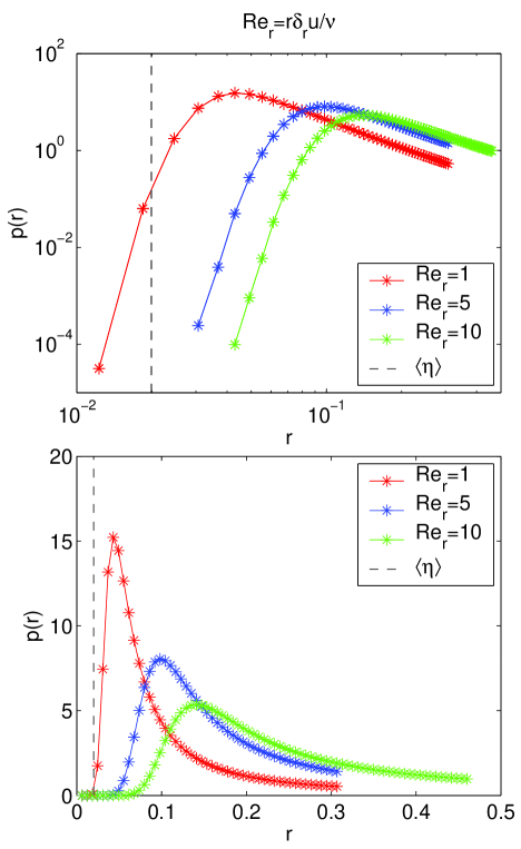
Figure 3: Logarithm of not normalized probability densitiy of the disspation scale $P(r=\eta_{c})\equiv Q(\frac{\eta_{c}}{\eta_{0}},Re)$ for $Re\approx 10^{3}$ and a few different values of parameter $a$. The PDFs were numerically evaluated by Schumacher (2007) using two different methods: 1. Algorithm based on the dissipation anomaly (eq. 2.1). (upper curve); 2  From the isolevels of dissipation rate ${\cal E}$. (lower curve). Broken lines denote Kolmogorov’s scale.

The theory presented in this paper is based on the dissipation scale definitions (2.1), (2.7),(2.8), derived from the dissipation anomaly. This algorithm was numerically compared by Schumacher (2007) with the one based on the isosurfaces of the scalar dissipation rate. The obtained PDFs $Q(\eta)$, though qualitatively similar, had quite substantial quantitative differences (see Fig. 3). Since the relations based on dissipation anomaly (2.1) have been derived directly from equations of motion, we believe they are much better justified.

Interesting and stimulating discussions with N. Peters, U. Frisch, A. Kerstein, J. Schumacher, E. Villermaux and K.R. Sreenivasan are gratefully aknowledged.

References

- (1) Batchelor, G.K. (1959) , J. Fluid Mech. 5, 113.
- (2) Bilger, R.W., 2004, Some aspects of scalar dissipation, Flow, Turbulence and Combustion 72, 93-114.
- (3) .Buch K.A. & Dahm W.J., J. Fluid Mech. 364, 1 (1998).
- (4) Celani, A, Cencini, M, Vergassola, M, Villermaux, E., & Vincenzi, D. 2005, Shear effects on passive scalar spectra, J.Fluid Mech. 523, 99-108.
- (5) Chertkov, M., Falkovich, G. & Kolokolov, I. 1998, Phys.Rev.Lett.80,2121. Dimotakis, P.E. 2005 Turbulent Mixing, Annu.Rev.Fluid Mech. 37, 329-356 (2005); Some issues on turbulence and turbulent mixing, CALCIT Report FM93-1. (March 1993).
- (6) Duchon, J. & Robert, R. (2000), Nonlinearity 13, 249
- (7) Eyink, G.L. 2003, Nonlinearity 16, 137 (2003).
- (8) Gamba, A. & Kolokolov, I. 1999, J.Stat.Phys. 94, 759.
- (9) Gotoh, T. & Nakano, T. 2003, J. Stat. Phys.113, 855.
- (10) Kushnir, D., Schumacher, & Brandt, A. 2006, Geometry of intensive dissipation events in turbulence., Phys. Rev. Lett. 97, 124502.
- (11) Landau, L.D. & Lifshitz, E.M. 1959, Fluid Mechanics, Pergamon Press, Oxford 1959.
- (12) Monin, A.S. & and Yaglom, A.M., Statistical Fluid Mechanics, vol. 2, MIT Press, Cambridge, MA .
- (13) Paladin, P. & Vulpiani, A. 1987, Phys.Rep. 156, 147 .
- (14) Peters, N., 2000, Turbulent Combustion, (Cambridge University Press, Cambridge, England, 2000).
- (15) Polyakov, A.M. 1995, Turbulence without pressure. Phys. Rev. E 52, 6183.
- (16) Schumacher, J. & Sreenivasan, K.R. (2003), Phys. Rev. Lett., 91, 174501.
- (17) Schumacher, J. 2007, Sub-Kolmogorov -Scale Fluctuations in Fluid Turbulence, Phys.Rev.Lett., (submitted).
- (18) Schumacher, J, Sreenivasan, K.R. & Yakhot, V. 2007, Asymptotic exponents from low -Reynolds -number flows, New. J. of Physics 9.
- (19) Sreenivasan, K.R. 2004, Possible effects of small-scale intermittency in turbulent reacting flows, Flow, Turbulence and Combustion 72, 115-131.
- (20) Tcheou, J.M., Brachet, M.E., Belin, F., Tabeling, P., & Wiliaime, H. 1999, Physica D, 129, 93-114.
- (21) Yakhot , V. & Sreenivasan, K.R. 2004, Physica A 343, 147-155.
- (22) Yakhot, V. & Sreenivasan, K.R. Anomalous scaling of structure functions and dynamic constraint on turbulence simulations, J. Stat. Phys.121 823, ( 2005).
- (23) Yakhot, V. 2006, Probability densities in strong turbulence, Physica D 215, 166, (2006).
- (24) Yakhot, V. 2003, Pressure-velocity correlations and anomalous exponents of structure functions in turbulence, J. Fluid Mech., 495, 135.