Automatic Active-Region Identification and Azimuth Disambiguation of the SOLIS/VSM Full-Disk Vector Magnetograms

Abstract

The Vector Spectromagnetograph (VSM) of the NSO’s Synoptic Optical Long-Term Investigations of the Sun (SOLIS) facility is now operational and obtains the first-ever vector magnetic field measurements of the entire visible solar hemisphere. To fully exploit the unprecedented SOLIS/VSM data, however, one must first address two critical problems: first, the study of solar active regions requires an automatic, physically intuitive, technique for active-region identification in the solar disk. Second, use of active-region vector magnetograms requires removal of the azimuthal $180^{o}$-ambiguity in the orientation of the transverse magnetic field component. Here we report on an effort to address both problems simultaneously and efficiently. To identify solar active regions we apply an algorithm designed to locate complex, flux-balanced, magnetic structures with a dominant E-W orientation on the disk. Each of the disk portions corresponding to active regions is thereafter extracted and subjected to the Nonpotential Magnetic Field Calculation (NPFC) method that provides a physically-intuitive solution of the $180^{o}$-ambiguity. Both algorithms have been integrated into the VSM data pipeline and operate in real time, without human intervention. We conclude that this combined approach can contribute meaningfully to our emerging capability for full-disk vector magnetography as pioneered by SOLIS today and will be carried out by ground-based and space-borne magnetographs in the future.

1. Introduction

SOLIS is a state-of-the art ground-based facility dedicated to the study of the Sun and its magnetic atmosphere for decades to come. It consists of three instruments - the vector spectromagnetograph (VSM), the Integrated Sunlight Spectrometer (ISS), and the Full-Disk Patrol (FDP). An overview on each instrument can be found in Keller, Harvey, & Giampapa (2003). The VSM, in particular, operates from Kitt Peak since May 2004. Among other daily measurements, the VSM performs complete Stokes polarimetry at the Fe I $630.2\;nm$ photospheric spectral line. An inversion of the Stokes images provides full-disk vector magnetograms of the solar photosphere (see Henney, Keller, & Harvey, 2006, for details). The VSM data are the first spectrographic full-disk vector magnetograms ever obtained. Partial-disk vector magnetography is performed by a handful of ground-based instruments and, recently, by the spectro-polarimeter of the Solar Optical Telescope (SOT) on board the Hinode satellite (Lites, Elmore, & Streander 2001). Hinode carries the first space-based vector magnetographs, while the first air-borne vector magnetograph was included in the Flare Genesis Experiment balloon payload (Rust, 1994). The first space-based full-disk vector magnetograms will be acquired by the Helioseismic and Magnetic Imager (HMI; Scherrer 2002) on board the imminent Solar Dynamics Observatory (SDO). From the above series of groundbreaking developments, one feels that solar vector magnetography is probably entering its golden era. Therefore, it is both essential and timely to address and efficiently solve the core problems associated with it in order to fully exploit the unprecedented existing and future vector magnetogram data.

Vector magnetic field measurements inferred by the Zeeman effect suffer from an intrinsic azimuthal ambiguity in the orientation of the transverse magnetic field component (Harvey, 1969). Indeed, the properties of the transverse Zeeman effect remain invariant under the transformation $\phi\rightarrow\phi+\pi$, where $\phi$ is the azimuth angle. The problem of the $180^{o}$-ambiguity has proved notoriously difficult to solve self-consistently, despite numerous attempts (for an overview, see Metcalf et al., 2006, and references therein). For full-disk magnetograms, an additional problem appears in case active regions should be studied. How are active regions to be extracted from the full-disk measurements? This task may appear trivial if performed manually, but it is quite daunting in case voluminous data are to be processed. Moreover, applications intimately related to active regions and their magnetic evolution such as, for example, magnetic helicity calculations or major flare forecasting, require a robust definition of active regions and their spatial extent.

In the following, we discuss our proposed solutions to both active region identification and azimuth disambiguation. Both techniques have been integrated into the VSM data pipeline and are operating in real time owing to the modest computational resources they require. Their operation is smooth and their solutions are robust, and this holds promise for automatic application to future full- or partial-disk vector magnetogram data.

2. VSM Data Processing

2.1. Automatic Identification of Solar Active Regions

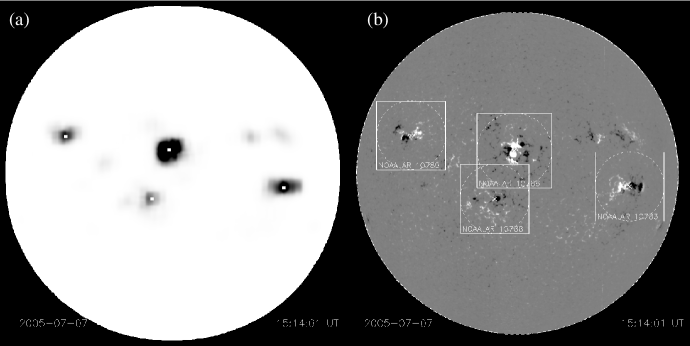
Figure 1.: Automatic active-region identification in a full-disk VSM magnetogram obtained on 2005 July 7, at around 15:14 UT. (a) Negative of the intensity image discussed in step 1. The centroid location for each qualifying intensity enhancement (see steps 2 and 3) is indicated by a white dot. Notice that some minor enhancements do not qualify for active-region association. (b) The final result of the identification process. Each active region is enclosed by a square prescribed to an outer circle from each centroid, as described in step (e). The corresponding NOAA numbers are also provided.

Our active-region identification method does not require vector magnetograms. It was conceived by B. J. LaBonte and was first applied by LaBonte, Georgoulis, & Rust (2007) to full-disk line-of-sight magnetograms of the Michelson-Doppler Imager (MDI - Scherrer et al., 1995) on board the Solar and Heliospheric Observatory (SoHO). The technique consists of five steps, namely:

1. Smooth the full-disk line-of-sight magnetic field $B_{\ell}$ using a smoothing window with linear size equal to one supergranular diameter (SGD), that is, $\sim 40\hbox{${}^{\prime\prime}$}$, or $\sim 30\;Mm$ on the solar surface. In the smoothed image, (i) test for bipolarity, enhancing magnetic polarity inversion lines, and (ii) calculate the gradient between the two polarities, emphasizing their E-W orientation. From this information (smoothed image, bipolarity, orientation) create an intensity image with enhancements corresponding to the active regions present on the disk (Figure 1a).

2. Coalign the intensity image with the actual magnetogram. Identify magnetic flux concentrations that coincide with the image’s enhancements and discard those with flux imbalance larger than a prescribed threshold.

3. For each qualifying intensity enhancement, determine an intensity-weighted centroid (barycenter).

4. Match the location of each centroid with NOAA’s Space Environment Center (SEC) archives to assign AR numbers to each centroid. For multiple numbers, choose the one with assigned location closest to the centroid.

5. Starting from each centroid, determine the spatial extent (area) of the respective active region.

Smoothing by 1 SGD provides a first clue of the existing active regions and their locations on the disk. The size of the smoothing window reflects the fact that supergranules are the fundamental convection cells responsible for the large-scale magnetic fields in the Sun and, therefore, for active-region formation (see, e.g., Leighton, Noyes, & Simon, 1962). The flux imbalance criterion points to the fact that active regions are mainly closed magnetic field structures. Nonetheless, the imbalance tolerance limit is an external variable and can be set at will. The dominant E-W orientation criterion helps avoid identifying accidental flux associations as active regions. The centroid calculation helps associate the identified flux concentrations with the standard NOAA active-region number database.

The remaining task is the determination of the spatial extent of each active region. This is accomplished in five steps, namely:

1. Draw two concentric circles around each centroid - an inner one with radius equal to 1 SGD and an outer one with radius equal to 6 SGD.

2. Define circles with increasing radii from 1 to 6 SGDs and find the average value of $|B_{\ell}|$ on each perimeter.

3. Find the median of the average $|B_{\ell}|$-values between 5 and 6 SGDs from the centroid. Use this median as a $1-\sigma$ threshold.

4. Check the perimeter averages of $|B_{\ell}|$ and stop at the circle where the average $|B_{\ell}|$ falls below $2\sigma$, i.e., becomes smaller than twice the above median.

5. Add 1 SGD to the radius of this circle and draw the square prescribed to this radius. This square will outline the edges of the identified active region (Figure 1b).

We underline that our size calculation technique, namely, defining an annulus with internal and external radius of 5 and 6 SGDs, respectively, to define the $1-\sigma$ threshold, precludes strong magnetic fields from being included in areas belonging to multiple active regions. Indeed, notice the overlapping between the areas of NOAA active regions (ARs) 10786 and 10788 in Figure 1b. This common area does not include strong magnetic fields. This stems from the fact that if the annulus cuts through strong magnetic flux accumulations, then the $1-\sigma$ threshold will be higher and the average $|B_{\ell}|$ value will drop below $2\sigma$ at shorter distances from the centroid, thereby imposing a smaller spatial extent for the examined active region. We have run numerous tests with full-disk magnetograms to verify that the technique performs as expected in the vast majority of cases.

2.2. Azimuth disambiguation

Our azimuth disambiguation method is the Nonpotential Magnetic Field Calculation (NPFC). The technique was introduced by Georgoulis (2005) and was slightly refined (NPFC2) as discussed in Metcalf et al. (2006). In this work, it was tested against several other techniques and was found to reproduce successfully the correct azimuth solution in highly nonpotential, noise-free, synthetic vector magnetograms. Moreover, it was among the fastest azimuth disambiguation techniques. In further comparisons, facilitated by a series of Azimuth Resolution Workshops, the NPFC2 method successfully reproduced the correct solution in nonpotential synthetic vector magnetograms where various levels of noise were embedded. Overall, the NPFC2 (hereafter NPFC) method demonstrated its speed and efficiency even in cases with extreme noise levels, that eventually led to its integration to the VSM software package.

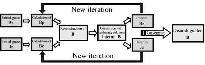
Figure 2.: A graphical description of the NPFC algorithm.

The physics behind the NPFC method is simple and starts by noticing that any magnetic field configuration $\mathbf{B}$ can be decomposed into a current-free (potential) component $\mathbf{B_{p}}$ and a current-carrying component $\mathbf{B_{c}}$, i.e.

$$\mathbf{B}=\mathbf{B_{p}}+\mathbf{B_{c}}\;\;.$$ (1)

If the magnetic structure is rooted in a lower boundary plane $S$ and extends in the half-space above it, then $\mathbf{B_{p}}$ and $\mathbf{B_{c}}$ can be calculated on $S$ provided that the vertical (normal to $S$) component $B_{z}$ of the magnetic field $\mathbf{B}$ and the vertical component $J_{z}$ of the electric current density $\mathbf{J}$ (where $\mathbf{J}$ is calculated by Ampere’s law), respectively, are known on $S$. For $\mathbf{B_{p}}$ there are multiple calculation methods including Green’s functions (Schmidt, 1964) and Fourier transforms (Alissandrakis, 1981). For $\mathbf{B_{c}}$, one utilizes the gauge conditions applying to $S$, and especially the fact that $\mathbf{B_{c}}$ has only an azimuthal component on $S$, i.e., $B_{c_{z}}|_{S}=0$. Assuming that $B_{c_{z}}$ does not vary significantly with height on $S$, i.e., $(\partial B_{c_{z}}/\partial z)|_{S}=0$, $\mathbf{B_{c}}$ can be calculated in Fourier space and then inverted into Cartesian space, i.e.,

$$\mathbf{B_{c}}=\mathcal{F}^{-1}[{{ik_{y}}\over{k^{2}}}\mathcal{F}(j_{z})]\mathbf{\hat{x}}+\mathcal{F}^{-1}[{{-ik_{x}}\over{k^{2}}}\mathcal{F}(j_{z})]\mathbf{\hat{y}}\;\;.$$ (2)

In Equation (2) we have $k^{2}=k_{x}^{2}+k_{y}^{2}$ for the harmonic $(k_{x},k_{y})$ and $j_{z}=(4\pi/c)J_{z}$, while $\mathcal{F}(r)$, $\mathcal{F}^{-1}(r)$ are the direct and inverse Fourier transforms of $r$, respectively, at $(k_{x},k_{y})$. Notice that the only assumption of the NPFC method is $(\partial B_{c_{z}}/\partial z)|_{S}=0$. This assumption is quite reasonable because $B_{c_{z}}|_{S}=0$ and, for small length elements, one might expect that $B_{c_{z}}\simeq 0$ slightly above $S$, unless the magnetic field lines undergo dramatic changes of orientation within the elementary height. Assuming that $S$ is the plane of the magnetic field measurements, an unambiguous magnetic field $\mathbf{B}$ can be reconstructed on this plane from $\mathbf{B_{p}}$ and $\mathbf{B_{c}}$. The problem, of course, is that both $B_{z}$ and $J_{z}$, required to calculate $\mathbf{B_{p}}$ and $\mathbf{B_{c}}$, respectively, are subject to the $180^{o}$-ambiguity and are not known a priori. This is where the numerical part of the NPFC method begins.

Figure 2 provides a graphical representation of the numerical process. Initial-guess distributions of $B_{z}$ and $J_{z}$ are used to calculate the initial-guess $\mathbf{B_{p}}$ and $\mathbf{B_{c}}$, respectively. The total field $\mathbf{B}$ is then reconstructed through Equation (1). The reconstructed field is compared to the two equally possible ambiguity solutions and is set equal to the solution that is closer to it, for each location of the measurements’ plane. This interim $\mathbf{B}$-configuration gives rise to new $B_{z}$- and $J_{z}$-solutions. From them, new $\mathbf{B_{p}}$- and $\mathbf{B_{c}}$-configurations are produced, and the algorithm proceeds to a new iteration. Convergence is judged by the number of strong-field vectors whose orientation changes from one iteration to the next. When no vectors (or a small number of vectors) are flipped for 10 consecutive iterations, the process stops and the latest reconstructed $\mathbf{B}$-configuration is the suggested disambiguation solution.

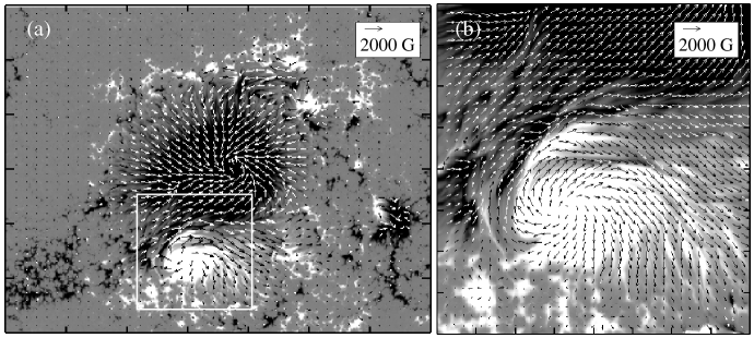
Figure 3.: Example of the NPFC disambiguation solution. Shown are the heliographic magnetic field components on the image plane. (a) The solution on part of a Hinode/SOT spectro-polarimeter vector magnetogram depicting NOAA AR 10930, obtained on 2006 December 11 between 13:53 UT and 15:15 UT. The data features a sunspot complex separated by a strongly sheared magnetic polarity inversion line, enclosed by the white square. Tick mark separation is $20\hbox{${}^{\prime\prime}$}$. (b) The disambiguation solution for the enclosed area. Tick mark separation is $5\hbox{${}^{\prime\prime}$}$. In both images, the vertical magnetic field saturates at $\pm 1000\;G$. Data courtesy of B. W. Lites.

The entire calculation requires minimal computing resources and is completed in a matter of minutes, even at an ordinary desktop workstation. Remarkably, the speed of the convergence does not depend on the complexity of the studied magnetogram but, rather, on its quality and linear size. In other words, the quality of the solution depends strongly on the quality of the measurements. To demonstrate this, we show in Figure 3 a disambiguated vector magnetogram from Hinode’s SOT spectro-polarimeter that was inverted and kindly provided to us by B. W. Lites. These data are of exceptionally high seeing-free quality and nearly unsurpassed spatial resolution ($\sim 0.16\hbox{${}^{\prime\prime}$}$ per pixel). The depicted active region (NOAA AR 10930) shows a significant degree of complexity, especially along a strongly sheared magnetic polarity inversion line. The magnetogram’s field of view had a very large linear size, namely, $1904\times 1024$ pixels. Yet the NPFC method required only $\sim 20\;min$ and $34$ iterations to converge. The respective computing time for typical linear dimensions of, say, $512\times 512$ pixels, would not exceed $2\;min$.

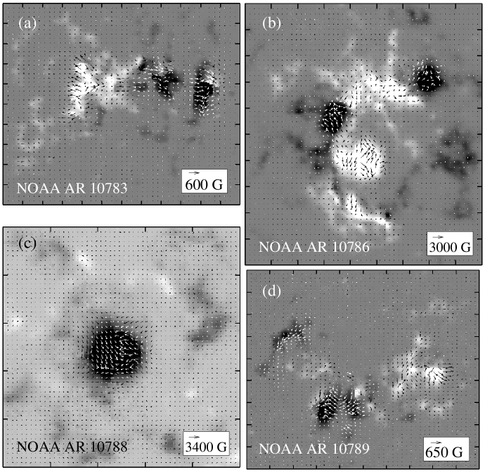
Figure 4.: The NPFC disambiguation solutions for the four active regions identified in the VSM magnetogram of Figure 1. Shown are the heliographic magnetic field components on the image plane. The solutions are given for a part of the area assigned to each region, namely, the part containing the majority of the active-region magnetic flux. Tick mark separation in all images is $20\hbox{${}^{\prime\prime}$}$. The vertical magnetic field in all images saturates at $\pm 1000\;G$.

Figure 4 provides the NPFC disambiguation solutions for the active regions identified in the VSM magnetogram of Figure 1. Inspecting Figure 4, one might notice some inconsistencies in the orientation of the horizontal magnetic field. These imperfections should be mostly attributed to problems in the inference of the VSM azimuth angle. Indeed, the VSM measurements at the time of the observation (07/07/05) were still quite preliminary, with now-known issues not addressed in the data. The reason why we chose to show these data, nevertheless, is the high degree of activity in the solar atmosphere at the time of the observation. Vector magnetograms obtained thereafter showed much less activity and fewer, simpler, active regions, although the inference of the azimuth angle was drastically improved. In the near future, when solar activity will start stepping up toward the next maximum, the VSM will be fully equipped with sufficient hardware and software to reliably acquire and process massive amounts of data.

3. Conclusions / Current status of the VSM vector magnetogram data

Although VSM full-disk vector magnetograms at the Fe I $630.2\;nm$ photospheric line are obtained since August 2003, these data have not yet been released to the solar and space physics communities. This is due to work currently underway on the last remaining issues that, however, must be addressed prior to releasing any digital data. This being said, we are confident that the data will be available for unrestricted use very soon.

Complete descriptions of VSM and its data archive can be found at
ttp://solis.nso.edu/solis_data.tml. Among other information, this web page includes quick-look visualizations of both the latest VSM vector magnetograms and the regularly updated list of the VSM vector magnetogram data archive. Featuring a user-friendly interface, one may view all the magnetic field components for each identified active region, together with the zenith and azimuth angles of the disambiguated magnetic field vector. Upon the release of the VSM data, full Milne-Eddington inversion products will be available nearly 24 hours after the quick-look data acquisition (Henney, Keller, & Harvey, 2006).

As for the active-region identification and azimuth disambiguation techniques, this article demonstrates that they are general enough to be applied to both existing and future vector magnetograms, either in conjunction or independently. Partial-disk magnetograms (e.g., from Hinode) might be disambiguated using the NPFC method, while future SDO/HMI full-disk magnetograms might undergo a process similar to that described in §2 for the SOLIS/VSM data.

Acknowledgments.

SOLIS/VSM data used here are produced cooperatively by NSF/NSO and NASA/LWS. The National Solar Observatory is operated by AURA, Inc. under a cooperative agreement with the National Science Foundation. We are grateful to B. W. Lites for providing us with the inverted spectro-polarimeter data from Hinode/SOT. Hinode is a Japanese mission developed and launched by ISAS/JAXA, with NAOJ as domestic partner and NASA and STFC (UK) as international partners. It is operated by these agencies in co-operation with ESA and NSC (Norway). The azimuth disambiguation and active-region identification studies have received partial support by the NASA LWS TR&T Grant NNG05-GM47G. N.-E. R.’s work is supported by the NSO and NASA Grant NNH05AA12I.

References

- (1) Alissandrakis, C. E., 1981, A&A, 100, 197
- (2) Georgoulis, M. K., 2005, ApJ, 629, L69
- (3) Harvey, J. W., 1969, Ph.D. Thesis, Univ. Colorado
- (4) Henney, C. J., Keller, C. U., & Harvey, J. W., 2006, ASP Conf. Series, 358, 92
- (5) Keller, C. U., Harvey, J. W., & Giampapa, M. S., 2003, Proc. SPIE, 4853, 114
- (6) LaBonte, B. J., Georgoulis, M. K., & Rust, D. M., 2007, ApJ, submitted
- (7) Leighton, R. B., Noyes, R. W., & Simon, G. W., 1962, ApJ, 135, 474
- (8) Lites, B. W., Elmore, D. F., & Streander, K. D., 2001, in Advanced Solar Polarimetry - Theory, Observation, and Instrumentation, ed. M. Sigwarth (San Francisco: ASP), PASP, 236, 33
- (9) Metcalf, Th. R., Leka, K. D., Barnes, G., Lites, B. W., Georgoulis, M. K., Pevtsov, A. A., Balasubramaniam, K. S., Gary, G. A., Jing, J., Li, J., Liu, Y., Wang, H. N., Abramenko, V., Yurchyshyn, V., & Moon, Y.-J., 2006, Solar Phys., 237, 267
- (10) Rust, D. M., 1994, Adv. Space Res., 14(2), 89
- (11) Scherrer, P. H., 2002, AGU Fall Meeting, abstract #SH52A-0494
- (12) Scherrer, P. ., Bogart, R. S., Bush, R. I., Hoeksema, J. T., Kosovichev, A. G., Schou, J., Rosenberg, W., Springer, L., Tarbell, T. D., Title, A., Wolfson, C. J., Zayer, I., & the MDI Engineering Team, 1995, Solar Phys., 162, 129
- (13) Schmidt, H. U., 1964, in The Physics of Solar Flares, ed. W. N. Hess (NASA SP-50; Washington DC; NASA), 107