The order-disorder transition in colloidal suspensions under shear flow

Abstract

We study the order-disorder transition in colloidal suspensions under shear flow by performing Brownian dynamics simulations. We characterize the transition in terms of a statistical property of time-dependent maximum value of the structure factor. We find that its power spectrum exhibits the power-law behaviour only in the ordered phase. The power-law exponent is approximately -2 at frequencies greater than the magnitude of the shear rate, while the power spectrum exhibits the $1/f$-type fluctuations in the lower frequency regime.

1 Introduction

Order-disorder transitions such as solid-liquid transitions and ferromagnetic transitions are distinctive phenomena in equilibrium systems. The understanding of the transitions has been a cornerstone for developments in equilibrium statistical mechanics. Here, the notion of “order” is not restricted to equilibrium systems. For example, one can modify a system exhibiting the order-disorder transition under equilibrium conditions so that it can be observed even under non-equilibrium conditions. Since non-equilibrium statistical mechanics has not been established as yet, there is no systematic understanding of this type of transition from the viewpoint of statistical mechanics. Therefore, it is important to study a typical example related to this question.

As a simple and realistic example, we consider a system consisting of colloidal particles suspended in a liquid. It is known that this system exhibits an order-disorder transition under equilibrium conditions. In particular, the so-called “colloidal crystal” is observed in the ordered phase. This system may be regarded as an ideal model system because one can observe such a crystalline structure by using a microscope and also because one can control the system as desired.

Recently, a couple of experiments have been reported on colloidal suspensions under shear flow [1, 2]. Holmqvist et al. obtained the phase diagram for colloidal suspensions under stationary Couette flow. They observed Bragg reflections of laser light and measured the Bragg peak intensity of the first Debye-Scherrer ring. From the time dependence of the total Bragg peak intensity, they determined the crystal growth rate and induction time. The phase boundary in their phase diagram is determined by extrapolating the growth rate and induction time are extrapolated to zero.

Furthermore, there are several reports on numerical experiments of colloidal suspensions under shear flow. Butler and Harrowell performed Brownian dynamics simulations of colloidal particles under shear flow [3, 4]. They obtained a phase diagram of temperature versus shear rate. The phase boundary of their phase diagram was determined from the long-time average of the intensity of the Bragg peak with the wavevector aligned in the shear gradient direction. The ‘order’ in their paper was assumed to appear when the intensity exceeded half of the intensity value for scattering from a body-centred cubic crystal aligned in the direction of the velocity gradient.

These results suggest the existence of the order-disorder transition. Here, let us recall that crystal is defined as the state with a translational symmetry breaking. Thus, if we attempt to determine the ‘crystal’ phase, we should investigate the structure factor $S(k)$ for systems under shear flow. However, from a simple consideration, we find that there is no crystal phase in the rigorous sense, even if the existence of an ordered state is suggested by several measurements. Now, the objective of this study is to find a useful and thorough characterization of the ordered state for systems under shear flow. We attempt this characterization by performing Brownian dynamics simulations of the colloidal suspensions under shear flow.

This paper is organized as follows. In section 2, the model that is investigated is introduced. Further, before discussing non-equilibrium cases in section 3 as preliminaries, we review the order-disorder (crystal-fluid) transition under equilibrium conditions and confirm the conventional criteria for the crystallization. Section 3 comprises the main part of this paper. We characterize the ordered phase in terms of the time-dependent quantity $s_{\mathrm{m}}(t)$, which is defined as the first maximum of the structure factor $\hat{s}(k,t)$ for configuration of the particles at time $t$. We find that $\tilde{S}_{\mathrm{m}}(\omega)$, which is the power spectrum of $s_{\mathrm{m}}(t)$, exhibits a clear transition when the temperature is changed. Concretely, in the ordered phase, the power spectrum exhibits the power-law behaviour, and there are two different power-law exponent regimes divided by the crossover frequency that is determined by the shear rate $\dot{\gamma}$: $\tilde{S}_{\mathrm{m}}(\omega)\simeq\omega^{-2}$ in the high frequency regime ($\omega\gtrsim 2\pi\dot{\gamma}$) and $1/f$-type fluctuations in the low frequency regime ($\omega\lesssim 2\pi\dot{\gamma}$). Meanwhile, $\tilde{S}_{\mathrm{m}}(\omega)$ in the disordered phase is similar to the white noise spectrum. Future problems are presented in the final section.

2 Preliminaries

We consider a system consisting of $N$ colloidal particles suspended in a fluid where the stationary planar shear flow is realized. The system is confined to a cubic cell with a length $L$. The $x$-axis and $z$-axis are chosen to be the directions of the shear velocity and velocity gradient, respectively. We impose Lees-Edwards periodic boundary conditions [5, 6] to avoid peculiarities near the boundaries of the cell.

We assume that Langevin dynamics can describe the motion of the colloidal particles. Concretely, the force exerted from the fluid is represented by the Stokes force and Gaussian noise. In other words, we neglect the so-called hydrodynamic effects. Then, the particle positions $\mbox{\boldmath{$r$}}_{i}(t)=(x_{i}(t),y_{i}(t),z_{i}(t))$, where $1\leq i\leq N$, obey the Langevin equations

$$\eta\frac{\mathrm{d}\mbox{\boldmath{$r$}}_{i}}{\mathrm{d}t}=-\sum_{j\neq i}\nabla U(|\mbox{\boldmath{$r$}}_{i}-\mbox{\boldmath{$r$}}_{j}|)+\dot{\gamma}z_{i}(t)\mbox{\boldmath{$e$}}_{x}+\mbox{\boldmath{$\xi$}}_{i}(t),$$ (1)

where $\eta$ is a friction coefficient; $\dot{\gamma}$, the shear rate; and $\mbox{\boldmath{$e$}}_{x}$, the unit vector that is parallel to the $x$-axis. The variable $\mbox{\boldmath{$\xi$}}_{i}(t)=(\xi_{i}^{x}(t),\xi_{i}^{y}(t),\xi_{i}^{z}(t))$ represents the Gaussian noise that satisfies

$$\left<\xi_{i}^{\alpha}(t)\xi_{j}^{\beta}(t^{\prime})\right>=2\eta k_{\mathrm{B}}T\delta_{ij}\delta^{\alpha\beta}\delta(t-t^{\prime}).$$ (2)

Here, $k_{\mathrm{B}}$ is the Boltzmann constant and $T$ is the temperature. The superscripts $\alpha$ and $\beta$ represent the Cartesian components. Each pair of particles interacts via a screened Yukawa potential

$$U(r)=\left\{\begin{array}[]{ll}\displaystyle U_{0}\sigma\left(\frac{\exp(-\kappa(r-\sigma))}{r}-\frac{\exp(-\kappa(r_{\mathrm{c}}-\sigma))}{r_{\mathrm{c}}}\right),&\mbox{if $r\leq r_{\mathrm{c}}$},\\ 0,&\mbox{otherwise}.\end{array}\right.$$ (5)

Here, $r$ is the distance between the particles; $r_{\mathrm{c}}$, the cutoff length that simplifies the calculation in numerical simulations; and $\kappa$, a Debye screening parameter.

In this study, all the quantities are converted to dimensionless forms by setting $\sigma=U_{0}=\eta/k_{\mathrm{B}}T=k_{\mathrm{B}}=1$. We estimate the correspondence between these parameters and those of real experimental systems to be $\sigma\sim 10^{2}$ nm, $U_{0}\sim 10k_{\mathrm{B}}T$ and $k_{\mathrm{B}}T/\eta=10^{-11}{\mathrm{m}}^{2}{\mathrm{s}}^{-1}$. In our simulation, we assume that $\kappa\sigma=5.8$, $L/\sigma=10$, $r_{\mathrm{c}}=2.5$ and $N\sigma^{3}/L^{3}=1$. In other words, the Debye screening length $\kappa^{-1}$ corresponds to $17$ nm. The typical values of the parameters used in our simulations are $T\sim 0.1$ and $\dot{\gamma}=0.001$, and this situation corresponds to experimental systems wherein the temperature is 300 K and the shear rate is 1 $\mathrm{s}^{-1}$. The systems that have the values are available by laboratory experiments.

In our simulations, we discretized (1) with the time step $\Delta t=0.0025$. Note that in the arguments below, $\left<\cdots\right>$ represents the statistical average in the steady states. In the calculation we performed, we estimated $\left<A\right>$ to be $\int_{t_{0}}^{t_{0}+\tau}dtA(t)/\tau$, where $t_{0}$ and $\tau$ were chosen as that larger than $10^{3}$, because we had confirmed that the relaxation time is approximately $10^{2}$.

Before considering the behaviour of colloidal suspensions under shear flow, we review the transition observed in the system under the equilibrium condition ($\dot{\gamma}=0$). It is expected that the crystalline arrangement of colloidal particles is observed in the ordered phase of this system, while they acquire a random configuration in the disordered phase. In order to detect the order-disorder transition, one relies on the definition of a crystal according to which the statistical weight for configurations of colloidal particles breaks translational and rotational symmetries. The translational symmetry breaking can be quantified by $S(k)$, which is defined as

$$S(k)=\left<\frac{1}{4\pi}\int_{0}^{2\pi}\mathrm{d}\phi\int_{0}^{\pi}\mathrm{d}\theta\,\sin\theta\,\frac{1}{N}|\tilde{\rho}(\mbox{\boldmath{$k$}})|^{2}\right>.$$ (6)

Here, the angles $\theta$ and $\phi$ are defined as $\mbox{\boldmath{$k$}}=(k\cos\phi\sin\theta,k\sin\phi\sin\theta,k\cos\theta)$ with $k=|\mbox{\boldmath{$k$}}|$, and $\tilde{\rho}(\mbox{\boldmath{$k$}})$ is the Fourier transform of the number density $\rho(\mbox{\boldmath{$r$}})$:

$$\tilde{\rho}(\mbox{\boldmath{$k$}})=\int_{-\infty}^{\infty}\!\mathrm{d}^{3}\mbox{\boldmath{$r$}}\,\rho(\mbox{\boldmath{$r$}})\exp(-i\mbox{\boldmath{$k$}}\cdot\mbox{\boldmath{$r$}})$$ (7)

with

$$\rho(\mbox{\boldmath{$r$}})=\frac{1}{N}\sum_{i=1}^{N}\delta(\mbox{\boldmath{$r$}}-\mbox{\boldmath{$r$}}_{i}).$$ (8)

When $S(k)$ has a component that is expressed by Dirac’s delta function, the system is assumed to exhibit the translational symmetry breaking. Note that $S(k)$ can be measured experimentally because it is related to the Bragg peak intensity of the laser light scattering.

In our simulations, instead of $S(k)$, we use $S_{L}(k)$ defined by

$$S_{L}(k)=1+4\pi\rho\int_{0}^{L/2}\mathrm{d}r\,(\left<g(r;\{\mbox{\boldmath{$r$}}_{i}\})\right>-1)\frac{\sin(kr)}{kr}\frac{\sin(2\pi r/L)}{2\pi r/L},$$ (9)

where $\hat{g}(r;\{\mbox{\boldmath{$r$}}_{i}\})$ represents the radial distribution function for a given configuration $\{\mbox{\boldmath{$r$}}_{i}\}$, that is,

$$\hat{g}(r;\{\mbox{\boldmath{$r$}}_{i}\})=\frac{1}{4\pi\rho r^{2}}\frac{\mathrm{d}n(r)}{\mathrm{d}r}.$$ (10)

Here, $\mathrm{d}n(r)$ is the average number of particles at distances between $r$ and $r+\mathrm{d}r$ from any particle, and its average is taken over all the particles. Note that $\left<\hat{g}(r;\{\mbox{\boldmath{$r$}}_{i}\})\right>$ is equal to the standard radial distribution function $g(r)$. It should be noted that $g(r)$ is defined in the range where $r\leq L/2$, owing to the periodic boundary conditions. The term $\sin(2\pi r/L)/(2\pi r/L)$ appended in the integrand is the window function to reduce the termination effects resulting from the finite upper limit [7, 8]. Note that $S_{L}(k)$, as defined above, approaches $S(k)$ in the thermodynamic limit $L\rightarrow\infty$.

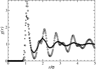
Figure 1: Plot of $g(r)$ against $r/\sigma$. $T=$ 0.12 ($\opencircle$: open circles) and 0.18 ($\ast$: stars) under equilibrium conditions.

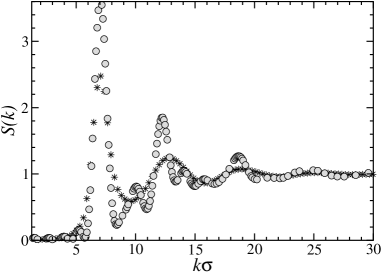
Figure 2: Plot of $S_{L}(k)$ against $k\sigma$. $T=$ 0.12 ($\opencircle$: open circles) and 0.18 ($\ast$: stars) under equilibrium conditions..

As observed in figure 2, we cannot observe infinitely sharp peaks owing to finite size effects. However, it is known that there are empirical criteria for detecting the transition; one of these criteria is Hansen-Verlet’s rule [9, 10]. According to this rule, a fluid freezes when the first maximum value of the static structure factor $S_{\mathrm{m}}$ exceeds 2.85. This criterion has been tested and validated for various systems [9, 11]. Indeed, in our system, we find that $S_{\mathrm{m}}$ exhibits a discontinuous jump at the transition temperature $T_{\mathrm{c}}$ whose value is estimated between 0.16 and 0.165, as shown in figure 4. Further, when the temperature $T$ is lower than the transition temperature $T_{\mathrm{c}}$, $S_{\mathrm{m}}$ exceeds 2.85, while $S_{\mathrm{m}}$ is less than 2.85 in the higher temperature regime. Thus, we conclude that the order-disorder transition is observed.

As another order parameter for indicating the phase transition, we consider the bond-orientational order parameter $Q_{\mathrm{6}}$ [12, 13], which is determined by the set of bond vectors $\{\hat{\mbox{\boldmath{$r$}}}_{i}\}$ as follows:

$$Q_{\mathrm{6}}=\left<\left(\frac{4\pi}{13}\sum^{6}_{l=-6}|\bar{Q}_{\mathrm{6}}^{l}|^{2}\right)^{1/2}\right>,$$ (11)

with

$$\bar{Q}_{6}^{l}=\frac{1}{N_{\mathrm{b}}}\sum^{N_{\mathrm{b}}}_{i=1}Y_{6}^{l}(\theta(\hat{\mbox{\boldmath{$r$}}}_{i}),\phi(\hat{\mbox{\boldmath{$r$}}}_{i})).$$ (12)

Here, each bond vector $\hat{\mbox{\boldmath{$r$}}_{i}}$ corresponds to the relative vector between the neighbouring particles; $N_{\mathrm{b}}$ is the number of bond vectors; $Y_{\mathrm{6}}^{l}$, the spherical harmonics function of degree six; and $\theta(\hat{\mbox{\boldmath{$r$}}}_{i})$ and $\phi(\hat{\mbox{\boldmath{$r$}}}_{i})$, the polar and azimuthal angles of $\hat{\mbox{\boldmath{$r$}}}_{i}$, respectively. Here, we have defined the neighbouring particles for a given particle as those within the sphere of radius $r_{\mathrm{c}}$ around the given particle, where $r_{\mathrm{c}}$ is chosen as the first minimum of $g(r)$. The quantity $Q_{\mathrm{6}}$ represents the degree of breakage of the continuous rotational symmetries, particularly, the 6-fold rotational symmetry of the configuration of the particles. Its value is 0.57452 for a face-centred cubic (fcc) crystal, 0.51069 for a body-centred cubic (bcc) crystal and 0 for liquids. We show the temperature dependence of $Q_{\mathrm{6}}$ in figure 4. It is observed that $Q_{\mathrm{6}}$ decreases between $T=0.16$ and $T=0.165$ in a discontinuous manner. This result is consistent with that indicated by Hansen-Verlet’s rule.

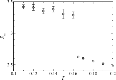
Figure 3: $S_{\mathrm{m}}$ as a function of $T$ under the equilibrium condition $\dot{\gamma}=0$. The average values with error bars are displayed using 10 samples for each temperature.

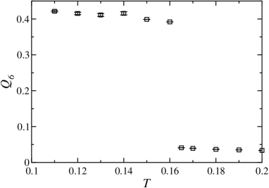
Figure 4: $Q_{\mathrm{6}}$ as a function of $T$ under the equilibrium condition $\dot{\gamma}=0$. The average values with error bars are displayed using 10 samples for each temperature.

3 Question and Result

Even for colloidal suspensions under shear flow, we can measure $S(k)$ and $Q_{\mathrm{6}}$ in a manner identical to that of the equilibrium cases. The results with $\dot{\gamma}=0.001$ are displayed in figures 6 and 6. These graphs are similar to those for the equilibrium system. In the temperature regime lower than $T=0.16$, $S_{\mathrm{m}}$ exceeds 2.85, while it dips from 2.85 in the regime higher than $T=0.17$. Apparently, this result indicates the existence of an order-disorder transition in this situation. Similarly, $Q_{\mathrm{6}}$ shows a clear difference between the low temperature regime and the high temperature regime, as shown in figure 6.

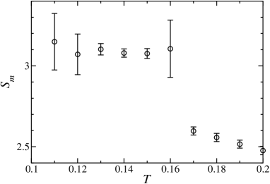
Figure 5: $S_{\mathrm{m}}$ as a function of $T$ at $\dot{\gamma}=0.001$. The average values with the error bars are displayed using 10 samples for each temperature.

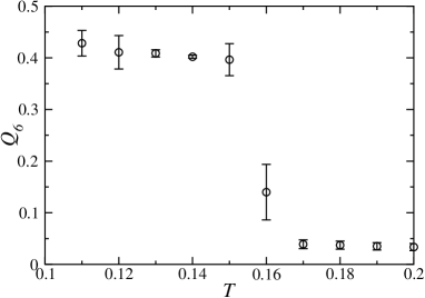
Figure 6: $Q_{\mathrm{6}}$ as a function of $T$ at $\dot{\gamma}=0.001$. The average values with the error bars are displayed using 10 samples for each temperature.

We recall that a crystal is defined as the state that breaks the translational symmetry of the statistical weight for the configurations of the particles. In order to simplify the above argument, we first consider the case $T=0$ where particles move coherently and form two-dimensional crystals in $(x,y)$ planes for a fixed $z$. In this state, the translational symmetries in the $x$ and $y$ directions are broken for a given $z$. However, the spatial period in the $z$ direction is time dependent. Thus, by considering the ensembles generated by the time evolution, we expect that the translational symmetry in the $z$ direction recovers. Next, we consider the finite temperature cases. A translational symmetry is expected to exist in the $z$ direction, and according to Mermin-Wagner’s theorem, which states that there is no translational symmetry breaking in two-dimensional systems, we do not expect the symmetry breaking to occur in the $(x,y)$ planes. Thus, we conclude that there is no crystal in colloidal suspensions under shear flow.

Although the structure factor does not involve Dirac’s delta peak even in the thermodynamics limit, figures 6 and 6 suggest the existence of a discontinuous transition. Therefore, the nature of this transition should be different from that in equilibrium systems. In order to further clarify the above difference, we attempt to study this transition from another viewpoint.

In particular, we consider the dynamical features of non-equilibrium systems possess. First, let us observe the variation of the structure factor with time. As an example, we define the time-dependent structure factor $\hat{s}(k,t)$ that is determined for each particle configuration $\{\mbox{\boldmath{$r$}}_{i}(t)\}$ at time $t$:

$$\hat{s}(k,t)=1+4\pi\rho\int_{0}^{R}\mathrm{d}r\,(g(r;\{\mbox{\boldmath{$r$}}_{i}(t)\})-1)\frac{\sin(kr)}{kr}\frac{\sin(2\pi r/L)}{2\pi r/L}.$$ (13)

Note that $S_{L}(k)$ defined in (9) is equal to $\left<\hat{s}(k,t)\right>$. In figure 7, the results for two different cases $T=0.14$ and $0.18$ are displayed by fixing the shear rate to be $\dot{\gamma}=0.001$. From this figure, it is observed that the maximum intensity of $\hat{s}(k,t)$ at $T=0.14$ varies with time more significantly than that at $T=0.18$. Since there appears to be a qualitative difference, we focus on the time dependence of the first maximum of $\hat{s}(k,t)$ with respect to $k$, which is denoted by $s_{\mathrm{m}}(t)$.

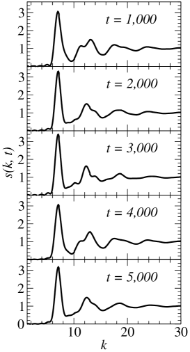
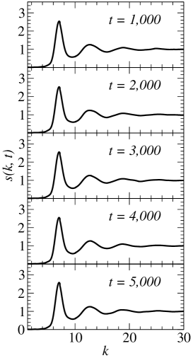
Figure 7: Time evolution of the structure factor for $T=0.14$ (left) and $T=0.18$ (right).

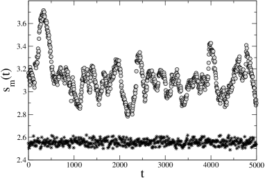
Figure 8: $s_{\mathrm{m}}(t)$ for $T=0.14$ ($\opencircle$: open circles) and $T=0.18$ ($\ast$: stars).

In figure 8, typical data of $s_{\mathrm{m}}(t)$ are displayed. It is clearly observed that $s_{\mathrm{m}}(t)$ exhibits a considerably larger fluctuation in the low temperature case ($T=0.14$) as compared to that in the high temperature case ($T=0.18$). In order to characterize the difference between the two cases quantitatively, we consider the spectra of the fluctuations, which are defined by

$$\tilde{S}_{m}(\omega)=\left<\left|\int_{-\infty}^{\infty}\mathrm{d}t\,s_{\mathrm{m}}(t)\exp(-i\omega t)\right|^{2}\right>.$$ (14)

The shapes of the power spectra shown in figure 9 indicate a distinct transition at a certain temperature $T_{\mathrm{c}}$. Indeed, for the temperatures $T=0.14$ and 0.16, the power-law behaviour $\tilde{S}_{m}(\omega)\simeq\omega^{-2}$ is observed in the frequency regime $\omega\geq 2\pi\dot{\gamma}$. Moreover, focusing on the behaviour in the low frequency regime $\omega\leq 2\pi\dot{\gamma}$, we observe the $1/f$-type fluctuation. Meanwhile, the spectrum becomes flat at the temperature $T=0.18$. Therefore, for example, by plotting $\tilde{S}_{m}(2\pi\dot{\gamma})$ against $T$, we can observe a discontinuous transition at $T=T_{\mathrm{c}}$, as shown in figure 10.

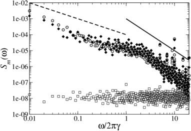
Figure 9: Spectra $\tilde{S}_{\mathrm{m}}(\omega)$ as a function of $\Omega=\omega/2\pi\dot{\gamma}$. $T=0.14$ (closed diamonds), 0.16 (open circles) and 0.18 (stars). The solid line represents the $\omega^{-2}$ slope, and the dashed line denotes the $\omega^{-1}$ slope.

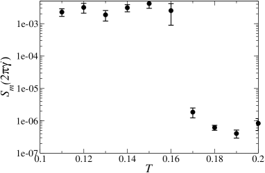
Figure 10: $\tilde{S}_{m}(2\pi\dot{\gamma})$ as a function of $T$. The average values with error bars are determined by using 10 samples for each temperature.

4 Concluding Remarks

The results in this paper motivate us to study the system in more detail. Before concluding the paper, we address two important future problems. First, the mechanism of the power-law behaviours of $\tilde{S}_{m}(\omega)$ should be elucidated on the basis of “defects” in the ordered phase. After defining the defects in a suitable manner, we may quantitatively characterize the destruction of the crystal-like structure and its subsequent restoration with time. It is natural to conjecture that the power-law behaviour $\tilde{S}_{m}(\omega)\simeq\omega^{-2}$ might be related to the generation and annihilation of defects in the ordered phase under shear flow. Therefore, by focusing on the elementary processes of defect dynamics, we may understand this power-law behaviour. Furthermore, the power-law behaviour $\tilde{S}_{m}(\omega)\simeq\omega^{-1}$ observed in the low frequency regime suggests the existence of a more complex mechanism. As one possibility, a cooperative phenomenon involving the ‘defects’ may occur. In order to explore this possibility, we should investigate the spatial correlation of the dynamical events of the defects.

The second problem is related to the thermodynamic aspects of the order-disorder transition in colloidal dispersions under shear flow. From the analogy of the order-disorder transition in equilibrium systems, we conjecture the existence of a latent heat associated with the order-disorder transitions in non-equilibrium systems. However, the heat is apparently generated because the system is in a non-equilibrium steady state. With regard to this problem, Oono and Paniconi proposed a remarkable concept in which the excess heat plays a prominent role in a thermodynamic framework for non-equilibrium steady states [14]. Indeed, by employing this quantity, the second law of thermodynamics has been extended to transitions between non-equilibrium steady states within the Langevin description [15]. Thus, we can consider the latent (excess) heat even for colloidal suspensions under shear flow.

In summary, we have characterized the order-disorder transition of colloidal suspensions under shear flow by employing dynamical features of the structure factor because there exists no ‘crystal’ under the shear flow. Defining a new order parameter $\tilde{S}(\omega)$, we have detected the transition by measuring the temperature dependence of $\tilde{S}(2\pi\dot{\gamma})$, as shown in figure 10. We also have found that the discontinuous transition accompanies the $1/f$-type fluctuations in the low frequency regime. By a more detailed study of the above-mentioned problems, we hope to gain a thorough understanding of the nature of non-equilibrium phase transitions.

References

References

- [1] Tsuchida A, Takyo E, Taguchi K and Okubo T 2004 Colloid Polym. Sci. 282 1105
- [2] Holmqvist P, Lettinga M P, Buitenhuis J and Dhont J K G 2005 Langmuir 21 10976
- [3] Butler S and Harrowel P 1995 J. Chem. Phys.103 4653
- [4] Butler S and Harrowel P 1995 Phys. Rev. A 52 6424
- [5] Lees A W and Edwards S F 1972 J. Phys. C: Solid State Phys.5 1921
- [6] Evans D J and Morriss G P 1990 Statistical Mechanics of Nonequilibrium Liquids (Academic Press, New York)
- [7] Lorch E A 1969 J. Phys. C: Solid State Phys.2 229
- [8] Guitiérrez G and Rogan J 2004 Phys. Rev. E 69 031201
- [9] Hansen J-P and Verlet L 1969 Phys. Rev.184 151
- [10] Löwen H and Hoffman G P 2001 J. Phys.: Condens. Matter13 9197
- [11] Blaak R, Auer S, Frenkel D and Löwen H 2004 Phys. Rev. Lett.93 068303
- [12] Steinhardt P J, Nelson D R and Ronchetti M 1983 Phys. Rev. B 28 784
- [13] van Duijneveldt J S and Frenkel D 1992 J. Chem. Phys.96 4655
- [14] Oono Y and Paniconi M 1998 Prog. Theor. Phys. Suppl. 130 29
- [15] Hatano T and Sasa S 2001 Phys. Rev. Lett.86 3463