Transverse $\Lambda^{0}$ polarization in inclusive photoproduction:
quark recombination model

Abstract

Transverse polarization of $\Lambda^{0}$ hyperons in inclusive photoproduction at $x_{F}>0$ is tackled within the framework of the quark recombination model, which has been successfully applied to the polarization of different hyperons in a variety of unpolarized hadron-hadron reactions. The results are compared with recent experimental data of HERMES.

I Introduction

The problem of the $\Lambda^{0}$ polarization in hadron-hadron reactions at high energies remains still vital even in spite of the thirty years have passed since it was discovered fermilab . Being produced in $pN$ collisions at 300 GeV proton beam energy, the $\Lambda^{0}$ hyperons were found to be highly polarized while neither the beam nor the beryllium target possessed any initial polarization. Its direction was, in accordance with the spatial parity conservation, opposite to the unit vector $\mbox{\boldmath$n$}\propto[{\mbox{\boldmath$p$}_{b}}\times{\mbox{\boldmath$p$}_{\Lambda}}]$, ($\mbox{\boldmath$p$}_{b}$ and $\mbox{\boldmath$p$}_{\Lambda}$ are the beam and hyperon momenta, respectively), which is normal to the production plane or, in other words, transverse to the direction of this particle’s motion.

This phenomenon turned out to be quite surprising for the widely spread belief that spin flip processes would not take any significant place at such high energies as the helicity is conserved in the limit of massless quarks.

Certainly, it has induced much attention to be focused as well on studies of the polarization experimentally, using a variety of beam hadrons and targets at different kinematic regimes, as on its theoretical explanations. Thus, further experiments on $pN$ collisions in wide range of the beam energies were carried out exp1 ; exp2 ; exp3 ; exp4 ; exp5 ; exp6 . The same was done for $K^{-}p\rightarrow\Lambda X$ at $\sim$ 12 GeV - 176 GeV exp17 , it was also examined in $\pi^{-}N\rightarrow\Lambda X$ and $K^{+}N\rightarrow\Lambda X$ exp19 ; exp20 ; exp21 . To obtain more systematic knowledge on this issue, polarizations of other hyperons were studied as well, e.g. $pN\rightarrow\Sigma^{0,\pm}X$, $pN\rightarrow\Xi^{0,-}X$ exp7 ; exp8 ; exp9 ; exp99 ; exp10 ; exp11 ; exp12 ; exp13 ; exp14 ; exp15 ; exp16 . A different angle of sight, which could assist in the solution of the problem, may be provided by processes, where hyperons themselves acted as projectiles, for example $\Sigma^{-}N\rightarrow\Lambda^{0}X$, $\Sigma^{-}N\rightarrow\Sigma^{+}X$, $\Sigma^{-}N\rightarrow\Xi^{-}X$ exp18 .

Among the most remarkable features of the $\Lambda^{0}$ polarization one can highlight the extremely weak dependence on the incident particle energy or, if the process is considered in the center-of-mass (c.m.) frame, on the total c.m. energy $\sqrt{s}$. The polarization grows by magnitude roughly linearly with the transverse momentum of the hyperon $p_{T}$. It also depends, though not so strongly as on $p_{T}$, on $x_{F}=2p_{L\Lambda}/\sqrt{s}$, where $p_{z\Lambda}$ - longitudinal momentum of the outgoing $\Lambda^{0}$. Another notable property is the sign of the polarization, being negative in $pN$ collisions for $\Lambda^{0}$, $\Xi^{0,-}$ it appears to be positive for $\Sigma^{0,\pm}$. The positive sign has been observed in $K^{-}p\rightarrow\Lambda X$ as well.

Although there have been the large amount of experimental information, no model is elaborated still to account convincingly for the complete set of the available measurements from a unified point of view. The existing phenomenological approaches are, in more or less extent, fragmentary in reproducing the data (see, e.g., Refs. review ; th1 ; degrand ; swed ; gago ; th2 ; th22 ; th3 ; qrm1 ; qrm2 ; anselmino ; th4 and the references therein).

Especially useful instrument for spin effect investigations in strong interactions seems to be the $\Lambda^{0}$ due to its wave function structure peculiarities. The approximation of the SU(6) symmetry requires the spin-flavor part of the wave function to be combined of the $ud$ diquark in a singlet spin state and the strange quark of spin 1/2, or rather formally $|\Lambda\rangle_{1/2}=|ud\rangle_{0}|s\rangle_{1/2}$, where the subscriptions refer to the spin states. Therefore, the $\Lambda^{0}$ total spin is entirely determined by its valence $s$ quark. Thus, one may attribute the $\Lambda^{0}$ polarization to the strange quark only swed ; gago ; th3 . It should be noted that the SU(6) symmetric picture has been also applied to calculations of the longitudinal $\Lambda^{0}$ polarization in $e^{+}e^{-}$ annihilation at the $Z^{0}$ pole long1 ; long2 and then justified experimentally long3 ; long4 .

In light of the discussion above, to wonder whether the polarization would be manifested in reactions induced by pointlike particles, such as leptons or photons, becomes an interesting question. Indeed, experiments on high energy $\gamma N$ scattering had been performed, for instance, at CERN cern_gamma and SLAC slac_gamma ($E_{\gamma}$=20 GeV - 70 GeV), however, their statistical accuracy is insufficient for a decisive conclusion on the magnitude or on the sign of the $\Lambda^{0}$ polarization. Rather relevant data for this purpose could be those on the 27.6 GeV positron beam scattering from nucleon target recently obtained by HERMES. The collaboration has measured nonzero positive transverse $\Lambda^{0}$ polarization, herewith most of the intermediate photons were very near the mass shell, i.e. $Q^{2}=-(p_{ei}-p_{ef})^{2}\approx 0$ GeV², where $p_{ei,f}$-are the 4-momenta of the initial and scattered electrons, respectively (quasi-real photoproduction) Greb .

We tackle here the transverse $\Lambda^{0}$ polarization in inclusive photoproduction at $x_{F}>0$ in the framework of the quark recombination model (QRM). Having been firstly proposed to account for meson production probabilities in $pp$ collisions das1 ; hwa , the model was shown to be successful in describing the polarizations of different hyperons in a variety of high energy hadron-hadron reactions as well qrm1 ; qrm2 . We discuss the quark recombination mechanism below.

II Quark Recombination Model

II.1 Key ingredients

Let us, at first, briefly recall the essential ingredients of the QRM concerning the hyperon polarization. One can find very detailed description of the model in Ref. qrm1 . In the sequel we will also abbreviate the collision $H_{i}N\rightarrow H_{f}X$ (e.g. $K^{-}N\rightarrow\Lambda X$) as $H_{i}\rightarrow H_{f}$ ($K^{-}\rightarrow\Lambda$).

The quantity proportional to the reaction probability of the transition $H_{i}\rightarrow H_{f}$ in the projectile infinite momentum frame (IMF) is defined as

$$|\langle M_{f}|S|M_{i}\rangle|^{2}\\ =\sum_{s_{k},\mu_{k}}G^{M_{f}}_{4s_{4}\mu_{4}}(r_{4})\otimes G^{M_{f}}_{3s_{3}\mu_{3}}(r_{3})\otimes|M(r_{k};s_{k},\mu_{k})|^{2}\\ \otimes G^{M_{i}}_{2s_{2}\mu_{2}}(r_{2})\otimes G^{M_{i}}_{1s_{1}\mu_{1}}(r_{1})\otimes\Delta^{3}\otimes\Delta^{4},$$ (1)

where $M_{i}$ and $M_{f}$ are the spin projections of the hadrons $H_{i}$ and $H_{f}$ on the $z$ axis, which is defined by the vector [$\mbox{\boldmath$p$}_{H_{i}}\times\mbox{\boldmath$p$}_{H_{f}}$], here $\mbox{\boldmath$p$}_{H_{i}}$ and $\mbox{\boldmath$p$}_{H_{f}}$ are the momentum vectors of $H_{i}$ and $H_{f}$; the $x$ axis is chosen to be parallel to $\mbox{\boldmath$p$}_{H_{i}}$; $r_{k}=(x_{k},y_{k},z_{k})$ are the momentum fractions carried by the partons with respect to the three independent directions $(x,y,z)$; $G^{M_{i,f}}_{ks_{k}\mu_{k}}$ are the parton distribution functions, the index $k$ denotes all the partons ($k$=1,2,3,4); the summations are performed over the parton spins $s_{k}$ and their $z$ components $\mu_{k}$; $\Delta^{3}$ and $\Delta^{4}$ are the delta-functions providing energy-momentum conservation; $|M(r_{k};s_{k},\mu_{k})|^{2}$ is the squared amplitude of a parton-parton scattering subprocess; the sign $\otimes$ denotes the convolution in Bjorken $r_{k}$-space (see Eq. 6 in the appendix).

Then, the polarization is standardly given by

$$P=\dfrac{\sum\limits_{M_{i}}|\langle+1/2|S|M_{i}\rangle|^{2}-\sum\limits_{M_{i}}|\langle-1/2|S|M_{i}\rangle|^{2}}{\sum\limits_{M_{i}}|\langle+1/2|S|M_{i}\rangle|^{2}+\sum\limits_{M_{i}}|\langle-1/2|S|M_{i}\rangle|^{2}}.$$ (2)

How the polarization will behave depends crucially on particular forms of the squared amplitudes $|M|^{2}$, i.e. on the specification of the underlying dynamic. Yamamoto, Kubo and Toki have calculated them in Ref. qrm1 assuming a simple scalar type interaction for the relativistic parton-parton scattering processes and noted that non trivial spin dependent part appeared due to the interference term between the lowest and higher order amplitudes, similarly as in Refs. th3 ; feshb ; dalitz .

The final hadron of spin 1/2 may be resulted in recombinations of a quark with a suitable diquark of spin 0 or of spin 1. Typical representatives of such reactions, when considering the $x_{F}>0$ region, are the $p\rightarrow\Lambda$ ($(ud)_{0}$+$s$) and $p\rightarrow\Xi^{-}$ ($d$+$(ss)_{1}$) transitions. Accordingly, there are two free parameters in the model, $R_{0}$ - for scattering between the partons of spin 1/2 and spin 0, $R_{1}$ - for scattering between the partons of spin 1/2 and spin 1. Having been fixed to fit the data for the transitions $p\rightarrow\Lambda$ and $p\rightarrow\Xi^{-}$, the parameters were used to reproduce reasonably the polarizations in other reactions of these kinds as well, e.g. in $K^{-}\rightarrow\Lambda$ ($s$+$(ud)_{0}$), $p\rightarrow\Xi^{0}$ ($u$+$(ss)_{1}$), $p\rightarrow\Sigma^{+}$ ($(uu)_{1}$+$s$) and $\Sigma^{-}\rightarrow\Sigma^{+}$ ($s$+$(uu)_{1}$).

Another thing worthwhile to note is that the QRM automatically contains the rule proposed by DeGrand and Miettinen degrand , and reproduces not only the magnitudes, but also the signs of the polarizations.

II.2 Applying to photoproduction

We turn now to the $\Lambda^{0}$ photoproduction at $x_{F}>0$. The QRM can be straightforwardly extended to this process provided one regards the photon as a hadron in the sense of its well known quark degrees of freedom reya . The corresponding diagram is shown in Fig. 1. To produce the final $\Lambda^{0}$, a quark $q$ with the quantum numbers ($r_{1}$,$s_{1}$,$\mu_{1}$) coming directly from the photon recombines with an appropriate diquark of the proton with the numbers ($r_{2}$,$s_{2}$,$\mu_{2}$).

Unlike a hadron-hadron reaction (say $p\rightarrow\Lambda$), which is contributed, as a rule, by a single dominant subprocess ($(ud)_{0}$+$s$), the situation for the $\gamma\rightarrow\Lambda^{0}$ transition can be fairly expected to be rather rich. The most probable scenarios we have assumed for this case are presented in Fig. 2, the pictures $(a)$, $(b)$ and $(c)$ concern the recombinations of quarks with scalar diquarks (scalar case), $u$+$(ds)_{0}$, $d$+$(us)_{0}$ and $s$+$(ud)_{0}$, respectively, while the $(d)$ and $(e)$ refer to the recombinations of quarks with vector diquarks, $u$+$(ds)_{1}$ and $d$+$(us)_{1}$ (vector case).

Figure 1: Diagram corresponding to the transition $\gamma\rightarrow q\bar{q}\rightarrow\Lambda$ in the QRM. To produce the final $\Lambda^{0}$, a quark with quantum numbers $(r_{1},s_{1},\mu_{1})$ coming from the photon picks up an appropriate diquark with the numbers $(r_{2},s_{2},\mu_{2})$. The interaction is entirely determined by the squared amplitude $|M|^{2}$.

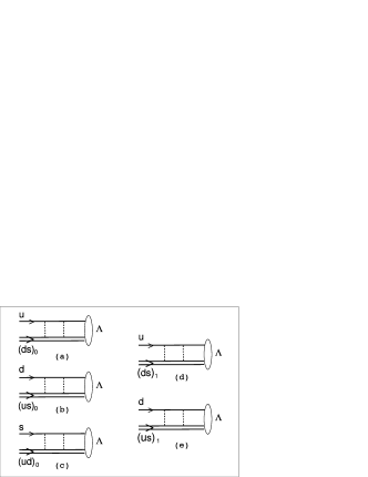
Figure 2: Subprocesses of the $\Lambda^{0}$ photoproduction in the QRM. One group of them, $(a)$, $(b)$ and $(c)$, concerns the recombinations of quarks with scalar diquarks, $u$+$(ds)_{0}$, $d$+$(us)_{0}$ and $s$+$(ud)_{0}$, respectively, while another one, $(d)$ and $(e)$, refer to the recombinations of quarks with vector diquarks, $u$+$(ds)_{1}$ and $d$+$(us)_{1}$. The subscriptions denote the spin states.

Applying of Eqs. (1) and (2) to the $\Lambda^{0}$ photoproduction leads to the following formula for the polarization qrm2

$$P=\dfrac{\sum\limits_{i,j,k}\sum\limits_{l}R_{l}J_{D}^{lijk}}{\sum\limits_{i,j,k}\sum\limits_{l}J_{I}^{lijk}},$$ (3)

where $R_{l}$ are the free parameters, so that the corresponding sum is performed over the scalar ($l=0$) and vector ($l=1$) cases,

$$J_{D(I)}^{lijk}=G_{\Lambda}^{2}\otimes\sigma_{D(I)}^{l}\otimes f^{p}_{(q_{i}q_{j})_{l}}\otimes f^{\gamma}_{q_{k}}\otimes\Delta^{3}\otimes\Delta^{4}.$$ (4)

Here, $G_{\Lambda}$ is the light cone wave function of $\Lambda^{0}$ lapage ; $\sigma_{D}^{l}$ is the interference term surviving in the numerator of Eq. (2); $\sigma_{I}^{l}$ is the quantity proportional to the total probability in the denominator of the same equation; $f^{p}_{(q_{i}q_{j})_{l}}$ is the momentum distribution function of the $(q_{i}q_{j})_{l}$ diquark in the proton; $f^{\gamma}_{q_{k}}$ is the structure function of the photon. The sum over $i,j,k$ is rather symbolic and includes only the appropriate combinations of quarks and diquarks to form the final $\Lambda^{0}$ (see Fig. 2).

Note that, in the QRM, the distribution functions are factorized into longitudinal and transverse momentum distribution parts as

$$f(r_{k})=f(x_{k},y_{k},z_{k})=f(x_{k})e^{-(y_{k}^{2}+z_{k}^{2})}.$$ (5)

Having taken the transverse parts of all the functions to have the same Gaussian form, we discuss henceforth the longitudinal those.

III Calculations and results

We present here the results of the QRM calculations of the $\Lambda^{0}$ polarization in photoproduction at $x_{F}>0$.

We used the Eqs. (3)-(4). Explicit expressions for $\sigma_{D(I)}^{l}$ as well as the parameter values were taken from Ref. qrm1 . It should be emphasized that all the parameters have been fixed for consistent fitting of the polarization in a variety of hadron-hadron reactions. Thus, for the $u$+$(ds)_{0}$, $d$+$(us)_{0}$ and $s$+$(ud)_{0}$ cases we took $R_{0}=2.5$ GeV, and for the $u$+$(ds)_{1}$, $d$+$(us)_{1}$ it was $R_{1}=-5.6$ GeV.

The photon structure function $f^{\gamma}_{q_{k}}$ plotted in the upper panel of Fig. 3 is taken from Ref. reya , the probabilities to find $u$, $d$ and $s$ quarks in the photon (up to a factor which does not affect the results since we deal with the ratio (3)) are given by the dotted, dashed and solid lines, respectively. For the diquark distribution functions of the proton $f_{(q_{i}q_{j})_{l}}^{p}$ we adopted those from Ref. ekelin shown in the lower panel of Fig. 3. We assumed that the functions for scalar and vector diquarks coincide (solid line) except for $(ud)_{0}$ (dashed line) due to the valence character of both $u$ and $d$ quarks forming it. Note that the functions depend on the momentum transfer squared and we have taken them at $Q^{2}=8$ GeV².

Figure 3: Upper panel: The photon structure function. The probabilities to find $u$ quark (dotted line), $d$ quark (dashed line) and $s$ quark (solid line) in the photon at $Q^{2}=8$ GeV² reya . Lower panel: Diquark distribution functions of the proton. The probabilities to find $(ds)_{0,1}$ and $(us)_{0,1}$ in the proton are assumed to be the same (solid line) except for $(ud)_{0}$ (dashed line) ekelin .

We have chosen the masses of quarks to be the following $m_{u}=m_{d}=0.3$ GeV, $m_{s}=0.55$ GeV, those of diquarks being simply the sums of the corresponding quark masses, i.e. $m_{(us)_{0,1}}=m_{(ds)_{0,1}}=m_{u}+m_{s}=0.85$ GeV and $m_{(ud)_{0}}=0.6$ GeV. Other fixed quantities of the QRM are the confinement scale parameter $\beta$=0.5 GeV in the $\Lambda^{0}$ light cone wave function and a parameter $p_{t}=0.3$ GeV, which fixed the transverse momentum distribution of the partons.

The calculated $p_{T}$ dependence of the polarization in the range 0.1 GeV $\leq p_{T}\leq$ 1.0 GeV is shown in Fig. 4 at $x_{F}=0.1$ (solid line), $x_{F}=0.2$ (dotted line) and $x_{F}=0.4$ (dashed line). First of all, one can see the polarization turn out to be positive. It grows more rapidly at lower $p_{T}$’s reaching approximate plateaus at about $p_{T}=0.6$ GeV, which is more distinctly manifested at $x_{F}=0.1$. The polarization decreases as one considers the higher $x_{F}$’s. It is seen that the calculations are in a good agreement with the HERMES data at $\zeta>0.25$ (solid points). The definition of the variable $\zeta$ will be given later.

The calculated $x_{F}$ dependence in the range $0.1\leq x_{F}\leq 0.5$ is presented in the upper panel of Fig. 5 at $p_{T}=0.5$ GeV (dotted line), $p_{T}=0.7$ GeV (dashed line) and $p_{T}=1.0$ GeV (solid line). One can see that the lines corresponding to the three values of $p_{T}$ fall slowly as $x_{F}$ increases up to about $x_{F}=0.34$, being, herewith, very close one to other. Afterwards, the line concerning $p_{T}=0.5$ GeV branches off the common trend and continues to fall while the rest those begin weakly to rise.

In Fig. 4 we have demonstrated how these calculations related to the HERMES measurements on the $\Lambda^{0}$ polarization in quasi-real photoproduction, which seem to be more suitable for this purpose Greb . However, we should make at this point a few comments. For some peculiarities of the HERMES experiment, the data are collected not as the traditional $x_{F}$ dependence but as the dependence on $\zeta=(E_{\Lambda}+p_{L\Lambda})/(E_{b}+p_{Lb})$, additionally integrated over $p_{T}$ ($E_{b}$ and $p_{Lb}$ are the energy and longitudinal momentum of the beam particle). Unlike $x_{F}$, the variable $\zeta$ is, thus, just an approximate measure of whether the hyperons were produced in the current or target fragmentation regions. Hence there is some ambiguity in the correlation between $x_{F}$ and $\zeta$, which causes an arbitrariness in the comparison of the HERMES data with results expressed in terms of $x_{F}$. The experimental $p_{T}$ dependence is also collected integrally over $\zeta$ for two regions, $\zeta\leq 0.25$ and $\zeta>0.25$. Additionally, the intermediate quasi-real photons of HERMES were not, certainly, monoenergetic, though this problem could be omitted by exploiting the fact that the polarization is incident particle energy independent.

To make the comparison with the experiment more correct, we have averaged the calculated $x_{F}$ dependence of the polarization over the $p_{T}$ distribution of $\Lambda^{0}$ hyperons produced at HERMES ptdistr . We show thus obtained results in the lower panel of Fig. 5 (solid line) in comparison with the experimental $\zeta$ dependence of the $\Lambda^{0}$ polarization (solid points). We used only the HERMES events at $\zeta>0.25$ because they more adequately relate to the $x_{F}>0$ region. One can see that the calculations sufficiently reproduce the experimental events.

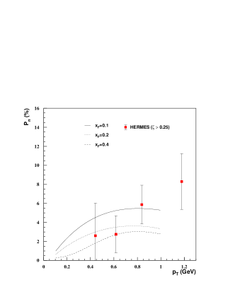
Figure 4: The calculated dependence of the $\Lambda^{0}$ polarization on $p_{T}$ at $x_{F}=0.1$ (solid line), $x_{F}=0.2$ (dotted line) and $x_{F}=0.4$ (dashed line) in comparison with the HERMES data from Ref. Greb (solid points).

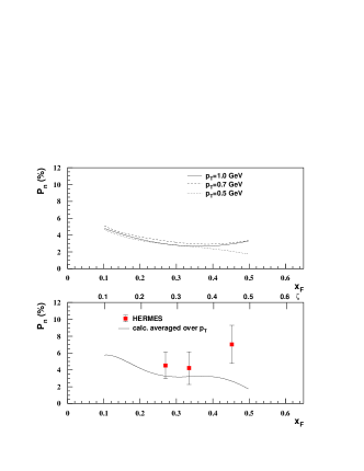
Figure 5: Upper panel: The calculated dependence of the $\Lambda^{0}$ polarization on $x_{F}$ at $p_{T}=0.5$ GeV (dotted line), $p_{T}=0.7$ GeV (dashed line) and $p_{T}=1.0$ GeV (solid line). Lower panel: The calculated dependence of the $\Lambda^{0}$ polarization on $x_{F}$ averaged over the $p_{T}$ distribution of $\Lambda^{0}$’s produced at HERMES (solid line) in comparison with the experimental dependence on $\zeta$ (solid points). The data are taken from Ref. Greb .

IV Summary and discussion

Following the recipes given in Refs. qrm1 ; qrm2 , we have shown that the transverse $\Lambda^{0}$ polarization in inclusive photoproduction at $x_{F}>0$ can be fairly accommodated by the quark recombination model, which comes, thus, outside of the reactions induced by hadrons. All the free parameters we used in the calculations have been already fixed to reproduce the polarization in other hadron-hadron interactions.

We have calculated as well the $p_{T}$ dependence of the polarization at $x_{F}=0.1$, $x_{F}=0.2$ and $x_{F}=0.4$ in the range 0.1 GeV $\leq p_{T}\leq$ 1.0 GeV as the dependence on $x_{F}$ at three fixed values of $p_{T}$, $p_{T}=0.5$ GeV, $p_{T}=0.7$ GeV, $p_{T}=1.0$ GeV in the range 0.1 $\leq x_{F}\leq$ 0.5.

We have compared the results with the HERMES data and discussed in what extent it could be suitable for this purpose. It was stressed that there is some ambiguity between the data and the results expressed in terms of $x_{F}$. To obtain results, which could be more correctly comparable with the experiment, we have averaged the calculated $x_{F}$ dependence over the $p_{T}$ distribution of $\Lambda^{0}$ hyperons produced at HERMES. Additionally, we used only the events of $\zeta>0.25$ to be, more or less, ensured that we dealt with the region of $x_{F}>0$. So, we have found a sufficient agreement with the data both in magnitude and in the sign of the polarization. However, this consistency can be regarded only as qualitative because of, at least, a few reasons. The uncertainties associated with the correlations between $\zeta$ and $x_{F}$ still remain. The intermediate photons emitted by the HERMES positron beam were not, indeed, monoenergetic. No information on the momentum transfer squared was derivable at the experiment while the structure functions used here are $Q^{2}$ dependent.

There are also another problems. Since the spin dependent distributions of the partons were not available, we have naively assumed the structure functions to have the same form as well for the scalar as for vector diquarks. We have also supposed that the subprocesses $s$+$(ud)_{0}$, $d$+$(us)_{0}$ and $u$+$(ds)_{0}$ contributed in the polarization with the same, positive, sign. These cases are structurally similar to the $K^{-}\rightarrow\Lambda^{0}$, $\pi^{-}\rightarrow\Lambda^{0}$ and $K^{+}\rightarrow\Lambda^{0}$ transitions, respectively. Certainly, the positive sign has been very reliably determined for $K^{-}\rightarrow\Lambda^{0}$, while, in fact, for the rest two cases the related situation is controversial due to the error bars of the data are still large (see also discussion in Ref. qrm1 ). In this light, it would be interesting to compare our results with those from Ref. suzuki , where similar calculations have been carried out.

We did not take here contributions from the heavier resonances into account, which are presumably significant for the $\Lambda^{0}$ polarization gatto ; long1 ; th4 ; liang . It can be done as a further improvement of the calculations, but, for this purpose, one needs to know, at least, the evolution of the variables $x_{F}$ and $p_{T}$ in the transition processes from the resonances to the final $\Lambda^{0}$.

It seems to be attractive to find the explicit expressions of the QRM amplitudes specifying the potential by the color field th3 , which might lead, in some sense, to a unification of the present approach with other quark scattering models swed ; gago .

We would like to thank K. Suzuki for providing useful information on the quark recombination model.

*

Appendix A

We present here some steps of the calculations in more explicit form.

The convolution in Eq. (4) is defined by

$$J_{D(I)}^{lijk}=G_{\Lambda}^{2}\otimes\sigma_{D(I)}^{l}\otimes f^{p}_{(q_{i}q_{j})_{l}}\otimes f^{\gamma}_{q_{k}}\otimes\Delta^{3}\otimes\Delta^{4}\\ =\int\left[\prod\limits_{m=1}^{4}\dfrac{dx_{m}dy_{m}dz_{m}}{x_{m}}\right]G_{\Lambda}^{2}\,\sigma_{D(I)}^{l}\,f^{p}_{(q_{i}q_{j})_{l}}\,f^{\gamma}_{q_{k}}\,\Delta^{3}\,\Delta^{4},$$ (6)

so that the integral is 12-dimensional.

According to Ref. qrm1 , we take

$$\Delta^{3}=\delta(x_{F}x_{4}+x_{F}x_{3}-x_{F})\\ \times\delta(y_{4}+y_{3}-P_{T}/p_{t})\delta(z_{4}+z_{3}),$$ (7)

$$\Delta^{4}=\delta(x_{F}x_{3}+x_{F}x_{4}-x_{1}-x_{2})\delta(y_{3}+y_{4}-y_{1}-y_{2})\\ \times\delta(z_{3}+z_{4}-z_{1}-z_{2})\delta\left(E_{Tf}-E_{Ti}\right),$$ (8)

where $P_{T}$ is the transverse momentum of $\Lambda^{0}$, $p_{t}$ is a normalization parameter to fix the transverse momentum distribution of the partons,

$$E_{Tf}=\dfrac{(y^{2}_{3}+z^{2}_{3})p^{2}_{t}+m^{2}_{q}}{x_{F}x_{3}}+\dfrac{(y^{2}_{4}+z^{2}_{4})p^{2}_{t}+m^{2}_{(qq)}}{x_{F}x_{4}},$$

$$E_{Ti}=\dfrac{(y^{2}_{1}+z^{2}_{1})p^{2}_{t}+m^{2}_{q}}{x_{1}}+\dfrac{(y^{2}_{2}+z^{2}_{2})p^{2}_{t}+m^{2}_{(qq)}}{x_{2}}.$$

We realized the condition when all the hyperons would be produced in the $x_{F}>0$ region by formal introducing the step function $\theta(x_{1}-x_{2})$, which simply means that each quark coming from the photon will be faster than the corresponding picked up diquark.

Let us rewrite Eq. (6) as

$$J=\int\left[\prod\limits_{m=1}^{4}{dx_{m}dy_{m}dz_{m}}\right]F(r_{1},r_{2},r_{3},r_{4})\Delta^{3}\Delta^{4},$$ (9)

where

$$F(r_{1},r_{2},r_{3},r_{4})=\dfrac{G_{\Lambda}^{2}\,\sigma_{D(I)}^{l}\,f^{p}_{(q_{i}q_{j})_{l}}\,f^{\gamma}_{q_{k}}}{x_{1}x_{2}x_{3}x_{4}}\,\theta(x_{1}-x_{2}).$$ (10)

To concentrate the attention on the integration over the momentum fractions $r_{m}=(x_{m},y_{m},z_{m})$, we introduced the denotation (10). For the same reason, the dependences on the rest parameters and indices are omitted.

We reduced the 12-dimensional integral to 5-dimensional one by using the delta functions (7) and (8).

Thus, an integration over $x_{1},x_{2},y_{1},y_{3},z_{1},z_{3}$ leads to the following substitutions in Eq. (10)

$$h=\left\{\begin{aligned} x_{1}=x_{F}-x_{2}\\ x_{3}=1-x_{4}\\ y_{1}=\dfrac{P_{T}}{p_{t}}-y_{2}\\ y_{3}=\dfrac{P_{T}}{p_{t}}-y_{4}\\ z_{1}=-z_{2}\\ z_{3}=-z_{4}.\end{aligned}\right.$$ (11)

Using the remaining delta-function $\delta\left(E_{Tf}-E_{Ti}\right)$, we integrated over $z_{4}$ as follows

$$J=\left.\dfrac{1}{x_{F}}\int\dots dz_{4}F(\dots,z_{4})\right|_{h}\delta(az_{4}^{2}-b),$$ (12)

where $h$ denotes the conditions (11),

$$a=\frac{p_{t}^{2}}{x_{F}x_{4}(1-x_{4})},$$ (13)

$$b=\frac{((\frac{P_{T}}{p_{t}}-y_{2})^{2}+z^{2}_{2})p^{2}_{t}+m^{2}_{q}}{x_{F}-x_{2}}+\frac{(y^{2}_{2}+z^{2}_{2})p^{2}_{t}+m^{2}_{(qq)}}{x_{2}}\\ -\frac{(\frac{P_{T}}{p_{t}}-y_{4})^{2}p^{2}_{t}+m^{2}_{q}}{x_{F}(1-x_{4})}-\frac{y_{4}^{2}p^{2}_{t}+m^{2}_{(qq)}}{x_{F}x_{4}}.$$ (14)

Applying the well known property of the delta-function one can write that

$$\delta(az_{4}^{2}-b)=\frac{1}{2}\sqrt{\frac{1}{ab}}\left[\delta\left(z_{4}-\sqrt{\frac{b}{a}}\right)+\delta\left(z_{4}+\sqrt{\frac{b}{a}}\right)\right].$$ (15)

Finally, after the integration over $z_{4}$, the Eq. (12) is split into a sum of integrals to be calculated numerically,

$$J=J^{+}+J^{-},$$ (16)

where

$$J^{\pm}=\dfrac{1}{2x_{F}}\int\limits_{\varepsilon}^{\frac{x_{F}}{2}}dx_{2}\int\limits_{\varepsilon}^{1-\varepsilon}dx_{4}\int\limits_{-\infty}^{\infty}dy_{2}\int\limits_{-\infty}^{\infty}dy_{4}\int\limits_{-\infty}^{\infty}dz_{2}\sqrt{\dfrac{1}{ab}}\\ \left.\frac{}{}\times F(r_{1},r_{2},r_{3},r_{4})\right|_{\stackrel{{\scriptstyle h}}{{z_{4}}}=\pm\sqrt{\frac{b}{a}}}.$$ (17)

The integration limit $\dfrac{x_{F}}{2}$ arose due to the step-function in Eq. (10), $\varepsilon$ is introduced because of the difficulties associated with the irregular behavior of the integrand at the borders of the integration regions over $x_{2}$ and $x_{4}$. In the actual computations, we have taken $\varepsilon=0.01$.

References

- (1) G. Bunce et al., Phys. Rev. Lett. 36, 1113 (1976).
- (2) K. Heller et al., Phys. Lett. B 68, 480 (1977).
- (3) L. G. Pondorm, Phys. Rep. 122, 57 (1985).
- (4) B. Lundberg et al., Phys. Rev. D 40, 3557 (1989).
- (5) S. Erhan et al., Phys. Lett. B 82, 301 (1979).
- (6) F. Abe et al., Phys. Rev. Lett. 50, 1102 (1983).
- (7) A. M. Smith et al., Phys. Lett. B 185, 209 (1987).
- (8) S. A. Gourly et al., Phys. Rev. Lett. 56, 2244 (1986).
- (9) I. V. Ajinenko et al., Phys. Lett. B 121, 183 (1983).
- (10) M. L. Faccini-Turluer et al., Z. Phys. C 1, 19 (1979).
- (11) J. Bensinger et al., Phys. Rev. Lett. 50, 313 (1983).
- (12) K. Heller et al., Phys. Rev. Lett. 51, 2025 (1983).
- (13) R. Rameika et al., Phys. Rev. D 33, 3172 (1986).
- (14) L. H. Trost et al., Phys. Rev. D 40, 1703 (1989).
- (15) J. Duryea et al., Phys. Rev. Lett. 67, 1193 (1991).
- (16) C. Wilkinson et al., Phys. Rev. Lett. 46, 803 (1981).
- (17) C. Ankenbrandt et al., Phys. Rev. Lett. 51, 863 (1983).
- (18) C. Wilkinson et al., Phys. Rev. Lett. 58, 855 (1987).
- (19) A. Morelos et al., Phys. Rev. Lett. 71, 2172 (1993).
- (20) E. C. Dukes et al., Phys. Lett. B 193, 135 (1987).
- (21) L. Deck et al., Phys. Rev. D 28, 1 (1983).
- (22) Y. W. Wah et al., Phys. Rev. Lett. 55, 2551 (1985).
- (23) M. I. Adamovich et al., Z. Phys. A 350, 379 (1995).
- (24) for reviews of experimental status and existing models, see A. D. Panagiotou, Int. J. Mod. Phys. A5, 1197 (1990). J. Soffer, hep-ph/9911373. S. M. Troshin, N. E. Tyurin, hep-ph/0201267
- (25) B. Andersson, G. Gustafson and G. Ingelman, Phys. Lett. B 85, 417 (1979).
- (26) T. A. DeGrand and H. I. Miettinen, Phys. Rev. D 23, 1227 (1981).
- (27) J. Szwed, Phys. Lett. B 105, 403 (1981).
- (28) J. M. Gago R. V. Mendes and P. Vaz, Phys. Lett. B 183, 357 (1987).
- (29) S. Soffer and N. A. Törngvist, Phys. Rev. Lett. 68, 907 (1992).
- (30) C. Boros, Liang Zuo-tang and Meng Ta-chung, Phys. Rev. Lett. 70, 1751 (1993).
- (31) W. G. D. Dharmaratna and G. R. Goldstein, Phys. Rev. D 53, 1073 (1996).
- (32) Y. Yamamoto, K.-I. Kubo and H. Toki, Prog. Theor. Phys. 98, 95 (1997).
- (33) N. Nakajima, K. Suzuki, H. Toki and K.-I. Kubo, hep-ph/9906451.
- (34) M. Anselmino, D. Boer, U. D’Alesio and F. Murgia, Phys. Rev. D 63, 054029 (2001).
- (35) Dong Hui and Liang Zuo-tang, Phys. Rev. D 70, 014019 (2004).
- (36) G. Gustafson and J. Hkkinen, Phys. Lett. B 303, 350 (1993).
- (37) C. Boros and Liang Zuo-tang, Phys. Rev. D 57, 4491 (1998).
- (38) ALEPH Collaboration, D. Buskulic et al., Phys. Lett. B 374, 319 (1996).
- (39) OPAL Collaboration, K. Ackerstaff et al., Eur. Phys. J. C 2, 49 (1998).
- (40) CERN-WA-004 Collaboration, D. Aston et al., Nucl. Phys. B195, 189 (1982).
- (41) SLAC-BC-072 Collaboration, K. Abe et al., Phys. Rev. D 29, 1877 (1984).
- (42) HERMES Collaboration, A. Airapetian et al., arXiv:0704.3133v1 [hep-ex].
- (43) K. P. Das and R. C. Hwa, Phys. Lett. B 68, 459 (1977).
- (44) R. C. Hwa, Phys. Rev. D 22, 1593 (1980).
- (45) M. Glück, E. Reya and A. Vogt, Phys. Rev. D 45, 3986 (1992).
- (46) G. P. Lepage and S. J. Brodsky, Phys. Rev. D 22, 2157 (1980).
- (47) S. Ekelin and S. Fredrikson, Phys. Lett. B 162, 373 (1985).
- (48) A. W. McKinley and H. Feshbach, Phys. Rev. 74, 1759 (1948).
- (49) R. H. Dalitz, Proc. R. Soc. (London) A206, 509 (1951).
- (50) K.-I. Kubo, K. Suzuki, hep-ph/0505179.
- (51) HERMES Collaboration, S. Belostotski, O. Grebenyuk and Yu. Naryshkin, Acta Phys. Polon. B 33, 3785 (2002).
- (52) R. Gatto, Phys. Rev. 109, 610 (1958).
- (53) Liang Zuo-tang and Liu Chun-xiu, Phys. Rev. D 66, 057302 (2002).