1. Introduction

This note describes a scheme for rapidly solving the systems of linear equations arising from the finite element or finite difference discretization of elliptic partial differential equations in two dimensions. Unlike most existing fast schemes which rely on iterative solvers (GMRES / conjugate gradient / …), the method described here directly inverts the matrix of the linear system. This obviates the need for customized pre-conditioners, and leads to dramatic speed-ups in environments in which the same equation needs to be solved for a sequence of different right-hand sides.

The scheme is described for the case of equations defined on a uniform square grid. Slight modifications would enable the handling of uniform grids on fairly regular two-dimensional domains, but further work would be required to construct methods for non-uniform grids or complicated geometries.

For a system matrix of size $N\times N$ (corresponding to a $\sqrt{N}\times\sqrt{N}$ grid), the scheme requires $O(N\log^{2}N)$ arithmetic operations, and $O(N\log N)$ storage to compute the full inverse. For a single solve, only $O(\sqrt{N}\,\log N)$ storage is required. Moreover, for problems loaded on the boundary only, any solves beyond the first require only $O(\sqrt{N}\,\log N)$ arithmetic operations (provided that only the solution on the boundary is sought). Numerical experiments indicate that the constants in these asymptotic estimates are quite moderate. For instance, to directly solve a system involving a $1\,000\,000\times 1\,000\,000$ matrix to seven digits of accuracy takes about four minutes on a 2.8GHz desktop PC with 512Mb of memory. Additional solves beyond the first can be performed in 0.03 seconds (provided only boundary data is involved).

The scheme is inspired by earlier work by Hackbusch and co-workers [hackbusch, H2_matrix, hackbusch2003, bebendorf2003] and work by Gu and Chandrasekaran [chan_gu_2001, chan_gu_2003, gu_SSS, HSS_sparse]. These authors have published methods that rapidly perform algebraic operations (matrix-vector multiplies, matrix-matrix multiplies, matrix inversion, etc) on matrices whose off-diagonal blocks have low rank. Our scheme is similar, but uses simpler data structures.

The fast inversion scheme retains its $O(N\log^{2}N)$ computational complexity for a wide range of network matrices. It does not rely on the fact that the matrix is associated with a PDE; rather, it works for any matrix whose inverse has off-diagonal blocks of low rank (what Hackbusch calls an $\mathcal{H}$-matrix, and Gu and Chandrasekaran calls an “HSS-matrix”).

The paper is structured as follows: Section 2 describes some known algorithms for performing fast operations on matrices with off-diagonal blocks of low rank. Section 3 describes a very simple $O(N^{2})$ inversion scheme. Section 4 describes how the $O(N^{2})$ scheme of Section 3 can be accelerated to $O(N\log^{2}N)$ using the methods of Section 2. Section 6 give the results of numerical experiments.

2. Preliminaries

In this section, we summarily describe a class of matrices for which there are known algorithms for rapidly evaluating the result of algebraic operations such as matrix-vector products, matrix-matrix products, and matrix inversions. The basic concept is that the off-diagonal blocks of the matrix can, to within some preset accuracy $\varepsilon$, be approximated by low-rank matrices. Different authors have given different definitions, and provided different algorithms; we mention that Hackbusch refers to such matrices as $\mathcal{H}$-matrices [hackbusch], or $\mathcal{H}^{2}$-matrices [H2_matrix], while Gu and Chandrasekaran refers to them as “Hierarchically Semi-Separable” (HSS) matrices [HSS_sparse] or “Sequentially Semi-Separable” (SSS) matrices [gu_SSS].

In this paper we will use the term HSS matrix to refer to an $n\times n$ matrix $B$ that can be tessellated in the pattern shown in Figure 2.1 in such a way that the rank of every block in the tessellation is bounded by some fixed small number $p$. Such a matrix can clearly be stored in $O(p\,n\log n)$ storage, and can be applied to a vector in $O(p\,n\log n)$ arithmetic operations. Moreover, via a trivial recursion (described in Appendix A), it is possible to invert such a matrix in $O(p\,n\log^{2}n)$ operations.

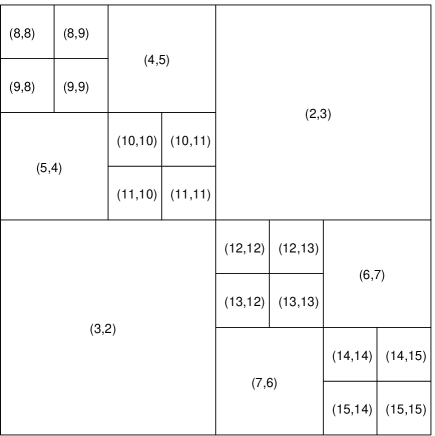
Figure 2.1. Tessellation of an HSS matrix.

Remark 2.1.

We will in this paper not distinguish between a matrix that is exactly an HSS-matrix, and a matrix that can to high precision be approximated by an HSS-matrix.

Remark 2.2.

We use the term SSS-matrix to refer to a matrix that is an HSS-matrix but has the additional property the bases for the row and column spaces of the off-diagonal blocks can be expressed hierarchically. As an example, a basis for the column space of the block labeled $(4,5)$ is constructed from the bases for the column spaces of the blocks $(8,9)$ and $(9,8)$. An SSS-matrix requires only $O(N)$ storage, and can be applied to a vector in $O(N)$ operations. Matrix-inversion schemes for SSS-matrices are a big more complicated than HSS inversion schemes, but in some environments, $O(N)$ inversion schemes exist, see e.g. [m2003].

Remark 2.3.

In Hackbusch’s terminology, what we call an HSS-matrix roughly corresponds to an $\mathcal{H}$-matrix, and what we call an SSS-matrix, roughly corresponds to an $\mathcal{H}^{2}$-matrix. The tessellations used by Hackbusch are slightly different, though.

3. An exact $O(N^{2})$ inversion scheme

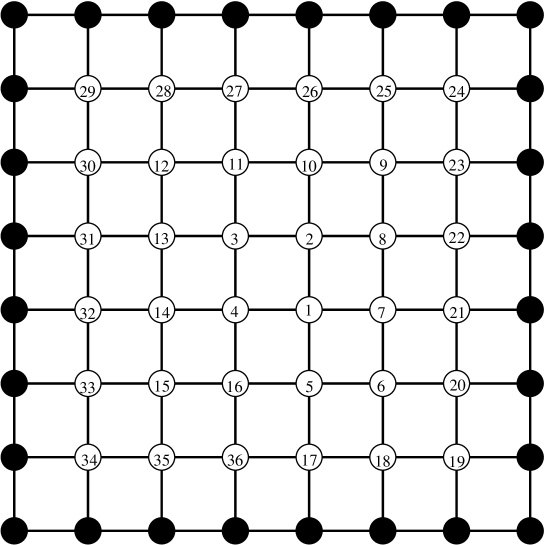
Figure 3.1. The computational grid for $n=6$.

Letting $n$ be a positive even integer, we consider a static conduction problem on a square $(n+2)\times(n+2)$ grid such as the one illustrated in Figure 3.1. Each interior node is connected to its four nearest neighbors with bars with positive conductivity. We prescribe the temperatures on the boundary nodes (marked with filled circles in Figure 3.1), and seek the equilibrium temperatures of the $N$ internal nodes, where $N=n^{2}$. This problem can be formulated as a linear system

(3.1) $$A\,x=b,$$

where $A$ is an $N\times N$ sparse matrix, $x$ is an $N\times 1$ vector of unknown temperatures, and $b$ is an $N\times 1$ vector derived from the pre-scribed boundary temperatures. When all bars have unit conductivity, the matrix $A$ in (3.1) is the well-known five-point stencil with coefficients $4$/$-1$/$-1$/$-1$/$-1$.

In this section we describe a method for directly solving the linear system (3.1) that relies on the sparsity structure of the matrix only. In the absence of rounding errors, it would be exact. When the matrix $A$ is of size $N\times N$, the scheme of this section requires $O(N^{2})$ floating point operations and $O(N)$ memory. This makes the scheme significantly slower than well-known $O(N^{3/2})$ schemes such as nested dissection. (We mention that $O(N^{3/2})$ is optimal in this environment.) The only purpose of the scheme presented in this section is that it can straight-forwardly be accelerated to an $O(N)$ or $O(N\log^{\kappa}N)$ scheme, as shown in Section 4.

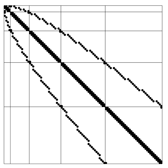
Figure 3.2. The sparsity pattern of $A$ in (3.1) for $N=100$.

Ordering the $N$ points in the grid in the spiral pattern shown in Figure 3.1, the matrix $A$ in equation (3.1) has the sparsity pattern shown in Figure 3.2. We next partition the grid into $n$ concentric squares, and collect the nodes into index sets $J_{1},\,J_{2},\,\dots\,,J_{n}$ accordingly. In other words,

$$\begin{array}[]{rcl}J_{1}&=&\{1,\,2,\,3,\,4\},\\ J_{2}&=&\{5,\,6,\,\dots\,,16\},\\ &\vdots&\\ J_{n}&=&\{(2n-1)^{2}+1,\,(2n-1)^{2}+2,\,\dots\,,(2n)^{2}\}.\end{array}$$

For $\kappa,\lambda\in\{1,\,2,\,\dots\,n\}$, we let $A_{\kappa\lambda}$ denote the submatrix of $A$ formed by the intersection of the $J_{\kappa}$ rows with the $J_{\lambda}$ columns. Then the linear system (3.1) takes on the block-tridiagonal form (also shown in Figure 3.2)

(3.2) $$\left[\begin{array}[]{cccccc}A_{11}&A_{12}&0&0&\cdots&0\\ A_{21}&A_{22}&A_{23}&0&\cdots&0\\ 0&A_{32}&A_{33}&A_{34}&\cdots&0\\ 0&0&A_{43}&A_{44}&\cdots&0\\ \vdots&\vdots&\vdots&\vdots&&\vdots\\ 0&0&0&0&\cdots&A_{nn}\end{array}\right]\,\left[\begin{array}[]{c}x_{1}\\ x_{2}\\ x_{3}\\ x_{4}\\ \vdots\\ x_{n}\end{array}\right]=\left[\begin{array}[]{c}b_{1}\\ b_{2}\\ b_{3}\\ b_{4}\\ \vdots\\ b_{n}\end{array}\right],$$

where $x$ and $b$ have been split accordingly.

The equation (3.2) can now easily be solved by eliminating the variables one by one. Using the first equation to eliminate $x_{1}$ from the second one, we obtain the following system of equations for the variables $x_{2},\dots,x_{n}$:

(3.3) $$\left[\begin{array}[]{cccccc}\tilde{A}_{22}&A_{23}&0&\cdots&0\\ A_{32}&A_{33}&A_{34}&\cdots&0\\ 0&A_{43}&A_{44}&\cdots&0\\ \vdots&\vdots&\vdots&&\vdots\\ 0&0&0&\cdots&A_{nn}\end{array}\right]\,\left[\begin{array}[]{c}x_{2}\\ x_{3}\\ x_{4}\\ \vdots\\ x_{n}\end{array}\right]=\left[\begin{array}[]{c}\tilde{b}_{2}\\ b_{3}\\ b_{4}\\ \vdots\\ b_{n}\end{array}\right],$$

where $\tilde{A}_{22}=A_{22}-A_{21}A_{11}^{-1}A_{12}$ and $\tilde{b}_{2}=b_{2}-A_{21}A_{11}^{-1}b_{1}$. The process used to eliminate $x_{1}$ can easily be continued to eliminate the first $n-1$ blocks. This leaves us with the $(8n-4)\times(8n-4)$ system

$$\tilde{A}_{nn}\,x_{n}=\tilde{b}_{n},$$

which we solve directly to obtain $x_{n}$. Once $x_{n}$ is known, we compute $x_{n-1}$ by solving the system

$$\tilde{A}_{n-1,n-1}\,x_{n-1}=\tilde{b}_{n-1}-A_{n-1,n}\,x_{n}.$$

The remaining $x_{j}$’s are computed analogously. The entire process is summed up in Algorithm I.

Algorithm 1: (1) $\tilde{A}_{11}=A_{11}$ and $\tilde{b}_{1}=b_{1}$. (2) for $\kappa=2:n$ (3) $\tilde{A}_{\kappa\kappa}=A_{\kappa\kappa}-A_{\kappa,\kappa-1}\,\tilde{A}_{\kappa-1,\kappa-1}^{-1}\,A_{\kappa-1,\kappa}$ (4) $\tilde{b}_{\kappa}=b_{\kappa}-A_{\kappa,\kappa-1}\,\tilde{A}_{\kappa-1,\kappa-1}^{-1}\,\tilde{b}_{\kappa-1}$ (5) end (6) $x_{n}=\tilde{A}_{nn}^{-1}\,\tilde{b}_{n}$ (7) for $\kappa=(n-1):(-1):1$ (8) $x_{\kappa}=\tilde{A}_{\kappa\kappa}^{-1}\,\bigl{(}\tilde{b}_{\kappa}-A_{\kappa,\kappa+1}\,x_{\kappa+1}\bigr{)}$ (9) end

Figure 3.3. This algorithm directly solves the tridiagonal system of equations (3.2).

We note that while all matrices $A_{\kappa\lambda}$ are sparse, the matrices $\tilde{A}_{\kappa\kappa}$ are dense. This means that the cost of inverting $\tilde{A}_{\kappa\kappa}$ in each step of Algorithm I is $O(\kappa^{3})$. (Note that the remaining matrix-matrix operations involve matrices that are diagonal or tri-diagonal and have negligible costs in comparison to the matrix inversion.) The total cost $T_{\rm total}^{\rm dense}$ is therefore

$$T_{\rm total}^{\rm dense}\sim\sum_{\kappa=1}^{n}\kappa^{3}\sim n^{4}\sim N^{2}.$$

Remark 3.1.

We note that the matrices $\tilde{A}_{\kappa\kappa}$ are not merely artificial objects of the numerical algorithm. In fact, $\tilde{A}_{nn}^{-1}$ is the matrix that maps the load on the boundary to the potential on the boundary. In many environments, the interior of the grid is unloaded (i.e. $b_{\kappa}=0$ when $\kappa=1,\,2,\dots,n-1$). In such cases, the operator $\tilde{A}_{nn}^{-1}$ is the solution operator of the original problem. Since none of the intermediate matrices $\tilde{A}_{\kappa\kappa}$ are required in this environment, the algorithm only requires $O(N)$ memory.

4. A fast direct solver

The computational cost of Algorithm I consists almost entirely of the inversion of the dense matrices $\tilde{A}_{\kappa\kappa}$. This cost can be greatly reduced whenever $\tilde{A}_{\kappa\kappa}$ is a “compressible” matrix in the sense described in Section 2. It is not the purpose of this paper to classify exactly when this happens; we will simply note that $A$ is typically compressible in this sense when it results from the discretization of an elliptic PDE, while it is typically not compressible when it results from the discretization of a highly oscillatory wave equation. We also note that the condition that $A$ result from the discretization of an elliptic PDE is very far from necessary, as the numerical examples in Section 6 demonstrate.

In cases where each $\tilde{A}_{\kappa\kappa}$ is what we in Section 2 called in “HSS”-matrix, very simple inversion schemes (see Appendix A) are available for computing an approximation to $\tilde{A}_{\kappa\kappa}^{-1}$ in $O(\kappa\,\log^{2}\kappa)$ arithmetic operations. The total computational cost of Algorithm I is then

$$T_{\rm total}^{\rm HSS}\sim\sum_{\kappa=1}^{n}\kappa\,(\log\kappa)^{2}\sim n^{2}\,(\log n)^{2}\sim N\,(\log N)^{2}.$$

This scheme requires $O(N\,\log N)$ memory to store the entire approximation to $A^{-1}$. Such a scheme has been implemented and the computational results are given in Section 6.

We note that the scheme is particularly memory efficient in environments where the domain is loaded on the boundary only, and only the solution at the boundary is sought, cf. Remark 3.1. In such situations, the operators $\tilde{A}_{\kappa\kappa}$ need not be stored, and the inversion algorithm only requires $O(\sqrt{N}\,\log N)$ memory. Moreover, if equation (3.1) is to be solved for several different right hand sides, subsequent solutions are obtained almost for free via application of the pre-computed operator $\tilde{A}_{nn}^{-1}$.

Finally we note that while it would require $O(N)$ memory to store $A$ itself, the scheme only accesses each entry of $A$ once. This means that these elements can either be computed on the fly (if given by a formula), or read sequentially from slow memory (“tape”).

Remark 4.1.

In cases where each Schur complement $\tilde{A}_{\kappa\kappa}$ is not only compressible in the “HSS”-sense, but also in the “SSS”-sense, the cost of approximately inverting $\tilde{A}_{\kappa\kappa}$ can be reduced from $O(\kappa^{3})$ to $O(\kappa)$, see Section 2. The total cost of Algorithm I is then

$$T_{\rm total}^{\rm SSS}\sim\sum_{\kappa=1}^{n}\kappa\sim n^{2}\sim N.$$

This is typically the case when $A$ results from the discretization of an elliptic partial differential equation.

5. Generalizations

The scheme presented here can in principle be adapted to more general grids in two and three dimensions. The generalization to other difference operators on uniform square grids is trivial. Other two-dimensional grids that are uniform in the sense that they can easily be partitioned into a sequence of concentric annuli can also quite easily be handled, and we expect the performance of such schemes to be similar to the performance reported in Section 6.

For grids arising from adaptive mesh-refinement, or involve more complex geometries, it is still possible to construct $O(N\log^{\kappa}N)$ inversion schemes; but they will very likely require algorithms involving a broader palette of operations on compressible matrices such as matrix-matrix multiplications. What is interesting about the specific method given here is that it requires only matrix-inversions and diagonal updates.

6. Numerical examples

The $O(N\log^{2}N)$ numerical scheme described in Sections 3 and 4 has been implemented and tested on a conduction problem on a square uniform grid. We assigned each bar in the grid a conductivity drawn from a uniform random distribution on the interval $[1,\,2]$. For a range of grid sizes between $50\times 50$ and $1\,000\times 1\,000$, we computed the operator $\tilde{A}_{n}^{-1}$ described in Section 3. The computational cost, the amount of memory required, and the accuracies obtained are presented in Table 6.1. The following quantities are reported:

$T_{\rm invert}$	Time required to construct $\tilde{A}_{n}$ (in seconds)
$T_{\rm apply}$	Time required to apply $\tilde{A}_{\rm n}$ (in seconds)
$M$	Memory required to construct $\tilde{A}_{n}$ (in kilobytes)
$e_{1}$	The largest error in any entry of $\tilde{A}_{n}^{-1}$
$e_{2}$	The error in $l^{2}$-operator norm of $\tilde{A}_{n}^{-1}$
$e_{3}$	The $l^{2}$-error in the vector $\tilde{A}_{nn}^{-1}\,r$ where $r$ is a unit vector of random direction.
$e_{4}$	The $l^{2}$-error in the first column of $\tilde{A}_{nn}^{-1}$.

We estimated $e_{1}$ and $e_{2}$ by comparing the result from the fast algorithm with the result from a brute force calculation of the Schur complement. We estimated $e_{3}$ and $e_{4}$ by solving equation (3.1) using iterative methods.

Some technical notes:

• The experiments were run on a 2.8GHz Pentium 4 PC with 512Mb of RAM.

• Off-diagonal blocks in the HSS-representations were represented to the fixed accuracy $\varepsilon=10^{-7}$.

• The ranks used in the off-diagonal blocks was allowed to vary from block to block (it was determined adaptively).

• The code used is written in a Matlab-FORTRAN hybrid. It is not at all optimized. Significant gains in efficiency should be obtainable by choosing block sizes in more intelligently than we did.

The scaling of $T_{\rm invert}$, $T_{\rm apply}$, and $M$ with $N$ is displayed in Figure 6.2. These tables appear to support our claims regarding the performance of the scheme. The values of $e_{1}$, $e_{2}$, $e_{3}$, and $e_{4}$ for different values of $N$ are shown in Figure 6.3. The table appears to indicate that errors grow as the square root of $N$ (in other words, linearly with the number of steps performed in Algorithm 1). This means that we could easily keep the error constant by very moderately increase $\varepsilon$ as the problem size gets larger.

Figure 6.4 gives the time $t_{\rm kappa}$ (in seconds) required to perform step $\kappa$ of the fast version of Algorithm 1. The large jumps in the curve correspond to repartitioning of the HSS-matrices. (The jaggedness of the curve gives an indication of how poorly optimized the code is.)

$N$	$T_{\rm invert}$	$T_{\rm apply}$	$M$	$e_{1}$	$e_{2}$	$e_{3}$	$e_{4}$
10000	5.93e-1	2.82e-3	3.82e+2	1.29e-8	1.37e-7	2.61e-8	3.31e-8
40000	4.69e+0	6.25e-3	9.19e+2	9.35e-9	8.74e-8	4.71e-8	6.47e-8
90000	1.28e+1	1.27e-2	1.51e+3	—	—	7.98e-8	1.25e-7
160000	2.87e+1	1.38e-2	2.15e+3	—	—	9.02e-8	1.84e-7
250000	4.67e+1	1.52e-2	2.80e+3	—	—	1.02e-7	1.14e-7
360000	7.50e+1	2.62e-2	3.55e+3	—	—	1.37e-7	1.57e-7
490000	1.13e+2	2.78e-2	4.22e+3	—	—	—	—
640000	1.54e+2	2.92e-2	5.45e+3	—	—	—	—
810000	1.98e+2	3.09e-2	5.86e+3	—	—	—	—
1000000	2.45e+2	3.25e-2	6.66e+3	—	—	—	—

Figure 6.1. Table summarizing the computational experiment described in Section 6.

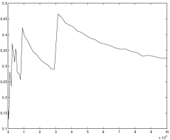
(a)	(b)	(c)

Figure 6.2. Plots of (a) $T_{\rm invert}/N$ versus $N$, (b) $T_{\rm apply}/\sqrt{N}$ versus $N$, (c) $M/\sqrt{N}$ versus $N$.

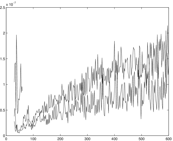
Figure 6.3. Plot of the errors versus the square root of the problem size $N$. The short top line on the left is $e_{2}$, the two lines extending to the right are $e_{3}$ and $e_{4}$, with $e_{4}$ on the top.

Figure 6.4. Plot of $t_{\kappa}$ versus $\kappa$.

Appendix A An $O(n\log^{2}n)$ inversion scheme for HSS-matrices

A recursive fast inversion scheme for HSS matrices follows immediately from the following formula for the inverse of a $2\times 2$ block matrix:

$$\left[\begin{array}[]{cc}A_{11}&A_{12}\\ A_{21}&A_{22}\end{array}\right]^{-1}=\\ \left[\begin{array}[]{cc}\bigl{(}A_{11}-A_{12}\,A_{22}^{-1}\,A_{21}\bigr{)}^{-1}&-\bigl{(}A_{11}-A_{12}\,A_{22}^{-1}\,A_{21}\bigr{)}^{-1}\,A_{12}\,A_{22}^{-1}\\ -A_{22}^{-1}\,A_{21}\,\bigl{(}A_{11}-A_{12}\,A_{22}^{-1}\,A_{21}\bigr{)}^{-1}&A_{22}^{-1}+A_{22}^{-1}\,A_{21}\,\bigl{(}A_{11}-A_{12}\,A_{22}^{-1}\,A_{21}\bigr{)}^{-1}\,A_{12}\,A_{22}^{-1}\end{array}\right]$$

From the formula, we immediately get Algorithm 2, displayed in Figure A.1. To see that this algorithm has complexity $O(n\log^{2}n)$, we note that the matrices $A_{12}$ and $A_{21}$ all have low rank. This means that the matrix-matrix multiplications that occur on lines (7) and (9) in fact consist simply of a small number of multiplications between HSS-matrices and vectors. Moreover, the matrix additions in lines (7) and (9) are in fact low-rank updates to HSS-matrices.

Algorithm 2: (1) function $B$ = invert HSS matrix($A$) (2) if ($A$ is “small”) then (3) $B=A^{-1}$ (4) else (5) Split $A=\left[\begin{array}[]{cc}A_{11}&A_{12}\\ A_{21}&A_{22}\end{array}\right]$. (6) $X_{22}$ = invert HSS matrix($A_{22}$) (7) $Y_{11}=A_{11}-A_{12}\,X_{22}\,A_{21}$ (8) $X_{11}$ = invert HSS matrix($Y_{11}$) (9) $B=\left[\begin{array}[]{cc}X_{11}&-X_{11}\,A_{12}\,X_{22}\\ -X_{22}\,A_{21}\,X_{11}&X_{22}+X_{22}\,A_{21}\,X_{11}\,A_{12}\,X_{22}\end{array}\right]$. (10) end if (11) end function

Figure A.1. Algorithm for inverting HSS matrices. Note that $A_{11}$, $A_{22}$, $X_{11}$, $X_{22}$, and $Y_{11}$ are all HSS-matrices, and that $A_{12}$ and $A_{21}$ are low-rank matrices.