Analogue to multiple electromagnetically induced transparency in all-optical drop-filter systems

Abstract

We theoretically study a parallel optical configuration which includes $N$ periodically coupled whispering-gallery-mode resonators. The model shows an obvious effect which has a direct analogy with the phenomenon of multiple electromagnetically induced transparency in quantum systems. The numerical simulations illuminate that the frequency transparency windows are sharp and highly transparent. We also briefly discuss the experimental feasibility of the current scheme in two practical systems, microrings and microdisks.

year number number identifier

Electromagnetically-induced transparency (EIT) Harris , which is based on the destructive quantum interference, is an interesting phenomenon that the absorption of a probe-laser field which is resonant with an atomic transition can be reduced or even eliminated by applying a strong driving laser beam at a different frequency. Since experimental observation in atomic vapors observation , this effect is playing an essential role in a variety of physical processes, ranging from lasing without inversion Zibrov , enhanced nonlinear optics Imamoglu to quantum computation and communication Lukin .

Recent theoretical analysis of optical coupled resonators (or cavities) without the use of atomic resonance have revealed that coherent effects in coupled resonator systems are remarkably similar to those in atoms. In Ref. smith , it was shown that the EIT-like effect can be established in directly coupled optical resonators due to mode splitting and classical destructive interference smith . In Ref. fan , it was pointed out that the existence of a classical analogue of the electromagnetically induced transparency in coupled optical resonators is crucial for on-chip coherent manipulation of light at room temperatures, including the capabilities of stopping, storing and time reversing an incident optical pulse. More recently, some experiments have been reported for observing the structure tuning of the EIT-like spectrum in a compound glass waveguide platform using relatively large resonators chu , coupled fused-silica microspheres naweed ; kouki and integrated micron-size silicon optical resonator systems xu . These experiments open up the new possibility for optical communication and simulation of coherent effect in quantum optics using multiple coupled optical resonators poon .

In this paper, we study multiple EIT-like transmission spectrum by means of $N$ indirectly coupled resonators (via two parallel waveguides, namely, bus and drop) which is a generalization of the two coupled resonators system maleki . $N$ indirectly coupled resonators result in $N-1$ frequency transparency windows with equal separation. The numerical simulations indicate that these frequency windows are ultra-sharp and highly transparent with practical parameters. The experimental feasibility of the current scheme in two practical systems, microrings and microdisks, will be finally discussed briefly.

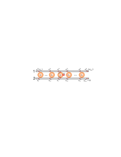
Figure 1: (Color online) Coupled microcavity resonators sharing two waveguides 1 and 2, namely, bus and drop. As a run-of-mill example, loss parameters in cavity i are detailedly described.

Consider an array of resonators in which each resonator is coupled to the adjacent resonators by means of two parallel waveguides, as shown in Fig. 1. The cavities are labeled in ascending order from left to right, and it is assumed that there are $N$ cavities altogether. In the case of slowly varying field amplitudes, the modes of this system can be described by the coupled harmonic oscillator model. The motion of the i-th ($\mathrm{i=1,2,...,N}$) cavity mode $a_{\text{{i}}}$ (with the center frequency $\omega_{\mathrm{i}}$) is

$$\frac{da_{\text{{i}}}}{dt} =i\left(\omega-\omega_{\mathrm{i}}\right)a_{\mathrm{i}}-\frac{\kappa_{\mathrm{0}}^{\mathrm{(i)}}+\kappa_{\mathrm{1}}^{\mathrm{(i)}}+\kappa_{\mathrm{2}}^{\mathrm{(i)}}}{2}a_{\mathrm{i}}$$

$$-\sqrt{\kappa_{\mathrm{1}}^{\mathrm{(i)}}}a_{\mathrm{i}}^{\mathrm{in}}-\sqrt{\kappa_{\mathrm{2}}^{\mathrm{(i)}}}e^{i\phi_{\mathrm{i}}}a_{\mathrm{i+1}}^{\mathrm{out}}.$$ (1)

Here $\omega$ denotes the carrier frequency of the input laser field; $\kappa_{\mathrm{0}}^{\mathrm{(i)}}$, $\kappa_{\mathrm{1}}^{\mathrm{(i)}}$ and $\kappa_{\mathrm{2}}^{\mathrm{(i)}}$ represent the linewidth associated with the intrinsic cavity losses, the coupling to waveguides 1 and 2, respectively; $a_{\mathrm{i}}^{\mathrm{in}}$ and $a_{\mathrm{i+1}}^{\mathrm{out}}$ describe the input fields of the i-th cavity from waveguides 1 and 2, respectively, as shown in Fig. 1. The two output fields (transmission and reflection) are related to the input fields by the output-input relations $a_{\mathrm{i}}^{\mathrm{in}}=\exp\left(i\phi_{\mathrm{i-1}}\right)\left(a_{\mathrm{i-1}}^{\mathrm{in}}+\sqrt{\kappa_{\mathrm{1}}^{\mathrm{(i)}}}a_{\mathrm{i-1}}\right)$ and $a_{\mathrm{i}}^{\mathrm{out}}=\exp\left(i\phi_{\mathrm{i}}\right)a_{\mathrm{i+1}}^{\mathrm{out}}+\sqrt{\kappa_{\mathrm{2}}^{\mathrm{(i)}}}a_{\mathrm{i}}$. Here $\phi_{\mathrm{i}}$ stands for the phase delay along the waveguides between the adjacent cavities i and i+1. For simplicity and convenience, we put $\exp\left(i\phi_{\mathrm{i}}\right)=1$ by choosing appropriate resonator-resonator distance $L$.

We are interested in the steady-state regime of the current system. To facilitate the discussion, we also suppose that each cavity has the same dissipation, which originate from the intrinsic loss and the two waveguides, i.e., $\kappa_{\mathrm{0}}^{\mathrm{(i)}}=\kappa_{\mathrm{0}}$, $\kappa_{\mathrm{1}}^{\mathrm{(i)}}=\kappa_{\mathrm{1}}$, $\kappa_{\mathrm{2}}^{\mathrm{(i)}}=\kappa_{\mathrm{2}}$. Neglecting all the fluctuations, setting $da_{\text{{i}}}/dt=0$, and taking the expectation value with respect to the steady state of Eq. (1), it is easy to find that

$$\left(i\Delta_{\mathrm{i}}-\frac{\kappa}{2}\right)\left\langle a_{\mathrm{i}}\right\rangle-\sqrt{\kappa_{\mathrm{1}}}\left\langle a_{\mathrm{i}}^{\mathrm{in}}\right\rangle-\sqrt{\kappa_{\mathrm{2}}}\left\langle a_{\mathrm{i+1}}^{\mathrm{out}}\right\rangle=0,$$ (2)

where $\kappa=\kappa_{\mathrm{0}}+\kappa_{\mathrm{1}}+\kappa_{\mathrm{2}}$ denotes the total dissipation of each cavity mode, and $\Delta_{\mathrm{i}}$ denotes the detuning $\omega-\omega_{\mathrm{i}}$. Also, using simple recurrence relations, we obtain $\left\langle a_{\mathrm{i}}^{\mathrm{in}}\right\rangle=\left\langle a_{\mathrm{in}}\right\rangle+\sqrt{\kappa_{\mathrm{1}}}\sum_{\mathrm{j=1}}^{\mathrm{i-1}}\left\langle a_{\mathrm{j}}\right\rangle$ and $\left\langle a_{\mathrm{i}}^{\mathrm{out}}\right\rangle=\sqrt{\kappa_{\mathrm{2}}}\sum_{\mathrm{j=i}}^{\mathrm{N}}\left\langle a_{\mathrm{j}}\right\rangle$, where we have used $\left\langle a_{\mathrm{1}}^{\mathrm{in}}\right\rangle=\left\langle a_{\mathrm{in}}\right\rangle$ and $\left\langle a_{\mathrm{N+1}}^{\mathrm{out}}\right\rangle=0$. Therefore, Eq. (2) reduces to

$$\left(i\Delta_{\mathrm{i}}-\frac{\kappa}{2}\right)\left\langle a_{\mathrm{i}}\right\rangle-\sqrt{\kappa_{\mathrm{1}}}\left\langle a_{\mathrm{in}}\right\rangle-\kappa_{\mathrm{1}}\sum_{\mathrm{j=1}}^{\mathrm{i-1}}\left\langle a_{\mathrm{j}}\right\rangle-\kappa_{\mathrm{2}}\sum_{\mathrm{j=i+1}}^{\mathrm{N}}\left\langle a_{\mathrm{j}}\right\rangle=0.$$ (3)

If $\kappa_{\mathrm{1}}=\kappa_{\mathrm{2}}$, Eq. (3) can be further simplified to

$$\left\langle a_{\mathrm{i}}\right\rangle=\frac{\sqrt{\kappa_{\mathrm{1}}}\left\langle a_{\mathrm{in}}\right\rangle+\kappa_{\mathrm{1}}\sum_{\mathrm{j=1}}^{\mathrm{N}}\left\langle a_{\mathrm{j}}\right\rangle}{i\Delta_{\mathrm{i}}-\kappa_{\mathrm{0}}/2}.$$ (4)

Through simple algebra, we achieve

$$\sum_{\mathrm{i=1}}^{\mathrm{N}}\left\langle a_{\mathrm{i}}\right\rangle=\frac{\sqrt{\kappa_{\mathrm{1}}}c}{1-\kappa_{\mathrm{1}}c}\left\langle a_{\mathrm{in}}\right\rangle,$$ (5)

where the constant $c=\sum_{\mathrm{i=1}}^{\mathrm{N}}\left(i\Delta_{\mathrm{i}}-\kappa_{\mathrm{0}}/2\right)^{-1}$. According to the output-input relations, the final output field which is our interest, can be expressed as

$$\left\langle a_{\mathrm{out}}\right\rangle=\left\langle a_{\mathrm{N+1}}^{\mathrm{in}}\right\rangle=\frac{1}{1-\kappa_{\mathrm{1}}c}\left\langle a_{\mathrm{in}}\right\rangle\text{,}$$ (6)

so the overall power transmission coefficient $\left|\mathcal{T}\left(\omega\right)\right|^{2}=\left|\left\langle a_{\mathrm{out}}\right\rangle/\left\langle a_{\mathrm{in}}\right\rangle\right|^{2}$ for this system reads

$$\left|\mathcal{T}\left(\omega\right)\right|^{2}=\left|1-\kappa_{\mathrm{1}}c\right|^{-2}.$$ (7)

Obviously, the transmission $\left|\mathcal{T}\left(\omega\right)\right|^{2}$ has $N$ local minima $\left|\mathcal{T}\left(\omega\right)\right|_{\min}^{2}$ $\left(\simeq 0\right)$ at $\omega\simeq\omega_{\mathrm{i}}$ and $N-1$ local maxima $\left|\mathcal{T}\left(\omega\right)\right|_{\max}^{2}$ at $\omega=\left(\omega_{\mathrm{i}}+\omega_{\mathrm{i+1}}\right)/2$. For the simplicity of numerical simulation, we further assume that the resonant frequencies are equally (or periodically) spaced between the adjacent cavities’ modes, i.e., $\omega_{\mathrm{i+1}}-\omega_{\mathrm{i}}=\delta$.

The overall transmission is shown in the red solid lines of Fig. 2(a)-2(f), which describe the cases of $N=1$, $2$, $3$, $4$, $5$, $6$, respectively. When $N=1$, i.e., the system only includes one cavity, Fig. 2(a) actually depicts the well-known transmission response curve of a single cavity mode rokhsari . When $N>1$, obviously, there exist some sharp peaks in the middle of the adjacent cavities’ modes, which is a direct analogy to the phenomenon of electromagnetically induced transparency in atomic vapors rmp  or semiconductors hailin . These narrow peaks originate from the interference effect of the cavities’ delay. The output $a_{\mathrm{i+1}}^{\mathrm{out}}$ of the i+1-th cavity couples back into the $\mathrm{i}$-th cavity as the second input port besides $a_{\mathrm{i}}^{\mathrm{in}}$. The transmission is nearly canceled when the light is resonant with one of the cavities’ modes due to the over-coupling regime ($\kappa_{\mathrm{1}},\kappa_{\mathrm{2}}\gg\kappa_{\mathrm{0}}$) between the waveguides and resonators rokhsari . However, in the middle the adjacent modes, the destructive interference results in a very narrow transmission resonance maleki . We will discuss these in the following part.

For comparison, the blue dotted lines in Fig. 2(b)-2(f) describe the cases that the output $a_{\mathrm{i+1}}^{\mathrm{out}}$ of the i+1-th cavity directly decays into free space instead of coupling back into the $\mathrm{i}$-th cavity. Therefore there is no interference effect between the two input fields, and the whole output transmission describes the collective response of all the cavities’ modes.

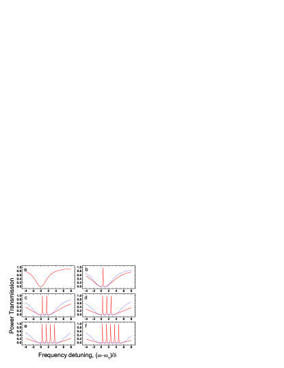
Figure 2: (Color online) Overall power transmission coefficient $\left|\mathcal{T}\left(\omega\right)\right|^{2}$. Red solid (blue dotted) lines in Figure 2(a)-2(f) describe the system including one, two, three, four, five, six cavities, respectively, and there are (no) side coupling among them. Other parameters: $\kappa_{\mathrm{0}}/\kappa_{\mathrm{1}}=10^{-3}$, $\kappa_{\mathrm{1}}/\delta=2$.

To quantitatively characterize the above optical EIT, Fig. 3(a) and 3(b) depict the full width at half maximum (FWHM) and maximal transmission rate of the EIT windows respectively. As shown in Fig. 3(a), FWHM mostly depends on the coupling strength $\kappa_{\mathrm{1}}$, that is, larger $\kappa_{\mathrm{1}}$ leads to narrower peak for the given intrinsic cavity loss $\kappa_{\mathrm{0}}$ and the mode spacing $\delta$. In other words, once the parameters $\kappa_{\mathrm{0}}$ and $\kappa_{\mathrm{1}}$ have been given, the smaller $\delta$ causes sharper peak. It agrees with the experiental prediction that there is no EIT phenomenon if $\kappa_{\mathrm{1}}\ll$ $\delta$, because at this time the spectrum differences between the adjacent cavities’ modes are so large that interference does not work significantly, and the total transmission will represent the resonant absorptions of $N$ cavities’ modes. Fig. 3(b) shows how the maximal transmission $\left|\mathcal{T}\left(\omega\right)\right|_{\max}^{2}$ depends on the intrinsic cavity loss $\kappa_{\mathrm{0}}$ for a given coupling strength $\kappa_{\mathrm{1}}$. When the magnitude of $\kappa_{\mathrm{0}}$ is of the order of$\ \delta$, $\left|\mathcal{T}\left(\omega\right)\right|_{\max}^{2}$ will decrease rapidly to zero; when $\kappa_{\mathrm{0}}$ can be arbitrarily small, $\left|\mathcal{T}\left(\omega\right)\right|_{\max}^{2}$ almost maintains unitary since there is no external loss for the optical resonator-waveguide system here.

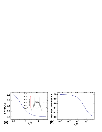
Figure 3: (Color online) (a) FWHM of the EIT windows vs. $\kappa_{\mathrm{1}}$. Other parameter: $\kappa_{\mathrm{0}}/\delta=10^{-4}$. (b) Maximal power transmission (peak value) $\left|\mathcal{T}\left(\omega\right)\right|_{\max}^{2}$ vs. $\kappa_{\mathrm{0}}$. Other parameter $\kappa_{\mathrm{1}}/\delta=2$.

It is necessary to give some brief remarks on the analogy and difference between the electromagnetically and coupled-resonator induced transparency. On one hand, the coupled-resonator induced transparency can be described in the language which is used in the thoroughly documented field of EIT, where the role of the “atom” is played by the cavity, the “atomic transition” is acted by the cavity mode, and the ”strong driving laser beam” is represented by the strong coupling between the adjacent cavities. As shown in Fig. 4, we illustrate the sketched level diagram of two coupled cavities, i.e., $N=2$. Due to the over-coupling regime among the waveguides and cavities, a probe beam tuned on near-resonance with the first cavity mode $a_{\mathrm{1}}$ will be strongly coupled into the second waveguide. The application of the second cavity mode $a_{\mathrm{2}}$ and the strong coupling between $a_{\mathrm{1}}$ and $a_{\mathrm{2}}$ will split the first cavity mode into two dressed modes $a_{\mathrm{1}}^{\prime}$ and $a_{\mathrm{1}}^{\prime\prime}$ with different energies. In this case, the input field with frequency $\omega_{\mathrm{1}}$ can enter into the second waveguide via two intermediate cavity modes, $a_{\mathrm{1}}^{\prime}$ and $a_{\mathrm{1}}^{\prime\prime}$, whose detunings are of equal magnitudes and opposite signs. As a result, their contributions to the second waveguide process cancel out in second-order perturbation theory and the first cavity becomes transparent to the probe beam. Remarkably, this is analogous to the conventional EIT in atomic medium.

On the other hand, unlike the conventional atomic EIT, the coupled-resonator induced transparency needs the condition that the probe beam be tuned on near-resonance but not exact-resonance with the cavity mode. This is because the system works in the over-coupling regime which results in the light transferring from waveguide 1 to 2 with near unit transfer efficiency. Thus the power transmission from waveguide 1 to the second cavity is very small and the returned power from the second to the first cavity is even smaller. As a result, the transmission will be nearly canceled when the light is resonant with the first cavity mode since the destructive interference does not play a significant role in the light transmission. For more cavities, similar treatments can be done, which lead to the above-mentioned multiple EIT-like transmission spectrum.

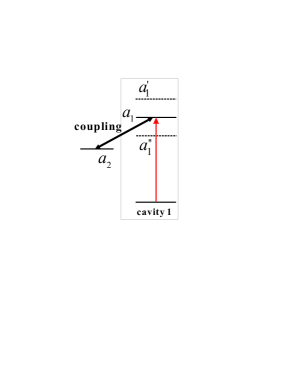
Figure 4: (Color online) Sketched level diagram of the first cavity coupled with the second. Double-arrow bold line describes the strong coupling between the adjacent cavities via two waveguides. $a_{\mathrm{1}}^{\prime}$ and $a_{\mathrm{1}}^{\prime\prime}$ are two dressed modes with different energies.

We now turn to analyze the experimental feasibility of the present multiple optical EIT. For this we briefly discuss two systems, microrings lipson ; xu and microdisks kipp . Recently, such cavities have been considered as candidates for quantum information processing buck ; brun ; xiao ; shen ; waks . For microring resonators, the adjacent rings can be linked by two etched waveguides, so the resonators (microrings) and data channels (waveguides) can be integrated on a chip. Modes in microrings posses high quality factors (up to $1.4\times 10^{5}$ niehusmann ) and ultra-small mode volumes. The current silicon-on-insulator (SOI) technology allows for a high etching precision (better than $0.02$ $\operatorname{\mu m}$) by designing the mask and controlling inductively-coupled-plasma reactive ion etching, so that the resonant detuning $\delta$ of the microrings and the condition $\exp\left(i\phi\right)=1$ are easily satisfied. For microdisk resonators, quality factors in excess of 1 million have been demonstrated in micron scale silicon nitride (SiN_x) painter and silica kipp at near visible wavelengths and in the $1550$-$\operatorname{nm}$ band, respectively. In-and-out coupling can be achieved by use of two fiber tapers rokhsari . To achieve and modulate the resonant detuning $\delta$, the microdisk modes can be first positioned with an accuracy of $0.5$ $\operatorname{nm}$ using standard lithographic techniques. For a more accurate modulation, wet chemical etching introduced in References xudong ; painter (better than $0.2$ $\operatorname{pm}$) and temperature tuning discussed in Reference temperature can be applied.

In conclusion, we theoretically present an all-optical scheme to directly simulate multiple EIT using periodically side-coupled $N$ resonators. The highly sharp EIT-like transparency windows only rely on the frequencies of the cavities’ modes, so that it is selective through the design of resonator array. This is of importance for applications in optical communications (e.g., channel-selective bandpass filters) and quantum information processing (e.g., slow light systems).

- (1) E. Arimondo, Progress in Optics 35, 259 (1996); S. E. Harris, Phys. Today 50, 37 (1997); J. P. Marangos, J. Mod. Opt. 45, 471 (1998); M. Fleischhauer, A. Imamoglu, and J. P. Marangos, Rev. Mod. Phys. 77, 633 (2005), and references therein.
- (2) S. E. Harris, J. E. Field, and A. Kasapi, Phys. Rev. A 46, R29 (1992); Y. Q. Li and M. Xiao, Phys. Rev. A 51, R2703 (1995); S. E. Harris and L. V. Hau, Phys. Rev. Lett. 82, 4611 (1999); A. V. Sokolov, D. R. Walker, D. D. Yavuz, G. Y. Yin, and S. E. Harris, Phys. Rev. Lett. 85, 562 (2000).
- (3) A. S. Zibrov et al., Phys. Rev. Lett. 75, 1499 (1995).
- (4) S. E. Harris, J. E. Field, and A. Imamoglu, Phys. Rev. Lett. 64, 1107 (1990); H. Schmidt and A. Imamoglu, Opt. Lett. 21, 1936 (1996); S. E. Harris and L. V. Hau, Phys. Rev. Lett. 82, 4611 (1999); M. D. Lukin and A. Imamoglu, Phys. Rev. Lett. 84, 1419 (2000).
- (5) M. D. Lukin, S. F. Yelin, and M. Fleischhauer, Phys. Rev. Lett. 84, 4232 (2000); M. D. Lukin and A. Imamoglu, Nature (London) 413, 273 (2001); Z. Ficek and S. Swain, J. Mod. Opt. 49, 3 (2002).
- (6) D. D. Smith, H. Chang, K. A. Fuller, A. T. Rosenberger, and R. W. Boyd, Phys. Rev. A 69, 063804 (2004).
- (7) M. F. Yanik, W. Suh, Z. Wang, and S. Fan, Phys. Rev. Lett. 93, 233903 (2004).
- (8) S. T. Chu, B. E. Little, W. Pan, T. Kaneko, and Y. Kokubun, IEEE Photonics Technol. Lett. 11, 1426 (1999).
- (9) A. Naweed, G. Farca, S. I. Shopova, and A. T. Rosenberger, Phys. Rev. A 71, 043804 (2005).
- (10) K. Totska, N. Kobayashi, and M. Tomita, Phys. Rev. Lett. 98, 213904 (2007).
- (11) Q. Xu, S. Sandhu, M. L. Povinelli, J. Shakya, S. Fan, and M. Lipson, Phys. Rev. Lett. 96, 123901 (2006); Q. Xu, J. Shakya, and M. Lipson, Opt. Express 14, 6463 (2006).
- (12) J. K. Poon, L. Zhu, G. A. DeRose, A. Yariv, Opt. Lett. 31, 456 (2006).
- (13) L. Maleki, A. B. Matsko, A. A. Savchenkov, and V. S. Ilchenko, Opt. Lett. 29, 626 (2004).
- (14) H. Rokhsari and K. J. Vahala, Phys. Rev. Lett. 92, 253905 (2004).
- (15) M. Fleischhauer, A. Imamoglu, and J. P. Marangos, Rev. Mod. Phys. 77, 633 (2005).
- (16) M. Phillips and H. Wang, Phys. Rev. Lett. 89, 186401 (2002).
- (17) V. R. Almeida, C. A. Barrios, R. R. Panepucci, and M. Lipson, Nature (London) 431, 1081 (2004).
- (18) T. J. Kippenberg, S. M. Spillane, D. K. Armani, and K. J. Vahala, Appl. Phys. Lett. 83, 797 (2003).
- (19) J. R. Buck and H. J. Kimble, Phys. Rev. A 67, 033806 (2003); S. M. Spillane et al., Phys. Rev. A 71, 013817 (2005); D. W. Vernooy and H. J. Kimble, Phys. Rev. A 55, 1239 (1997); T. Aoki, B. Dayan, E. Wilcut, W. P. Bowen, A. S. Parkins, H. J. Kimble, T. J. Kippenberg and K. J. Vahala, Nature 443, 671 (2006).
- (20) T. A. Brun and H. Wang, Phys. Rev. A 61, 032307 (2000).
- (21) W. Yao, R. B. Liu, and L. J. Sham, Phys. Rev. Lett. 95, 030504 (2005).
- (22) Y.-F. Xiao et al., Phys. Rev A 70, 042314 (2004); Y.-F. Xiao, Z.-F. Han, G.-C. Guo, Phys. Rev. A 73, 052324 (2006).
- (23) E. Waks and J. Vuckovic, Phys. Rev. Lett. 96, 153601 (2006).
- (24) J. Niehusmann et al., Opt. Lett. 29, 2861 (2004).
- (25) P. E. Barclay, K. Srinivasan, O. Painter, B. Lev, H. Mabuchi, eprint: quant-ph/0605234.
- (26) I. M. White, N. M. Hanumegowda, H. Oveys, and X. Fan, Opt. Express 13, 10754 (2005).
- (27) M. L. Gorodetsky and I. S. Grudinin, J. Opt. Soc. Am. B 21, 697 (2004).