Convergence properties of Donaldson’s $T$-iterations on the Riemann sphere

Abstract. In [Don05b] Donaldson gives three operators on a space of Hermitian metrics on a complex projective manifold: $T,T_{\nu},T_{K}.$ Iterations of these operators converge to balanced metrics, and these themselves approximate constant scalar curvature metrics. In this paper we investigate the convergence properties of these iterations by examining the case of the Riemann sphere as well as higher dimensional $\mathbb{CP}^{n}$.

1 Introduction

Let $X$ be a compact complex manifold with a positive holomorphic line bundle $L$. A long-standing open problem in Kähler geometry, building on Yau’s solution of the Calabi conjecture [Yau78], is to find sufficient conditions for the existence of a constant scalar curvature Kähler metric in $c_{1}(L)$. Another is as follows: can such a metric be obtained naturally as a limit of algebraic metrics via embeddings of $X$ into $\mathbb{P}\mathrm{H}^{0}(X,L^{k})$?

This idea of approximating Kähler metrics by restricting Fubini-Study metrics, advocated by Yau over the years, has led to the development of a rich theory relating analysis and notions of stability in the sense of geometry invariant theory (see [Yau93], [Tia90], [Tia97], [Don02]). In a fundamental paper, Donaldson [Don01] showed that, under an assumption on the space of automorphisms, the metrics induced from balanced embeddings [Zha96] of $X$ into projective space by sections of $L^{k}$ converge to the constant scalar curvature metric as $k\rightarrow\infty$. The balanced condition means that

$$\int_{X}\frac{Z_{i}\overline{Z_{j}}}{|Z|^{2}}\,d\mu\ =\ c\delta_{ij},$$

(where $d\mu$ is the volume form on $X$ induced by the Fubini-Study metric and $c$ is a constant depending on the data $(X,L^{k})$ and not on the particular embedding) and this is equivalent to the Chow stability of the embedding [Zha96], [Luo98], [PS03].

Recently [Don05a, Don05b], Donaldson has devised iterative procedures on the space of Hermitian metrics on $\mathrm{H}^{0}(X,L^{k})$ to find approximations to these balanced metrics. For sufficiently large $k$, these approximations are close to a constant scalar curvature metric. Explicit numerical computations, focused in the Calabi-Yau case where there are possible applications to string theory, have been obtained in [Don05b], [DKLR06b], [DKLR06a]. See also [HW06], [Kel07a], and [Rub07] where different methods are used.

Donaldson’s three iterative maps $T$, $T_{\nu}$, and $T_{K}$, described below, are interesting in their own right. Indeed, as pointed out in [Don05b], it is likely that these maps can be viewed as discrete approximations to the Ricci and Calabi flows.

Instead of pursuing general questions of existence, in this paper we pick a simple compact complex manifold – the Riemann sphere – and investigate the convergence properties of each of $T$, $T_{\nu}$, and $T_{K}$ on the space of Hermitian metrics induced from Veronese embedings into $\mathbb{CP}^{n}.$ In section 5 we briefly investigate the case $\mathbb{CP}^{n}$ when $n>1$.

There is a natural notion of distance on the space of Hermitian metrics $\mathrm{GL}(n+1,\mathbb{C})/\mathrm{U}(n+1)$, and indeed as $k$ increases this distance function is expected [PS06] to approximate that on the infinite dimensional space of Kähler metrics [Mab87], [Sem92], [Don99], [Che00]. A natural question one might ask is: Are the $T,T_{\nu},$ or $T_{K}$ iterations distance reducing on the space of metrics? In section 3.3 we show that the $T$ operator does not satisfy this property.

One goal of this study was to find an effective bound on the distance between the $r$th iteration of a metric under $T$, $T_{\nu}$, or $T_{K}$ and the limiting balanced metric. One is proposed in section 3.3. In section 3.2 we list the observed asymptotic behavior of each of these iterations. In section 4 we give some examples. In section 5 we investigate the case for higher dimensional projective space.

It has recently come to the author’s attention that on Julien Keller’s web site [Kel07b] one can find a program to compute a Ricci flat metric on a particular $K3$ surface using the techniques of Donaldson on which this paper is based. More information can be found there. All computations and all graphs in this paper were done using the software Maple 9.

Acknowledgements. The author is grateful to Ben Weinkove for introducing him to this problem, and for answering endless questions. This paper would not have been possible without his help. The author would also like to thank the referee for many useful comments and suggestions which helped to improve this paper.

2 The $T$, $T_{\nu}$, and $T_{K}$ operators

Let $X$ be an $n$ dimensional complex projective manifold, and $L\rightarrow X$ an ample line bundle. In [Don05b] Donaldson examines three different actions on the space of Hermitian metrics on $\mathrm{H}^{0}(X,L^{k})$: $T,T_{\nu},T_{K}.$ We briefly recall how he defines each.

Given a Hermitian metric $G$ on $\mathrm{H}^{0}(X,L^{k})$ and an orthonormal basis $\{s_{i}\}$ with respect to $G$, one defines the Fubini-Study metric $h=\mathrm{FS}(G)$ on the line bundle $L^{k}$ by the requirement that $\sum_{i}|s_{i}|_{h}^{2}=1$. The result is independent of the orthonormal basis chosen. Now given this metric $h$ on $L^{k}$ we define a new Hermitian metric on $\mathrm{H}^{0}(X,L^{k})$, denoted $\mathrm{Hilb}(h)$, by

$$\|s\|_{\mathrm{Hilb}}^{2}=R\int_{X}|s|_{h}^{2}\omega_{h}^{n}/n!$$

where $\omega_{h}$ is the Kähler form $-\sqrt{-1}\partial\overline{\partial}\log h$ and where $R$ is the constant

$$R=\frac{\mathrm{dim}\,\mathrm{H}^{0}(X,L^{k})}{\mathrm{Vol}(X,\omega_{h}^{n}/n!)}.$$

This defines the $T$ map: $T(G)=\mathrm{Hilb}(\mathrm{FS}(G))$.

The $T_{\nu}$ map is defined analogously, but instead of the volume form $\omega_{h}^{n}/n!$ we fix a volume form $\nu$ of our choosing. As above we set

$$\|s\|_{\mathrm{Hilb}_{\nu}}=R_{\nu}\int_{X}|s|_{h}^{2}\nu,$$

where

$$R_{\nu}=\frac{\mathrm{dim}\,\mathrm{H}^{0}(X,L^{k})}{\mathrm{Vol}(X,\nu)}.$$

Then we define $T_{\nu}(G)=\mathrm{Hilb}_{\nu}(\mathrm{FS}(G)).$

The $T_{K}$ function is defined in case $L^{k}=K^{-p}$, where $K$ is the canonical bundle. Again we only modify the volume form, this time choosing

$$\omega_{G,K}=\left(\sum s_{i}\otimes\overline{s}_{i}\right)^{-1/p}.$$

The resulting metric on $\mathrm{H}^{0}(X,L^{k})=\mathrm{H}^{0}(X,K^{-p})$ is given as above:

$$\|s\|_{\mathrm{Hilb}_{K}}=R_{K}\int_{X}|s|_{h}^{2}\omega_{G,K}$$

where

$$R_{K}=\frac{\mathrm{dim}\,\mathrm{H}^{0}(X,L^{k})}{\mathrm{Vol}(X,\omega_{G,K})}.$$

As before set $T_{K}(G)=\mathrm{Hilb}_{K}(\mathrm{FS}(G)).$

A Hermitian metric $G$ is balanced with respect to $T$ (resp. $T_{\nu},T_{K}$) if $T(G)=G$ (resp. $T_{\nu}(G)=G,T_{K}(G)=G$). The basic philosophy is that if $F=T,T_{\nu},T_{K}$ and if there exists some balanced metric, then starting with any Hermitian metric $G$ the iterations $F^{(r)}(G)$ should tend to a balanced metric as $r$ tends to infinity (see [Don05b] and also [San06]). In this paper we will concern ourselves only with a very simple case and study in some detail the properties of this convergence.

Specifically we take as our manifold the Riemann sphere $X=\mathbb{CP}^{1}$ and line bundle $L=O_{X}(1)$. We note that the presence of the automorphism group $\mathrm{SL}(2,\mathbb{C})$ means that, strictly speaking, some aspects of the theory may need to be developed further, in the manner of [Mab05] for example, but since we are focusing on numerical results here we will not dwell on this issue. Fix a holomorphic coordinate $z\in\mathbb{C}.$ Then $\mathrm{H}^{0}(X,L^{k})=\mathrm{H}^{0}(\mathbb{CP}^{1},O(k))\cong\mathbb{C}^{k+1}$ has basis $1,z,z^{2},\ldots,z^{k}$. Hermitian metrics can now be associated with $(k+1)\times(k+1)$ positive definite Hermitian matrices. For the $T_{\nu}$ function we fix our volume form $\nu$ as the standard Fubini-Study form

$$\nu=\sqrt{-1}\partial\overline{\partial}\log(1+|z|^{2})=\frac{\sqrt{-1}}{(1+|z|^{2})^{2}}\mathrm{d}z\wedge\mathrm{d}\overline{z}.$$ (1)

In the case of the $T_{K}$ map we note that $K=O(-2)$, hence $L^{k}=K^{-p}$ precisely when $k=2p.$

We simplify further by considering only those metrics invariant under the $S^{1}$ action $z\mapsto e^{i\theta}z$ on the Riemann sphere. This restricts our attention to diagonal positive definite Hermitian $(k+1)\times(k+1)$ matrices $G$. We will suppose $G$ has entries $a_{0}^{-1},a_{1}^{-1},\ldots,a_{k}^{-1}$ – taking inverses simplifies later computations – and we will use the notation

$$G=\left(a_{0},a_{1},\ldots,a_{k}\right)$$

to denote this metric. Each of $T,T_{\nu},$ and $T_{K}$ is a function of $(a_{0},a_{1},\ldots,a_{k})$, and in the remainder of this section we write them down explicitly.

We begin with $T.$ Taking $G$ as above we can pick the orthonormal basis $\{s_{i}=\sqrt{a_{i}}\,z^{i},\ i=0,\ldots,k\}.$ Then

$$h=FS(G)=\left(\sum a_{i}|z|^{2i}\right)^{-1}$$

and we calculate

$$\omega_{h}=\sqrt{-1}\partial\overline{\partial}\log\left(\sum a_{i}|z|^{2i}\right)=\sqrt{-1}\frac{\sum_{i>j}a_{i}a_{j}(i-j)^{2}|z|^{2(i+j-1)}}{\left(\sum a_{i}|z|^{2i}\right)^{2}}\mathrm{d}z\wedge\mathrm{d}\overline{z}.$$

Write $T(a_{0},\ldots,a_{k})=(\tilde{a}_{0},\ldots,\tilde{a}_{k}).$ Then

$$\tilde{a}_{q}^{-1}=R\int_{\mathbb{C}}|z|^{2q}h\omega_{h},$$

where $R=(k+1)/\mathrm{Vol}(X,\omega_{h})$. Using polar coordinates $z=re^{i\theta}$ and setting $x=r^{2}$ we get

$$\tilde{a}_{q}=1/\left(2\pi R\int_{0}^{\infty}\frac{\sum_{i>j}a_{i}a_{j}(i-j)^{2}x^{i+j-1}}{\left(\sum a_{i}x^{i}\right)^{2}}x^{q}\mathrm{d}x\right).$$

Thus after substituting for $R$ we find

$$T:a_{q}\mapsto\frac{\int_{0}^{\infty}\frac{\sum_{i>j}a_{i}a_{j}(i-j)^{2}x^{i+j-1}}{\left(\sum a_{i}x^{i}\right)^{2}}\mathrm{d}x}{(k+1)\int_{0}^{\infty}\frac{\sum_{i>j}a_{i}a_{j}(i-j)^{2}x^{i+j-1}}{\left(\sum a_{i}x^{i}\right)^{3}}x^{q}\mathrm{d}x},\ q=0,1,\ldots,k.$$ (2)

By a similar computation, noting the $T_{\nu}$ map has the simpler volume form (1), we find

$$T_{\nu}:a_{q}\mapsto\left((k+1)\int_{0}^{\infty}\frac{x^{q}\mathrm{d}x}{(1+x)^{2}\sum a_{i}x^{i}}\right)^{-1},\ q=0,1,\ldots,k.$$ (3)

For the $T_{K}$ map the volume form is

$$\omega_{G,K}=\sqrt{-1}\left(\sum a_{i}|z|^{2i}\right)^{-1/p}\mathrm{d}z\wedge\mathrm{d}\overline{z}$$

and we calculate as above:

$$T_{K}:a_{q}\mapsto\frac{\int_{0}^{\infty}\left(\sum a_{i}x^{i}\right)^{-2/k}\mathrm{d}x}{(k+1)\int_{0}^{\infty}\left(\sum a_{i}x^{i}\right)^{-1-2/k}x^{q}\mathrm{d}x},\ q=0,1,\ldots,k.$$ (4)

Often it is simpler still to work with ($S^{1}$-invariant) metrics invariant under the inversion $z\mapsto z^{-1}.$ We call such metrics palindromic as they are characterized as those metrics $(a_{0},a_{1},\ldots,a_{k})$ which satisfy

$$a_{0}=a_{k},\ a_{1}=a_{k-1},\ldots,\ a_{\lfloor k/2\rfloor}=a_{\lceil k/2\rceil}.$$

Thus in the palindromic case there are exactly $\lceil k/2\rceil$ real (positive) parameters, while in the non-palindromic case there are $k+1.$ However we note that for any of the operators $F=T,T_{\nu},T_{K}$, and any starting metric $(a_{0},\ldots,a_{k})$, if we let $(\tilde{a}_{0},\ldots,\tilde{a}_{k})$ denote the metric after an application of $F$, then we have a relation

$$\sum_{i=0}^{k}\frac{a_{i}}{\tilde{a}_{i}}=k+1.$$ (5)

This is immediately verified by checking formulas (2), (3), (4).

3 Findings

In investigating the behavior of the convergence of a sequence of Hermitian metrics we need to decide what we mean when we say two metrics are close. Let $M=\mathrm{GL}(k+1,\mathbb{C})/U(k+1)$ be the space of Hermitian metrics on $\mathbb{CP}^{k}$. The $\mathrm{GL}(k+1,\mathbb{C})$-invariant Kähler metric is given by the form $g_{H}(U,V)=tr(H^{-2}UV)$ where $U,V$ are in the tangent space to $H$ on $M$. Geodesics on $M$ are given by the images of one-parameter subgroups, e.g.

$$\left(\begin{array}[]{ccc}e^{\alpha_{0}t}\\ &\ddots\\ &&e^{\alpha_{k}t}\end{array}\right).$$

Let $A=(a_{0},\dots,a_{k})$, and $B=(b_{0},\ldots,b_{k})$ be two metrics in $M$. Writing $a_{i}=e^{\alpha_{i}}$ and $b_{i}=e^{\beta_{i}}$ for $i=0,\ldots,k$ we find the geodesic from $A$ to $B$ is given by $P(t),0\leq t\leq 1$, where $P(t)$ is the diagonal matrix with entries $e^{(\beta_{i}-\alpha_{i})t+\alpha_{i}},i=0,\ldots,k$. Now we can calculate the distance between $A$ and $B$ as $\int_{0}^{1}\left|\frac{dP}{dt}\right|_{P}\,dt=\sqrt{\sum(\beta_{i}-\alpha_{i})^{2}}$ or

$$\mathrm{dist}(A,B)=\sqrt{\sum_{i=0}^{k}\left(\log\frac{b_{i}}{a_{i}}\right)^{2}}\ .$$ (6)

One goal is then to understand how well the $r$th iteration of $F=T,T_{\nu},T_{K}$ applied to a Hermitian metric $G$ approximates the limiting balanced metric $B:=F^{(\infty)}(G).$ That is we wish to understand the function

$$\mathrm{err}_{F,k}(G,r)=\mathrm{dist}\left(F^{(r)}(G),\ F^{(\infty)}(G)\right).$$

In particular we would like to give an effective bound:

$$\mathrm{err}_{F,k}(G,r)<\mathrm{bnd}_{F,k}(d,r)$$

where $d=\mathrm{dist}(G,B).$ We propose such a bound in section 3.3.

3.1 The balanced metrics

The metrics obtained by taking the coefficients of the polynomial $\alpha(1+cX)^{k},$ i.e. $a_{q}=\alpha c^{q}{k\choose q},$ for any $\alpha,c>0,$ are fixed for both the $T$ and the $T_{K}$ maps; it is not for $T_{\nu}$ unless $c=1,$ in which we get the round metric – the only palindromic balanced metrics for any $k$. This can be explained by the fact that both the $T$ and $T_{K}$ maps respect the induced action of $\mathrm{SL}(2,\mathbb{C})$ on the space of metrics, while $T_{\nu}$ does not.

Starting with arbitrary $G=(a_{0},a_{1},\ldots,a_{k})$ it is not entirely clear which balanced metric iterations of any of the operators $T,T_{\nu},T_{K}$ will tend towards; all we can say is the coefficients will be of the form $B=(b_{0},\ldots,b_{k})$ where $b_{q}=\alpha c^{q}{k\choose q}$ for some $\alpha,c>0$, and if $G$ is palindromic or the operator is $T_{\nu}$ then $c=1.$ We also note that when $k=2$ we can calculate the value $c$ as $c=\sqrt{a_{2}/a_{0}}$ and thus the balanced metric will be of the form $\alpha(a_{0},2\sqrt{a_{0}a_{2}},a_{2})$ for some scalar $\alpha>0$.

3.2 Asymptotic behavior

In the long run the behavior of the iterations of $F=T,T_{\nu},T_{K}$ is predictable. For each function the limiting ratio

$$\sigma_{F,k}:=\lim_{r\rightarrow\infty}\frac{\mathrm{dist}(F^{(r+1)}(G),\ F^{(\infty)}(G))}{\mathrm{dist}(F^{(r)}(G),\ F^{(\infty)}(G))}$$

exists, and converges to a simple limit. In [Don05b] Donaldson proves that in the case of the $T_{\nu}$ iteration and starting with a palindromic metric this $\sigma$-value can be computed as

$$\sigma_{T_{\nu},k}=\frac{(k-1)k}{(k+2)(k+3)}\quad\mathrm{(if\ }G\mathrm{\ is\ palindromic)}$$ (7)

By examining many examples we also observed that if $G$ is not palindromic we get

$$\sigma_{T_{\nu},k}=\frac{k}{k+2}\quad\mathrm{(if\ }G\mathrm{\ is\ not\ palindromic)}\\$$ (8)

while in the case of the $T$ iteration we have

$$\sigma_{T,k}=\frac{(k-1)(k+6)}{(k+2)(k+3)}$$ (9)

and for $T_{K}$ we get

$$\sigma_{T_{K},k}=\frac{k-1}{k+3}.$$ (10)

In neither of these latter two cases does it matter if we start with a palindromic metric or not.

We see that when $k=2$ we have

$$\sigma_{T_{\nu},2}\mathrm{(not\ pal.)}>\sigma_{T,2}>\sigma_{T_{K},2}>\sigma_{T_{\nu},2}\mathrm{(pal.)}$$

while for $k\geq 3$ we have

$$\sigma_{T,k}\geq\sigma_{T_{\nu},k}\mathrm{(not\ pal.)}>\sigma_{T_{K},2}>\sigma_{T_{\nu},2}\mathrm{(pal.)}$$

with strict inequalities for every $k>3.$ So in general, if we start with a palindromic metric $G$ we expect that the $T_{\nu}$ iterations will converge the most quickly, followed by $T_{K}$ and then by $T.$ Starting with a non-palindromic $G$ the $T_{\nu}$ iterations will slow down, and we find that $T_{K}$ will converge fastest. Here $T$ is still slowest to converge.

3.3 The effect on distance

Despite this simple long-term behavior of the $T,T_{\nu},$ and $T_{K}$ iterations, the early behavior is still somewhat mysterious. Perhaps one surprising fact along these lines is that in general the $T$ operator is not distance reducing on the space of Hermitian metrics on $\mathrm{H}^{0}\left(\mathbb{CP}^{1},O(k)\right)$. An example when $k=6$ is given in section 4. This is the smallest value of $k$ for which the author has found such an example.

In [CC02] Calabi and Chen show that the Calabi flow is, in a certain sense, distance reducing. Hence it might be surprising that $T$ is not given the expectation that it can be viewed as a discrete version of such a flow.

While it can happen that $T(G)$ is farther from the balanced metric than $G$ is, it does not appear to be the case that it can be arbitrarily farther. Indeed for each of the operators $T,T_{\nu},T_{K}$ the amount it can “magnify” the distance from the balanced metric appears to be simply bounded by a slow function of $k$. This leads us to conjecture a bound for how far the $r$th iteration of any of the operators can be from the balanced metric.

Let $F=T,T_{\nu},T_{K}$, let $G$ be any metric, and set $B=F^{(\infty)}(G)$ to be the balanced metric which the dynamical system $\{F^{(r)}(G),r=0,1,2,\ldots\}$ converges to. Recall that we define

$$\mathrm{err}_{F,k}(G,r)=\mathrm{dist}\left(F^{(r)}(G),\ B\right).$$

Let $d$ denote the initial distance from $G$ to $B$ in the space of Hermitian metrics. Then we propose that in fact

$$\mathrm{err}_{F,k}(G,r)<\log\left(1+e^{kd}\sigma_{F,k}^{r}\right)$$ (11)

for every $k>1$. We do not expect this bound to be sharp.

4 Examples

In this section we illustrate the findings from section 3 with some examples. We will always scale all metrics uniformly so that the limiting balanced metric begins with a one. Note that each of the operators $T,T_{\nu},T_{K}$ respect scaling.

We begin with $k=2$ and a non-palindromic metric proportional to $G=(1,17,36),$ and consider the $T_{K}$ iterations. According to section 3.1 the limiting balanced metric will be, after scaling, $B=(1,12,36).$ Below is a table displaying the results: the first column gives the iteration $r$; the next three the entries of the metric; the second to last gives the distance from the balanced metric, or $\mathrm{err}_{T_{K},k}(r,G)$; and the last column gives the bound $\mathrm{bnd}_{T_{K},k}(d,r)=\log(1+e^{kd}\sigma_{T_{K},k}^{r})$ proposed in secion 3.3.

$$\begin{array}[]{c|ccc|c|c}r&a_{0}&a_{1}&a_{2}&\mathrm{dist}(-,B)&\mathrm{bnd}\\ \hline\cr 0&0.8826&15.0043&31.7738&0.2848&1.0180\\ 1&0.9738&12.6377&35.0561&0.0640&0.3027\\ 2&0.9946&12.1292&35.8067&0.0131&0.0683\\ 3&0.9989&12.0259&35.9612&0.0026&0.0140\\ 4&0.9998&12.0052&35.9922&0.0005&0.0028\\ 5&1.0000&12.0010&35.9984&0.0001&0.0006\end{array}$$

We consider another non-palindromic metric, proportional to $G=(1,25,0.07,13),$ with $k=3.$ We use the $T_{\nu}$ operator and list the results of the first few iterations $T_{\nu}^{(r)}(G)$ below. We note that the limiting metric is $B=(1,3,3,1).$

$$\begin{array}[]{c|cccc|c|c}r&a_{0}&a_{1}&a_{2}&a_{3}&\mathrm{dist}(-,B)&\mathrm{bnd}\\ \hline\cr 0&0.20720&5.18011&0.01450&2.69366&5.67338&17.02014\\ 1&0.57206&2.68260&3.45522&1.58209&0.74488&16.50932\\ 2&0.73295&2.72858&3.31411&1.32528&0.44129&15.99849\\ 3&0.83372&2.82894&3.18320&1.18836&0.26423&15.48766\\ 4&0.89777&2.89557&3.10812&1.11040&0.15845&14.97684\\ 5&0.93773&2.93684&3.06435&1.06526&0.09505&14.46601\\ 10&0.99505&2.99505&3.00496&1.00497&0.00739&11.91189\\ 15&0.99961&2.99962&3.00039&1.00039&0.00057&9.35784\\ 20&0.99997&2.99997&3.00003&1.00003&0.00004&6.80474\end{array}$$

We give one more table, this time beginning with a metric which moves away from the limiting metric after the first application of the operator $T.$ We choose the palindromic

$$G=(1,\ 6000,\ 150000,\ 20000000000,\ 150000,\ 6000,\ 1),$$

with $k=6.$ Each iterate will be of the form $(a_{0},a_{1},a_{2},a_{3},a_{2},a_{1},a_{0}),$ so we only keep track of $a_{0},a_{1},a_{2},a_{3}.$ Again we uniformly scale so the limiting metric is exactly $B=(1,6,15,20,15,6,1).$

$$\begin{array}[]{c|cccc|c|c}r&a_{0}&a_{1}&a_{2}&a_{3}&\mathrm{err}&\mathrm{bnd}\\ \hline\cr\vspace{-10pt}\hfil\\ 0&0.00010&0.58903&14.72580&1963439.38600&17.69856&106.19139\\ 1&0.00010&0.48814&1073.02459&733382.16850&18.10011&106.00906\\ 2&0.00011&0.60722&1196.93120&414634.58830&17.67812&105.82674\\ 3&0.00013&0.72695&1195.91914&257759.72070&17.21170&105.64441\\ 4&0.00016&0.84269&1147.31003&167930.51810&16.72422&105.46208\\ 5&0.00020&0.95726&1076.08572&112611.11230&16.22342&105.27976\\ 10&0.00068&1.58083&669.18359&18910.93755&13.62571&104.36813\\ 20&0.01002&3.32601&190.00391&970.58975&8.42894&102.54488\\ 30&0.11205&5.07732&52.17933&117.34474&3.98456&100.72162\\ 40&0.51092&5.88292&22.24884&34.20518&1.22538&98.89836\\ 50&0.87358&5.99470&16.26035&22.28184&0.24744&97.07511\\ 60&0.97741&5.99984&15.20684&20.36883&0.04187&95.25185\\ 70&0.99629&6.00000&15.03350&20.05958&0.00682&93.42860\\ 80&0.99940&6.00000&15.00541&20.00962&0.00110&91.60534\\ 90&0.99990&6.00000&15.00088&20.00156&0.00018&89.78209\\ 100&0.99998&6.00000&15.00014&20.00025&0.00003&87.95883\end{array}$$

We finish the Riemann sphere case with a visual example of Donaldson’s $T$-iterations. We choose a palindromic metric which we can realize as induced from an embedding of $\mathbb{CP}^{1}$ into $\mathbb{R}^{3}.$ In particular we pick

$$G=(1,300,300,300,1)$$

on $\mathrm{H}^{0}(\mathbb{CP}^{1},O(4)),$ which is a metric obtained if one where to pinch the sphere around two latitudes giving it two narrow necks. See figure 1.

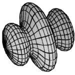
Figure 1: $\mathbb{CP}^{1}$ with metric induced from $G=(1,300,300,300,1).$

Now, in figure 2 we plot the evolution of the metric $G$ under the iterations of $T,T_{K}$, and $T_{\nu},$ respectively.

$r=0$ $r=1$ $r=2$ $r=3$ $r=4$

$T$:

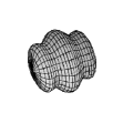
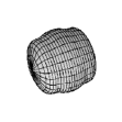
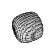
$T_{K}$:

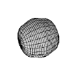
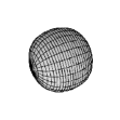
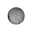
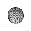
$T_{\nu}$:

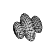
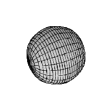
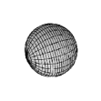
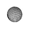
Figure 2: The first four iterations.

Clearly the $T$ iterations are much slower in converging to a round sphere. Not until the 3rd iteration does it become convex. At the other extreme lie the $T_{\nu}$ iterations where the first iteration is already almost indistinguishable from a round sphere. Intermediate between the two are the $T_{K}$ iterations. This visually depicts the the observations in section 3.2, where rates of convergence were compared using asymptotic behavior.

5 Higher dimensional projective space

Let us now investigate the complex projective space $X=\mathbb{CP}^{n}$ where $n>1$. We will consider exclusively the $T_{\nu}$ iteration. Let $z_{1},\ldots,z_{n}$ be local coordinates on $X=\mathbb{CP}^{n}$. Let us fix once and for all a volume form $\nu$ on $X$ by using that induced by the normalized Fubini-Study metric. That is if

$$\omega=\frac{\sqrt{-1}}{2\pi}\ \partial\overline{\partial}\,\log\left(1+\sum|z_{k}|^{2}\right)\phantom{XXXXX}$$

$$\phantom{XXXXX}=\frac{\sqrt{-1}}{2\pi}\ \frac{\sum_{i,j}\left[\left(1+\sum_{k}|z_{k}|^{2}\right)\delta_{ij}-z_{j}\overline{z}_{i}\right]}{\left(1+\sum_{k}|z_{k}|^{2}\right)^{2}}dz_{i}\wedge d\overline{z}_{j}$$

is the normalized Fubini-Study metric in local coordinates then we set

$$\nu=\omega^{n}=\,n!\,\left(\frac{\sqrt{-1}}{2\pi}\right)^{n}\frac{dz_{1}\wedge d\overline{z}_{1}\wedge\cdots\wedge dz_{n}\wedge d\overline{z}_{n}}{\left(1+|z_{1}|^{2}+\ldots+|z_{n}|^{2}\right)^{n+1}}.$$

It is not hard to check that with this choice of volume form we get

$$\mathrm{Vol}(\mathbb{CP}^{n})=\int_{\mathbb{CP}^{n}}\!\!\!\nu=1.$$

Again we set $L=O(1)$ and fix a $k>0$. Note that a basis of $H^{0}(X,L^{k})$ is given by the set of monomials in the $z_{i}$ of total degree $\leq k$. Denote these by $w_{1},\ldots,w_{N}$ where $N={n+k\choose k}$. In this set-up we are studying embeddings

$$X=\mathbb{CP}^{n}\hookrightarrow\mathbb{P}\left(H^{0}(\mathbb{CP}^{n},O(k))\right)\cong\mathbb{CP}^{N-1}.$$

As above we take $h$ to be the metric on $L^{k}=O(k)$ defined by

$$h=\left(\sum_{i=1}^{N}|w_{i}|^{2}\right)^{-1}.$$

Now if $G$ is a (positive definite Hermitian) matrix on $H^{0}(X,L^{k})$ then $T_{\nu}(G)$ is the matrix giving rise to the norm

$$\|s\|_{\mathrm{Hilb}_{\nu}}=R_{\nu}\int_{X}|s|_{h}^{2}\nu,$$

where

$$R_{\nu}=\frac{\mathrm{dim}\,H^{0}(X,L^{k})}{\mathrm{Vol}(X,\nu)}=N.$$

The matrix $G$ has rows and columns indexed by the terms $w_{i},\ i=1,\ldots,N$. Let us take a diagonal matrix with terms $a_{i}^{-1}$. Such a matrix corresponds to an (algebraic) metric invariant under the torus $\Lambda_{n}=(S^{1})^{n}$ action $z_{l}\mapsto e^{i\theta_{l}}z_{l},\ l=1,\ldots,n$.

An orthonormal basis, according to $G$, is given by

$$\left\{\sqrt{a_{i}}\,w_{i},i=1,\ldots,N\right\}.$$

Then in terms of the $a_{i}$’s the matrix $T_{\nu}(G)$ will have diagonal entries $\tilde{a}_{i}^{-1}$ equal to

$$\|w_{i}\|_{\mathrm{Hilb}_{\nu}}=Nn!\left(\frac{\sqrt{-1}}{2\pi}\right)^{n}\int_{\mathbb{C}^{n}}\frac{|w_{i}|^{2}dz_{1}\wedge d\overline{z}_{1}\wedge\cdots\wedge dz\wedge d\overline{z}_{n}}{\left(\sum_{p=1}^{N}a_{p}|w_{p}|^{2}\right)\left(1+\sum_{q=1}^{n}|z_{q}|^{2}\right)^{n+1}}.$$

Changing to polar coordinates $z_{j}=r_{j}\exp\left(\sqrt{-1}\ \theta_{j}\right)$ and substituting $x_{j}=r_{j}^{2}$ we get

$$T(G)_{ii}=\tilde{a}_{i}^{-1}=Nn!\int_{0}^{\infty}\cdots\!\!\int_{0}^{\infty}\frac{w_{i}(x)dx_{1}\cdots dx_{n}}{\left(\sum_{p=1}^{N}a_{p}w_{p}(x)\right)\left(1+\sum_{q=1}^{n}x_{q}\right)^{n+1}}$$ (12)

where $w(x)$ denotes the monomial $w$ with the substitutions $x_{k}=z_{k},k=1,\ldots,n$.

5.1 Asymptotic behavior in higher dimensions

Let us consider the asymptotic behavior of $T_{\nu}$. Recall (see section 3.2) that in the case of $n=1$, i.e. when $X=\mathbb{CP}^{1}$, we defined

$$\sigma_{T_{\nu},k}:=\lim_{r\rightarrow\infty}\frac{\mathrm{dist}(T_{\nu}^{(r+1)}(G),\ T_{\nu}^{(\infty)}(G))}{\mathrm{dist}(T_{\nu}^{(r)}(G),\ T_{\nu}^{(\infty)}(G))}.$$

This value depends on whether or not the initial metric $G$ is invariant under the inversion map $z\mapsto z^{-1}$, or equivalently in homogeneous coordinates $Z_{0}\leftrightarrow Z_{1}$. In [Don05b] Donaldson computes these values theoretically, and our investigations corroborate his result:

$$\sigma_{T_{\nu},k}=\left\{\begin{array}[]{rl}\frac{(k-1)k}{(k+2)(k+3)}&\mathrm{if\ }G\mathrm{\ is\ inv.\ under\ }Z_{0}\leftrightarrow Z_{1}\\ \frac{k}{(k+2)}&\mathrm{otherwise}\end{array}\right..$$ (13)

Our goal is to show evidence for a simple extension of this formula valid on $X=\mathbb{CP}^{n},\ n\geq 1$.

When $n>1$ there are many possible ways to extend the notion of a “palindromic” metric (as we defined in section 2): for the Riemann sphere we have those metrics invariant under $Z_{0}\leftrightarrow Z_{1}$ but in general there are many permutations of the homogeneous coordinates $Z_{0},\ldots,Z_{n}$ and it is trivial to check that if $G$ is a metric invariant under such a symmetry then so is $T_{\nu}(G)$. We might then expect that there can be distinct values for $\sigma$ depending on various symmetries the metric $G$ could be invariant under. Thus we may find a different value for each (conjugacy class of) subgroup of $\mathrm{Sym}(n+1)$ – the symmetric group on $n+1$ characters – corresponding to metrics $G$ invariant under the automorphisms $Z_{i}\mapsto Z_{\pi(i)},\ i=0,1,\ldots,n$ for $\pi$ ranging in the subgroup.

We present here some numerical findings in the cases of $n=2$ and $n=3$. The itereated integrals (equation 12) grow in computational complexity quickly with increasing $n$.

We start with a metric $G$ which is torus-invariant, but otherwise ‘random’ in the sense that it is not invariant under any permutation of the homogeneous coordinates. We tabulate approximate numerical values for the asymptotic constant $\sigma$ here, all computed starting with ‘random’ (but torus-invariant) metrics:

$\sigma$	$k=2$	3	4	5
$n=2$	0.40	0.50	0.57	0.63
3	0.33	0.43	0.50	0.56

For the moment let us just note that the above values apparently follow the pattern:

$$\sigma=\frac{k}{k+n+1}.$$ (14)

When $n=1$, the fundamental case which we considered, this formula specializes to (13).

The non-generic case, when $G$ might be invariant under a permutation of the homogeneous coordinate variables we find simple behavior:

• If there is no fixed-point-free permutation of the homogeneous coordinate variables under which $G$ is invariant then $\sigma$ is the same as computed in the asymmetric case.

• Otherwise suppose $G$ is invariant under some fixed-point-free permutation of the homogeneous coordinate variables. Then we get new values for $\sigma$, as tabulated in the following table:

$\sigma$	$k=2$	3	4	5
$n=2$	0.07	0.14	0.21	0.28
3	0.05	0.11	0.17	0.22

One can check that approximate fractional equivalents to these numbers follow the pattern

$$\sigma=\frac{(k-1)k}{(k+n+2)(k+n+3)}.$$ (15)

We should stress that when $n=1$ equation (15), together with (14), specializes to (13). This together with various experimental evidence leads the author to ask the following:

Question 5.1.

Let $G$ be a torus-invariant metric arising from a matrix on $H^{0}(\mathbb{CP}^{n},O_{\mathbb{CP}^{n}}(k))$, and let $B=T_{\nu}^{\infty}(G)$ be the limiting balanced metric under the $T_{\nu}$ iteration. Define

$$\sigma_{G}(n,k):=\lim_{r\rightarrow\infty}\frac{\mathrm{dist}(T_{\nu}^{(r+1)}(G),\ B)}{\mathrm{dist}(T_{\nu}^{(r)}(G),\ B)}.$$

Let us say that $G$ is generally symmetric if it is invariant under some fixed-point-free permutation of the homogeneous coordinates. Then do we have the general formula

$$\sigma_{G}(n,k)=\left\{\begin{array}[]{cl}\frac{(k-1)k}{(k+n+1)(k+n+2)}&\mathrm{if\ }G\mathrm{\ is\ generally\ symmetric}\\ \frac{k}{(k+2)}&\mathrm{otherwise}\end{array}\right.\quad?$$ (16)

5.2 Example computation

To illustrate a typical computation leading to some of the numbers above, take $n=3,k=4$. Then

$$N=\dim H^{0}\left(\mathbb{CP}^{3},O(4)\right)={3+4\choose 4}=35$$

and a basis of $H^{0}(\mathbb{CP}^{3},O(4))$ is (in local coordinates)

$$\{w_{1},\ldots,w_{35}\}=\{1,z_{1},z_{2},z_{3},z_{1}^{2},\ldots,z_{2}z_{3}^{3},z_{3}^{4}\}.$$ (17)

We choose a $G$ which is invariant under every permutation of the homogeneous coordinates $Z_{i},\,i=0,\ldots,3$ (where $z_{i}=\frac{Z_{i}}{Z_{0}}$). Taking into account these symmetries there are only five distinct basis elements:

$$1,\ z_{1},\ z_{1}^{2},\ z_{1}z_{2},\ z_{1}z_{2}z_{3}.$$

In the order the basis elements are listed in (17) – first by degree then lexicographically – these are the 1st, 2nd, 5th, 6th, and 15th elements. In the notation used at the beginning of this section we pick diagonal entries of $G$: $a_{i}^{-1}$ in the row and column determined by the basis element $w_{i}$. Due to the symmetries we will have five parameters:

$$G:a_{1},a_{2},a_{5},a_{6},a_{15}$$

The iterations of $T_{\nu}$ on these parameters – denote them by $a_{i,r},r=0,1,\ldots,\infty$ – will (after uniform scaling) tend toward the values $1,4,6,12,24$ for $i=1,2,5,6,15$ respectively. This can readily be checked by noting the Fubini-Study metric is the balanced metric $B$. At this point we should recall that the $a_{i}$ coefficients are actually entries in the inverse matrix $G^{-1}$, hence the entries of $G$ will tend to $1,1/4,1/6,1/12,1/24$. However it we can compute the approximate $\sigma$ values via

$$\lim_{r\rightarrow\infty}\frac{\mathrm{dist}(T_{\nu}^{(r+1)}(G),\ B)}{\mathrm{dist}(T_{\nu}^{(r)}(G),\ B)}.=\lim_{r\rightarrow\infty}\frac{\frac{1}{a_{2,r+1}}-\frac{1}{4}}{\frac{1}{a_{2,r}}-\frac{1}{4}}=\lim_{r\rightarrow\infty}\frac{a_{2,r+1}-4}{a_{2,r}-4}$$

say (note the last equality follows since the $a_{i},r$ are convergent). Denote this last quotient, within the limit, as $\tilde{\sigma}_{r+1}$. Its value should tend to the $\sigma$ value determining the asymptotic behavior of the $T_{\nu}$ iterations on this metric.

Let us take $(a_{1},a_{2},a_{5},a_{6},a_{15})=(1,20,30,40,50)$. The limiting balanced metric will have corresponding coordinates proportional to $(1,4,6,12,24)$ as noted above. However instead of uniformly scaling all metrics so the result is exactly this metric we will this time scale each metric so that its first coordinate (the $a_{1}$) is equal to one. There is no loss of information: relation (5) at the end of section (2) has the obvious adaptation to this situation; namely $\sum_{i=1}^{35}a_{i}/\tilde{a}_{i}=35$. Using this one can iteratively obtain the original numbers. The advantage of doing this is that we no longer need to keep track of the first coordinate $a_{1}$.

With this convention we get the following table for the first eight iterations, as well as the approximate $\sigma$ values:

$$\begin{array}[]{c|cccc|c}T_{\nu}^{(r)}&a_{2}&a_{5}&a_{6}&a_{15}&\tilde{\sigma}_{r}\\ \hline\cr 0&20.0000000&30.0000000&40.0000000&50.0000000&0.0000\\ 1&4.3071170&6.5967335&13.0915039&25.9850356&0.0192\\ 2&4.0344368&6.0688663&12.1588436&24.3600437&0.1121\\ 3&4.0052604&6.0105224&12.0258597&24.0613530&0.1528\\ 4&4.0008611&6.0017223&12.0042908&24.0102741&0.1637\\ 5&4.0001430&6.0002860&12.0007145&24.0017140&0.1661\\ 6&4.0000238&6.0000476&12.0001191&24.0002857&0.1665\\ 7&4.0000040&6.0000079&12.0000198&24.0000476&0.1666\\ 8&4.0000007&6.0000013&12.0000033&24.0000079&0.1667\par\par\end{array}$$

We note that the apparent limiting value, $0.1\overline{6}=1/6$, matches the value in equation (16).

6 Further Questions

The case of a non-diagonal matrix (thus corresponding to a metric not invariant under $z\mapsto e^{i\theta}z$) was not treated in this paper. Investigating this direction one might see whether the asymptotic values (see equations 9 and 10 in section 3.2, or 16 in section 5.2) remain valid, and whether the bound (11) given in section 3.3 still holds. If the bound does still hold then it would be interesting to work towards a sharp bound.

In another direction one might ask whether or not the operators $T,T_{\nu},T_{K}$ are distance decreasing after the first iteration; or put another way: is the square of each of these operators distance reducing? No counter example to this was found.

The next step is to look beyond $\mathbb{CP}^{n}$, perhaps to toric varieties (see for example [BD08]), $K3$ surfaces, Calabi-Yau $3$-folds, etc., and work out the same convergence properties of these dynamical systems. It would also be interesting to compare the convergence properties of the $T$-iterations to those of PDE methods for finding canonical metrics, such as the Ricci flow. All these questions the author hopes to examine later.

References

[BD08]
R. S. Bunch and S. K. Donaldson.
Numerical approximations to extremal metrics on toric surfaces.
arXiv:0803.0987v1, 2008.
[CC02]
E. Calabi and X. Chen.
The space of Kähler metrics (ii).
J. Differential Geom., 61:173–193, 2002.
[Che00]
X. Chen.
The space of Kähler metrics.
J. Differential Geom., 56(2):189–234, 2000.
[DKLR06a]
M. Douglas, R. Karp, S. Lukic, and R. Reinbacher.
Numerical Calabi-Yau metrics.
arXiv:hep-th/0612075, 2006.
[DKLR06b]
M. Douglas, R. Karp, S. Lukic, and R. Reinbacher.
Numerical solution to the Hermitian Yang-Mills equation on the
Fermat quintic.
arXiv:hep-th/0606261, 2006.
[Don99]
S. K. Donaldson.
Symmetric spaces, Kähler geometry and Hamiltonian dynamics.
In Northern California Symplectic Geometry Seminar, volume 196
of Amer. Math. Soc. Transl. Ser. 2, pages 13–33. Amer. Math. Soc.,
Providence, RI, 1999.
[Don01]
S. K. Donaldson.
Scalar curvature and projective embeddings. I.
J. Differential Geom., 59(3):479–522, 2001.
[Don02]
S. K. Donaldson.
Scalar curvature and stability of toric varieties.
J. Differential Geom., 62(2):289–349, 2002.
[Don05a]
S. K. Donaldson.
Scalar curvature and projective embeddings. II.
Q. J. Math., 56(3):345–356, 2005.
[Don05b]
S. K. Donaldson.
Some numerical results in complex differenital geometry.
arXiv:math/0512625v1 [math.DG], 2005.
[HW06]
M. Headrick and T. Wiseman.
Numerical Ricci-flat metrics on K3.
arXiv:hep-th/0506129, 2006.
[Kel07a]
J. Keller.
Ricci iteration on Kähler classes.
arXiv:0709.1490v2, 2007.
[Kel07b]
J. Keller.
Web page.
http://www.ma.ic.ac.uk/~jkeller/Julien-KELLER.html, 2007.
[Luo98]
H. Luo.
Geometric criterion for Gieseker-Mumford stability of polarized
manifolds.
J. Differential Geom., 49(3):577–599, 1998.
[Mab87]
T. Mabuchi.
Some symplectic geometry on compact Kähler manifolds. I.
Osaka J. Math., 24(2):227–252, 1987.
[Mab05]
T. Mabuchi.
An energy-theoretic approach to the Hitchin-Kobayashi
correspondence for manifolds. I.
Invent. Math., 159(2):225–243, 2005.
[PS03]
D. H. Phong and J. Sturm.
Stability, energy functionals, and Kähler-Einstein metrics.
Comm. Anal. Geom., 11(3):565–597, 2003.
[PS06]
D. H. Phong and J. Sturm.
The Monge-Ampère operator and geodesics in the space of
Kähler potentials.
Invent. Math., 166(1):125–149, 2006.
[Rub07]
Y. Rubinstein.
Some discretizations of geometric evolution equations and the Ricci
iteration on the space of Kähler metrics.
arXiv:0709.0990v1, 2007.
[San06]
Y. Sano.
Numerical algorithm for finding balanced metrics.
Osaka J. Math., 43(3):679–688, 2006.
[Sem92]
S. Semmes.
Complex Monge-Ampère and symplectic manifolds.
Amer. J. Math., 114(3):495–550, 1992.
[Tia90]
G. Tian.
On a set of polarized Kähler metrics on algebraic manifolds.
J. Differential Geom., 32(1):99–130, 1990.
[Tia97]
G. Tian.
Kähler-Einstein metrics with positive scalar curvature.
Invent. Math., 130(1):1–37, 1997.
[Yau78]
S.-T. Yau.
On the Ricci curvature of a compact Kähler manifold and the
complex Monge-Ampère equation. I.
Comm. Pure Appl. Math., 31(3):339–411, 1978.
[Yau93]
S.-T. Yau.
Open problems in geometry.
In Differential geometry: partial differential equations on
manifolds (Los Angeles, CA, 1990), volume 54 of Proc. Sympos. Pure
Math., pages 1–28. Amer. Math. Soc., Providence, RI, 1993.
[Zha96]
S. Zhang.
Heights and reductions of semi-stable varieties.
Compositio Math., 104(1):77–105, 1996.