Boltzmann equation for dissipative gases in homogeneous states with nonlinear friction

Abstract

Combining analytical and numerical methods, we study within the framework of the homogeneous non-linear Boltzmann equation, a broad class of models relevant for the dynamics of dissipative fluids, including granular gases. We use the new method presented in a previous paper [J. Stat. Phys. 124, 549 (2006)] and extend our results to a different heating mechanism, namely a deterministic non-linear friction force. We derive analytically the high energy tail of the velocity distribution and compare the theoretical predictions with high precision numerical simulations. Stretched exponential forms are obtained when the non-equilibrium steady state is stable. We derive sub-leading corrections and emphasize their relevance. In marginal stability cases, power-law behaviors arise, with exponents obtained as the roots of transcendental equations. We also consider some simple BGK (Bhatnagar, Gross, Krook) models, driven by similar heating devices, to test the robustness of our predictions.

I Introduction

Granular materials represent one of the most well-known paradigms for open dissipative systems; their ubiquitous character in natural phenomena or industrial processes, the possibility to study them at both very applied and very fundamental levels have prompted many efforts to understand their properties Jaeger ; PoschelBrill ; barrat05 ; poschel01 ; poschel03 , but they remain challenging from many points of view. Thermodynamic-like descriptions remain in particular elusive for these intrinsically far from equilibrium systems, because energy is continuously lost through internal dissipation, and has to be compensated by non-thermal sources.

Dilute granular gases present a particularly interesting framework which can be studied by model experiments, numerical simulations, hydrodynamics, kinetic theory or more phenomenological approaches. The investigation of the velocity distribution of the particles reveals a rich phenomenology, with strong deviations from the equilibrium Maxwell-Boltzmann behavior, and its description is still an object of debates. From an experimental point of view, the situation may appear confusing at first sight. Although the measured velocity distribution $F({\bf v})$ generically deviates from the Maxwellian, its functional form depends on material property and on the forcing mechanism used to compensate for collisional loss of energy Exp ; Prevost ; EPJE ; Aranson . A similar picture emerges from numerical simulations and analytical studies Aranson ; Gold ; Brey ; puglisi ; Rome ; Fuchs ; stretch-tails ; MS ; Cafiero ; Swinney ; Santos ; Maxwell ; KBN02 ; EB-JSP ; EB-PRE ; Math ; BBRTvW ; Pias ; ben-Avb ; EPJE ; Zip ; vanZon ; Haifa ; EBN-Machta ; JSP-1 ; EPL , where in addition to the more common stretched exponential behavior, power-law distributions have also been reported Rome ; Maxwell ; KBN02 ; EB-JSP ; EBN-Machta .

Since the universality of the Maxwell-Boltzmann distribution for equilibrium gases seems to have no analog in steady states of dissipative gases, it is necessary to identify the generic trends for the velocity distribution and study their properties in a unified and simple framework. Our purpose is to develop further an existing quantitative cartoon to unveil the different effects at work, that lead to the wide range of behaviors alluded to above, when certain key parameters are changed. To this aim, we focus on the framework of the generalized inelastic Boltzmann equation, which describes dilute homogeneous dissipative gases. The study of homogeneous systems is not only a useful starting point, it is also relevant to experiments with bulk driving Prevost ; Aranson . Spatial heterogeneity (and thus gravity, hydrodynamic instabilities, shock formation and clustering PoschelBrill ) will henceforth be discarded.

The most characteristic features of the velocity distribution in dissipative systems – whether observed in time dependent scaling states or in non-equilibrium steady states – is overpopulated high energy tails. Generically these tails are stretched exponentials stretch-tails ; MS ; EB-PRE . The more spectacular power law tails Rome ; Maxwell ; KBN02 ; EB-JSP ; EBN-Machta are exceptional. They were only found in systems of Maxwell molecules, and in the unusual device of Ref.EBN-Machta . In general these power law tails do not evolve naturally, but require careful fine-tuning of the physical parameters, both in the interactions, and in the driving mechanisms JSP-1 ; EPL .

In the present paper, specific features and properties of $F(v)$ will be derived and analyzed, when energy is injected by a negative friction thermostat, parametrized by an exponent $\theta$. An important new result of general importance EPL ; JSP-1 is also the direct and simple relation between the parameters controlling the stability of the energy balance equation, i.e. the balance between collisional dissipation and energy injection on the one hand, and on the other hand the occurrence of new power law tails $\sim 1/v^{a(\theta)}$ in the velocity distribution of the non equilibrium steady state, which appear at the margin of stability in this equation. In Ref. EPL a short summary of our results was presented. In this longer paper we show how all these results, and in particular these new power law tails, have been obtained with the help of a new method developed in Ref.EPL ; JSP-1 , which is applicable to different types of forcing mechanisms, and to a large class of interaction models, including inelastic hard spheres and Maxwell molecules. It seems virtually impossible to obtain the present results by using the old methods developed for Maxwell molecules Rome ; Maxwell ; EB-JSP .

The current paper hence constitutes a sequel to our first study JSP-1 , in which we have developed a method for analyzing the deviations of $F(\bf v)$ from Gaussian behavior. While we have focused in JSP-1 on granular gases for which energy is injected by random forces, we consider here a different driving mechanism. We show that the large velocity tail of $F({\bf v})$ is characterized by a stretched exponential $\exp[-v^{b}]$ with an exponent $b$, that governs the stability of the non-equilibrium steady state. When this state is a stable fixed point of the dynamics, the exponent satisfies $b>0$. For the exceptional cases of marginal stability, where $b$ vanishes, $F$ is of power law type, and the corresponding exponents will be calculated.

The paper is organized as follows: we recall in section II the Boltzmann equation for inelastic soft spheres, together with the criterion of stability of non-equilibrium steady states (NESS). We also briefly recall in II.2 the method introduced in our previous paper JSP-1 . Sections III and IV give the results for the large velocity tail of the velocity distribution in the case of energy injection by non-linear negative friction, for both stable and marginally stable NESS. We turn in section V to a simple linear model which mimics the basics of the inelastic Boltzmann equation. While this BGK model is amenable to analytical treatment, we show that it does not reproduce the rich behavior of the non-linear Boltzmann equation, in particular it fails for hard interactions. Section VI finally contains our conclusions.

II Inelastic Boltzmann equation

We consider the Boltzmann equation for a gas of inelastic soft spheres JSP-1 , which represents one of the simplest models for rapid granular flows. The dynamics is described as a succession of uncorrelated inelastic binary collisions, modelled by soft spheres with a collision frequency and a coefficient of normal restitution $\alpha$, where $0<\alpha<1$ PoschelBrill . The collision law $({\bf v}_{1},{\bf v}_{2})\to({\bf v}^{\prime}_{1},\bf v^{\prime}_{2})$ reads:

$${\bf v}^{\prime}_{1}={\bf v}_{1}-p({\bf{g}}\!\cdot\!{\bf{n}}){\bf{n}},\quad{{\bf v}^{\prime}_{2}}={{\bf v}_{2}}+{p}({\bf{g}}\!\cdot\!{\bf{n}})\bf{n}$$ (1)

where $\bf{g}\equiv{\bf v}_{1}-{\bf v}_{2}$, $p=1-q=\frac{1}{2}(1+\alpha)$ and $\bf{n}$ is a unit vector parallel to the impact direction connecting particles 1 and 2. Inelastic collisions conserve mass and momentum, and dissipate kinetic energy at a rate $\propto{1\over 2}(1-\alpha^{2})=2pq$ (the elastic case corresponds to $\alpha=1$). We consider a general collision frequency, $g\varsigma(g,\vartheta)\sim g^{\nu}|\widehat{\bm{g}}\cdot\bf{n}|^{\sigma}$. Here $\varsigma(g,\vartheta)$ is the differential scattering cross section with $\vartheta=\cos^{-1}(\widehat{\bm{g}}\cdot\bf{n})$, $\nu$ describes its energy dependence, and $\sigma$ its angular dependence. The exponent $\sigma\neq 1$ describes a distribution of impact parameters biased towards grazing ($\sigma<1$) or head-on ($\sigma>1$) collisions. For mathematical convenience models with $\sigma=\nu$ have also been considered KBN02 ; EB-JSP ; JSP-1 . The symbol $\mathbf{\widehat{a}}={\bf a}/a$ denotes a unit vector, parallel to $\bf{a}$. For elastic particles interacting via a soft sphere potential $U(r)\propto r^{-a}$, one has $\nu=1-2(d-1)/a$ Phys-Rep-ME , where $d$ is the space dimension. The exponents $\nu=\sigma=1$ correspond to standard hard-sphere behavior $(a\to\infty)$, while $\nu=0$ corresponds to Maxwell molecules ($a=2(d-1)$). Here $\nu$ and $\sigma$ will be free exponents, that parametrize the material properties together with the inelasticity parameter $\alpha$.

We now give a simple representation of the nonlinear Boltzmann collision operator, which is convenient to study the spectral properties of the linearized collision operator. The time dependent distribution $F({\bf v},t)$ in spatially homogeneous systems obeys the nonlinear Boltzmann equation EPL :

$$\partial_{t}F({\bf v},t)+{\cal F}F=I(v|F)\equiv\int_{\bf n}\int d{\bf v}_{1}d{\bf v}_{2}g^{\nu}|\widehat{\bf{g}}\cdot\bf{n}|^{\sigma}\times$$

$$F({\bf v}_{1},t)F({\bf v}_{2},t)[\delta({\bf v}-{\bf v}^{\prime}_{1})-\delta({\bf v}-{\bf v}_{1})]$$ (2)

where the collision operator $I(v|F)$ has the usual gain-loss structure. For anisotropic $F({\bf v},t)$ the angular integral, $\int_{\bf n}(\cdots)=\int^{(-)}d{\bf n}(\cdots)/\int^{(-)}d{\bf n}$ denotes an average over the pre-collision hemisphere, $\mathbf{g}\cdot{\bf{n}}\leq 0$. For isotropic distributions, as considered here, the integrals over pre- and post-collision hemisphere are the same, and $\int_{\bf n}(\cdots)=\int d{\bf n}(\cdots)/\Omega_{d}$ can be extended over the complete solid angle, i.e. where $\Omega_{d}=2\pi^{d/2}/\Gamma(d/2)$ is the surface area of a $d$-dimensional unit sphere, and $\Gamma(x)$ is the Gamma function.

The forcing term ${\cal F}F$ represents the energy supply, working against inelastic dissipation. It may lead to a NESS (Non-Equilibrium Steady State). Absence of forcing ($\mathcal{F}=0$) describes free cooling, where the energy is decreasing in time. A heating device, considered frequently, consists in a random force acting on the particles in between collisions: the corresponding stochastic White Noise (WN), widely used in analytical and numerical studies stretch-tails ; Pago ; MS ; Swinney ; BBRTvW ; vanZon , is described by adding a diffusion term $-D{\bf\partial}_{\bf v}^{2}F$ to the Boltzmann equation. Our previous paper JSP-1 has focused on this case. An interesting alternative is given by deterministic nonlinear Negative Friction (NF). In general, the forcing term reads

$${\cal F}F=({\cal F}_{\rm NF}+{\cal F}_{\rm WN})F=\gamma\partial_{{\bf v}}\cdot({\bf v}v^{\theta-1}F)\,-\,D\,\partial_{{\bf v}}^{2}F$$ (3)

with ($\gamma=0$, $D\neq 0$) for WN and ($\gamma>0$, $D=0$) for NF, and $\theta\geq 0$. The value $\theta=1$ corresponding to the Gaussian thermostat allows us to study the long time scaling regime of an unforced system (so-called free cooling) (see section II.1 and MS ). The special case $\theta=0$ models gliding friction. In general $\theta$ is a continuous exponent selectively controlling the energy injection mechanism. In summary, the ’phase space’ to explore is thus given by the parameters ($\nu,\sigma,\theta,\alpha$) for NF driving, which is the main focus of this paper.

The explicit form of $I(v|F)$ above is convenient for calculating the rate of change of averages, $\int{d{\bf v}}\psi(v)F(v,t)\equiv\langle\psi|F\rangle_{t}$, i.e.

$$\partial_{t}\>\langle\psi({\bf v})|F\rangle_{t}+\langle\psi|{\cal F}F\rangle_{t}= \frac{1}{2} \int_{\bf n}\int d{\bf v}_{1}d{\bf v}_{2}\>g^{\nu}|\widehat{\bf{g}}\cdot\bf{n}|^{\sigma}\times$$

$$F({\bf v}_{1},t)F({\bf v}_{2},t)[\psi({\bf v}^{\prime}_{1})+\psi(\! \!{\bf v}^{\prime}_{2}\! \!)-\psi({\bf v}_{1})-\psi({\bf v}_{2})]$$ (4)

Here II is just a special case of II, where $\langle\psi({\bf v})|F\rangle_{t}=F({\bf w},t)$ for $\psi({\bf v})=\delta({\bf v}-{\bf w})$. The loss rate of energy follows by setting $\langle\psi({\bf v})|F\rangle_{t}=\langle\frac{1}{2}mv^{2}|F\rangle_{t}\equiv\frac{d}{4}mv_{0}^{2}(t)$, where $v_{0}(t)$ is the r.m.s. velocity and $v^{2}_{0}$ the granular temperature. We further use the normalizations, $\langle(1,{\bf v},v^{2})|F\rangle_{t}=(1,0,dv_{0}^{2}(t)/2)$.

II.1 Scaling form and stability of steady states

To analyze the behavior of the distribution function we assume a rapid approach to a scaling form,

$$F(v,t)=(1/v_{0}(t))^{d}f(v/v_{0}(t))$$ (5)

(for related proofs, see Math ) with normalizations

$$\langle(1,c^{2})|f\rangle=(1,d/2).$$ (6)

The inelastic Boltzmann equation II can then be decoupled into a time-independent equation for the scaling form $f(c)$ and a time-dependent equation for the r.m.s. velocity $v_{0}$, or granular temperature $v^{2}_{0}$, which reads

$$\frac{d}{dt}\left(\frac{d}{2}v^{2}_{0}\right)=\langle v^{2}|I\rangle_{t}-\langle v^{2}|\mathcal{F}F\rangle_{t}.$$ (7)

The collisional average $\langle v^{2}|I\rangle_{t}$ follows from II and 1 by carrying out the angular average, and by inserting 5 to change to scaling variables. Here $\int_{\bf n}|\widehat{{\bf g}}\cdot{\bf n}|^{\sigma+2}=\beta_{\sigma+2}$ is given by

$$\beta_{\sigma}=\int_{\bf n}|\widehat{{\bf g}}\cdot{\bf n}|^{\sigma}=\textstyle{\Gamma(\frac{\sigma+1}{2})\Gamma(\frac{d}{2})/\Gamma(\frac{\sigma+d}{2})\Gamma(\frac{1}{2})}$$ (8)

where $\beta_{\sigma}$ is well defined for $\sigma>-1$. The forcing terms, $\langle v^{2}|\mathcal{F}F\rangle_{t}$ are calculated along the same lines using 3 and partial integrations. The results are,

$$\langle v^{2}|I\rangle_{t}=-\textstyle{\frac{1}{2}}\lambda_{2}\langle\langle g^{\nu+2}\rangle\rangle v_{0}^{\nu+2}(t)$$

$$\langle v^{2}|\mathcal{F}_{\rm WN}F\rangle_{t}=-2dD$$

$$\langle v^{2}|\mathcal{F}_{\rm NF}F\rangle_{t}=-2\gamma\langle c^{\theta+1}\rangle v_{0}^{\theta+1}(t),$$ (9)

where $g=|{\bf c}_{1}-{\bf c}_{2}|$. The coefficient $\lambda_{2}=2pq\beta_{\sigma+2}$ can be identified as the eigenvalue of the linearized Boltzmann collision operator (see the general expression for $\lambda_{s}$ below, Eq. (18) next subsection). Here, the notation $\langle\langle k({\bf c}_{1},{\bf c}_{2})\rangle\rangle$ stands for the average of a function $k({\bf c}_{1},{\bf c}_{2})$ with weight $f({\bf c}_{1})f({\bf c}_{2})$.

Let us first consider forced systems. The two terms in (7) can then balance each other and lead to a NESS. For the WN-driven case ($\gamma=0$), Eqs.7-II.1 give

$$dv^{2}_{0}/dt = 4D-\textstyle{\frac{1}{d}}\lambda_{2}\langle\langle g^{\nu+2}\rangle\rangle v_{0}^{\nu+2}(t)$$ (10)

$$= 4D\left[1-\left(\textstyle{\frac{v_{0}(t)}{v_{0}(\infty)}}\right)^{2b}\right]$$

where $b_{\rm WN}=1+\textstyle{\frac{1}{2}}\nu$, and $v_{0}(\infty)$ is defined as the stationary solution of 10. Similarly we obtain for the NF-case,

$$dv_{0}/dt = (\textstyle{\frac{2\gamma}{d}})\langle c^{\theta+1}\rangle v_{0}^{\theta}(t)-\textstyle{\frac{\lambda_{2}}{2d}}\langle\langle g^{\nu+2}\rangle\rangle v_{0}^{\nu+1}(t)$$ (11)

$$= (\textstyle{\frac{2\gamma}{d}})\langle c^{\theta+1}\rangle v_{0}^{\theta}(t)\left[1-\left(\frac{v_{0}(t)}{v_{0}(\infty)}\right)^{b}\right]$$

where $b_{\rm NF}=\nu+1-\theta$. The dynamics always admits a fixed point solution of the equations above. The fixed point solution $v_{0}(\infty)$ is stable/attracting for $b>0$, unstable/repelling for $b<0$, and marginally stable for $b=0$. As long as $b>0$, the system naturally evolves towards the stable NESS. Note that $D$ and $\gamma$ in 10 and 11 are irrelevant phenomenological constants, that can be absorbed in energy and time scales.

In the stable NESS $(\dot{v}_{0}=0,b>0)$, the corresponding integral equations for $f(c)$ follow from II with $\partial_{t}F=0$ and 3, and yield respectively for WN and NF,

$$I(c|f)=-\frac{D}{(v_{0}(\infty))^{2b}}\partial^{2}_{{\bf c}}f=-\frac{\lambda_{2}}{4d}\langle\langle g^{\nu+2}\rangle\rangle\partial^{2}_{{\bf c}}f$$ (12)

$$I(c|f)=\frac{\gamma}{(v_{0}(\infty))^{b}}\partial_{{\bf c}}\!\cdot\!(\widehat{{\bf c}}c^{\theta}f)=\frac{\lambda_{2}\langle\langle g^{\nu+2}\rangle\rangle}{4\langle c^{\theta+1}\rangle}{\partial}_{{\bf c}}\!\cdot\!(\widehat{{\bf c}}c^{\theta}f)$$ (13)

Here $D$ and $\gamma$ have been eliminated with the help of the steady state solutions of 10 and 11.

It is also possible to consider the freely evolving state (FC), that does not lead to a NESS since $\gamma=0$ and $D=0$, but to a scaling solution $f(c)$. Here the r.m.s. velocity decays according to

$$\dot{v}_{0}=-\textstyle{\frac{\lambda_{2}}{2d}}\langle\langle g^{\nu+2}\rangle\rangle v_{0}^{\nu+1}(t).$$ (14)

Moreover comparison of the FC case with the Gaussian thermostat (NF: $\theta=1$) shows that the corresponding integral equations for $f(c)$ are identical, as observed in MS . This occurs because the term arising from $\partial_{t}F$ in II for FC is non-zero (since we do not have a NESS) and corresponds exactly with the forcing term in Eq. 13 when $\theta=1$ (since $\langle c^{2}\rangle=d/2$). The Gaussian thermostat in fact describes a system driven by a linear (negative) friction force, ${\bf a}=\gamma{\bf c}$. This corresponds to a linear rescaling of the velocities, which leaves $f(c)$ invariant. While the NF with $theta=1$ and FC states are equivalent at the level of the scaled velocity distribution function, they differ in the evolution equation for the temperature. It is therefore not possible to extend the stability criterion of NF to FC systems.

We also note that 14 gives a generalization of Haff’s law, that describes the decay of the energy or granular temperature for inelastic soft spheres. For instance, for $\nu>0$ one finds $v^{2}_{0}(t)\sim t^{-2/\nu}$ (for more details, see JSP-1 ).

II.2 Linearized Boltzmann operator

We now recall briefly the method introduced in JSP-1 , which allows us to obtain the behavior of the velocity distributions at large velocities. Suppose that for large $c=v/v_{0}$ the velocity distribution can be separated into two parts, $f(c)=f_{0}(c)+h(c)$, where $h(c)$ is the singular tail part that we want to determine, and $f_{0}(c)$ the presumably regular bulk part. The tail part $h(c)$ may be exponentially bound $\sim\exp[-\beta c^{b}]$ with $0<b<2$, or of power law type. In the bulk part $f_{0}(c)$ the variable $c$ is effectively restricted to bulk values in the thermal range $v\lesssim v_{0}$ or $c\lesssim 1$. As far as large velocities are concerned, the thermal range of $f$ may be viewed to zeroth approximation as a Dirac delta function $\delta({\bf c})$, carrying all the mass of the distribution. In this way, we obtain an asymptotic expansion of $f(c)$ by considering the ansatz

$$f(c)=\delta({\bf c})+h(c),$$ (15)

and linearizing the collision term $I(c|f)$ around the delta function (using the relation $I(c|\delta)=0$). This defines the linearized Boltzmann collision operator,

$$I(c|\delta+h)=-\Lambda h(c)+{\cal O}(h^{2}).$$ (16)

Note that we restrict the analysis to isotropic functions $h(c)$. The eigenfunctions of $\Lambda$ decay like powers $c^{-s}$. Consequently they are very suitable for describing power law tails, $f(c)\sim c^{-s}$. We note, however, that the moments $\int d{\bf c}c^{s}f(c)$ are largely determined by the regular bulk part, which can therefore not be approximated by $\delta({\bf c})$ when calculating moments.

The most important spectral properties are the eigenvalues and right and left eigenfunctions,

$$\Lambda c^{-s-d-\nu}=\lambda_{s}c^{-s-d}\quad;\quad\Lambda^{\dagger}c^{s}=\lambda_{s}c^{s+\nu}$$ (17)

with eigenvalues for $s>0$ JSP-1 ,

$$\lambda_{s}=\beta_{\sigma}\left\{1-_{2}\!F_{1}\,\left(\textstyle{-\frac{s}{2},\frac{\sigma+1}{2};\frac{\sigma+d}{2}}\,|\,1-q^{2}\right)\right\}-p^{s}\beta_{s+\sigma}.$$ (18)

Here ${}_{2}F_{1}(a,b;c|z)$ is a hyper-geometric function and $\beta_{\sigma}$ is given by (8). The value $s=0$ with $\lambda_{0}=0$ is an isolated point of the spectrum with corresponding stationary eigenfunctions, invariant under collisions,

$$\Lambda\delta({\bf c})=0\qquad\mbox{and}\qquad\Lambda^{\dagger}\cdot 1=0\qquad(\lambda_{0}=0).$$ (19)

Right and left eigenfunctions are different because $\Lambda$ is not self-adjoint. There is in fact among the eigenfunctions in 17 another, less trivial, stationary right eigenfunction, $c^{-s^{*}-d-\nu}$, where $s^{*}$ is the root of transcendental equation $\lambda_{s}=0$ (see JSP-1 ).

We also note that the eigenvalue $\lambda_{s}$ is independent of the energy exponent $\nu$: it is the same for inelastic Maxwell molecules, hard spheres, very hard particles, and very weakly interacting particles. The reason is presumably that the scattering laws are the same in all models, and equal to those of inelastic hard spheres. Moreover, it depends strongly on the inelasticity through $\alpha$, and weakly on the angular exponent $\sigma$. Fig. 1 shows that $\lambda_{s}$ is a concave function of $s$.

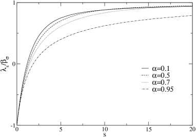
Figure 1: Concave eigenvalue spectrum $\lambda_{s}(\sigma)$ for $s\geq 0$ of the collision operator in the inelastic soft sphere models $\{\sigma,\nu\}$, defined in the text, and shown for various values of the coefficient of restitution $\alpha$. The ordinate shows $\lambda_{s}(\sigma)/\beta_{\sigma}$ for $d=2,\sigma=\nu=1$, which approaches 1 for $s\to\infty$, and -1 for $s\to 0$. The point $\lambda_{0}(\sigma)=0$ is an isolated point of the spectrum.

The previous paragraphs refer to the action of the $I(c|f)$ on functions $f(c)$ of power law type. We shall also need the large-$c$ form, $I_{\infty}$, of the collision operator acting on exponentially bound functions, $f(c)\sim\exp[-\beta c^{b}]$, with positive constants $\beta,b$. The nonlinear operator reduces to a linear one for $c_{1}\gg c_{2}$, because $\mathbf{g}\sim\mathbf{c}_{1}$ and $\mathbf{c}^{\prime}_{1}=\mathbf{c}-p(\mathbf{c}_{1}\cdot\mathbf{n})\mathbf{n}$, and the $\mathbf{c}_{2}$-integration can be carried out in II. The resulting expression is,

$$I_{\infty}(c|f)=-\beta_{\sigma}c^{\nu}[1-{\cal K}_{\sigma}c^{-b(\sigma+1)/2}]f(c),$$ (20)

and we obtain for the coefficient,

$${\cal K}_{\sigma}=\textstyle{\left({\Gamma(\frac{d+\sigma}{2})}/{\Gamma(\frac{d-1}{2})}\right)}\left(({2}/{\beta b(1-q^{2})})^{(\sigma+1)/2}\right)$$ (21)

as derived in Appendix B of Ref.JSP-1 . Note also that this coefficient vanishes in one dimension.

III Asymptotics for stable NESS

Exact closed forms of the scaling solution of 13 are not known in general, but the high energy tail may be computed accurately with the method developed in Ref. JSP-1 . Restricting the analysis to standard arguments where the asymptotic form of $I(c|f)$ is $I_{\infty}(c|f)\sim-\beta_{\sigma}c^{\nu}$ (see e.g. stretch-tails ), an interesting feature emerges JSP-1 ; EPL : in the region of stability ($b>0$), the asymptotic solution of 13 has a stretched exponential form, $f\sim\exp[-c^{b}]$, with $b=\nu+1-\theta$, while in cases of marginal stability ($b\to 0^{+}$), $f\sim c^{-a}$ is of power law type with an a priori unknown exponent $a$. As expected, $b$ decreases when $\nu$ decreases, since a tail particle with velocity $c\gg 1$ suffers collisions at a rate $c^{\nu}$. The slower the rate, the slower the particle redistributes its energy over the thermal range $c\lesssim 1$, which results in an increasingly overpopulated high energy tail. When $\nu$ is further decreased such that $b$ changes sign, the tail is no longer able to equilibrate with the thermal “bulk”, and the system cannot sustain a steady state. A similar intuitive picture may be developed with respect to $\theta$ in the NF cases EPL .

The leading behavior of $f(c)$ is a generalization of the one obtained for inelastic hard spheres ($\nu=1$) and Maxwell molecules ($\nu=0$). While we had analyzed in details the case of WN driving in JSP-1 , we focus here on inelastic gases driven by NF, which include the Gaussian thermostat, or equivalently, the Freely Cooling gas (FC: $\theta=1$). The method allows us to calculate the sub-leading correction for $c\gg 1$ to $I_{\infty}(c|f)$. This in turn yields important sub-leading multiplicative correction factors to $f(c)$ of exponential and power law type, i.e.

$$\ln f(c)\sim-\beta c^{b}+\beta^{\prime}c^{b^{\prime}}+\chi\ln c+\mathcal{O}(1),$$ (22)

where $b>b^{\prime}>0$. This expression is in fact an asymptotic expansion of $\ln f(c)$. The limiting corrections as $b^{\prime}\to 0^{+}$ are already contained in the exponent $\chi$. Moreover, as soon as $b^{\prime}$ becomes negative, the correction term becomes $c^{-|b^{\prime}|}\ll\mathcal{O}(1)$, and should be neglected for consistency. In the spirit of asymptotic expansions we only look for the sub-dominant correction $c^{b^{\prime}}$ with $b^{\prime}>0$ and set $\chi=0$. Only if $b^{\prime}=0$ do we look for terms of type $\chi\ln c$. The goal of this section is to calculate the exponents $\{b,b^{\prime},\chi\}$ explicitly, and to express the coefficients $\{\beta,\beta^{\prime}\}$ in terms of the moments $\langle\langle g^{\nu+2}\rangle\rangle$ and $\langle c^{\theta+1}\rangle$. These moments can be independently measured in the DSMC (Direct Simulation Monte Carlo) method (see Ref. JSP-1 ). The sub-leading approximation supposedly extends the agreement of theoretical predictions with measured DSMC data to smaller $c$-values.

We start with the NF integral equation, obtained from 13 by replacing the collision operator $I$ by the full asymptotic form $I_{\infty}$ in 20. The last form is the appropriate one for exponentially bound functions $f(c)$. This yields

$$-\mathcal{B}_{\sigma}c^{\nu}\{1-{\cal K}_{\sigma}(d)c^{-\textstyle{\frac{1}{2}}(\sigma+1)b}\}f=c^{\theta}f^{\prime}+(d+\theta-1)c^{\theta-1}f,$$ (23)

where the $c$-independent factors have been combined into,

$$\mathcal{B}_{\sigma}=\frac{4\beta_{\sigma}\langle c^{\theta+1}\rangle}{\lambda_{2}\langle\langle g^{\nu+2}\rangle\rangle}=\frac{2(d+\sigma)\langle c^{\theta+1}\rangle}{(1+\sigma)pq\langle\langle g^{\nu+2}\rangle\rangle},$$ (24)

and $\lambda_{2}=2pq\beta_{\sigma+2}$ and 8 have been used. Here the constant $\mathcal{B}_{\sigma}$ depends on all three model parameters $(\nu,\sigma,\theta)$, and contains averages with the unknown weight $f(c)$.

The parameters in $f(c)$ can be obtained from the full integral equation 23 by substituting the ansatz 22, applying the derivative, equating leading and sub-leading powers of $c$, and recalling the relation $b>b^{\prime}>0$. To leading order we have $b\beta c^{b+\theta-1}=c^{\nu}{\cal B}_{\sigma}$, yielding

$$b=\nu+1-\theta;\qquad\beta b=\mathcal{B}_{\sigma}.$$ (25)

The exponent $b$ is the same as the one found in the stability analysis in 11. These results are largely generalizations of special cases, existing in the literature for $\theta=\{0,1\};\nu=\{0,1\};\sigma=\{1,\nu\}$, derived in stretch-tails ; MS .

The remaining terms with sub-leading powers of $c$ have respectively the exponents $E_{1}=b^{\prime}+\theta-1,E_{2}=\theta-1,E_{3}=\nu-\textstyle{\frac{1}{2}}(\sigma+1)b$. First consider the case $\sigma=1$, where $E_{3}=\nu-b=\theta-1=E_{2}$. As $E_{1}>E_{2}$ the coefficient $\beta^{\prime}=0$, equating the coefficients of the remaining terms then yields the second line of the equation III below. If $\sigma>1$, then $E_{1}>E_{2}>E_{3}$, and the coefficient of each power has to vanish, yielding the first line below. If $\sigma<1$ we obtain the sub-leading term by matching the exponents $E_{1}=E_{3}$, yielding the third line below. Lower order terms with exponents $E_{2}$ have to be neglected for consistency, hence $\chi=0$. So, the sub-leading results for NF driving are,

$$\sigma>1: \beta^{\prime}=0, \chi=\!1\!-\!d\!-\!\theta$$

$$\sigma=1: \beta^{\prime}=0, \!\chi=1\!-\!d\!-\!\theta\!+\!\beta b\mathcal{K}_{1}(d)\!=\!-\!\theta\!+\!\frac{(d-1)q^{2}}{1-q^{2}}$$

$$\sigma<1: \chi=0, b^{\prime}=\textstyle{\frac{1}{2}}b(1-\sigma),\>\beta^{\prime}b^{\prime}=\beta b\mathcal{K}_{\sigma}(d).$$ (26)

In one dimension the results simplify substantially. The collision kernel in the Boltzmann equation II lacks the angular integration $\int_{\bf n}$, $\beta_{\sigma}=1$ in 8, and $\mathcal{K}_{1}(d)=0$ in 21 for all $\sigma$, implying $\beta^{\prime}=0$, and $b^{\prime}$ is irrelevant. Then the large-$c$ behavior of the distribution function is,

$$f(c)\sim c^{-\theta}\exp[-\beta c^{b}]\qquad(d=1).$$ (27)

Other simplifications occur for special values of the parameters $\theta$ and $\nu$. For $\nu=0$ (Maxwell molecules) the coefficient in 24 simplifies as $\langle\langle g^{\nu+2}\rangle\rangle=\langle\langle g^{2}\rangle\rangle=d$.

Simplification also occur for a case of special interest, the free cooling system or equivalently the Gaussian thermostat $(\theta=1)$, where $\langle c^{\theta+1}\rangle=\langle c^{2}\rangle=\textstyle{\frac{1}{2}}d$ on account of 6. Here the exponents and coefficients are to leading order (see 24),

$$b=\nu,\quad\beta b=\mathcal{B}_{\sigma}=\frac{(d+\sigma)d}{(1+\sigma)pq\langle\langle g^{\nu+2}\rangle\rangle},$$ (28)

and in sub-leading order,

$$\sigma>1: \beta^{\prime}=0, \chi=-d$$

$$\sigma=1: \beta^{\prime}=0, \chi=\frac{dq^{2}-1}{1-q^{2}}$$ (29)

$$\sigma<1: \chi=0, b^{\prime}=\textstyle{\frac{1}{2}}b(1-\sigma),\>\beta^{\prime}b^{\prime}=\beta b\mathcal{K}_{\sigma}(d).$$

For free cooling ($\theta=1$) at $d=1$ we have ${\cal K}_{\sigma}(1)=0$, hence $\beta^{\prime}=0$, yielding,

$$f(c)\sim(1/c)\exp[-\beta c^{b}].$$ (30)

Further simplification occurs in freely cooling Maxwell models ($\nu\!=\!0,\>\theta\!=\!1$), where $\mathcal{B}_{\sigma}=(d+\sigma)/[(1+\sigma)pq\>]$. This is a marginally stable case ($b=\nu+1-\theta=0$), and will be discussed in the next section.

Finally we compare the analytic predictions with the DSMC results. The DSMC method offers a particularly efficient algorithm to solve the nonlinear Boltzmann equation Bird . Figure 2 shows for the one-dimensional case the simulation results (solid line) for free cooling ($\theta=1$) in the soft sphere model ($\nu=\textstyle{\frac{1}{2}}$) with completely inelastic collisions ($p=q=\textstyle{\frac{1}{2}}$), compared with the analytic results in zeroth approximation (dashed-dotted line), i.e. $f\sim\exp[-\beta\sqrt{c}]$ in 28, and in first approximation (dashed line), $cf\sim\exp[-\beta\sqrt{c}]$ in 30, where $\beta=8/\langle\langle g^{5/2}\rangle\rangle$ (according to 28) is obtained by an independent DSMC measurement of the two-particle moment. The zeroth approximation has an effective slope different from the slope of the first approximation. The latter essentially coincides with the DSMC measurements for all $c\gtrsim 1.7$. Also note that the theoretical curves can be shifted in the vertical direction to give the best possible fit with the DSMC data, because the overall constant factor $\exp[{\cal O}(1)]$ in $f(c)$ cannot be determined in our asymptotic analysis.

Figure 2: Free cooling with $(\theta=1,d=1,b=\nu=1/2,\alpha=0)$, where $f(c)$ vs. $c^{b}$ and $cf(c)$ vs. $c^{b}$, are compared with $\exp(-\beta c^{b})$, to show the $\exp(-\beta c^{b})/c$ behavior of $f$. The solid line represents the Monte Carlo (DSMC) data. The inset shows the overpopulation of the high energy tail when compared to a Gaussian (on such a plot, a Gaussian would produce a concave instead of convex graph).

The DSMC data in Fig. 3 at large velocities show the stretched Gaussian behavior $\exp[-\beta\sqrt{c}\,]$ for two dimensional free cooling in the soft sphere model with ($b=\sigma=\nu=\textstyle{\frac{1}{2}}$). They indicate that the coefficient $\beta$ increases with $\alpha$. This figure illustrates the overpopulation of the tail with respect to a Gaussian (indistinguishable from the $\alpha=0.9$ curve here, shown with stars).

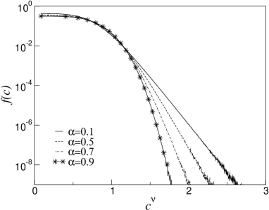
Figure 3: Free cooling with $(\theta=1,d=2,b=\nu=\sigma=0.5)$ at various values of $\alpha$.

Striking examples of the importance of sub-leading corrections are shown in Fig. 4, for a two-dimensional model with $\theta=1$, $\nu=2$, $\sigma=0$ and $\sigma=-0.5$. In these cases $b=2$, $b^{\prime}=1$ (for $\sigma=0$) and $b^{\prime}=3/2$ (for $\sigma=-0.5$). Comparison of the ”raw” DSMC data (dashed curve) with the dominant asymptotic prediction $\exp(-\beta c^{b})$ (dotted curve) shows no agreement. The reason is that the simulated $c-$values are not large enough. However, the solid curve (transformed DSMC data) $f(c)\exp[-\beta^{\prime}c^{b^{\prime}}]$ shows a striking agreement with the theory $\exp(-\beta c^{b})$, and demonstrates that the sub-leading corrections extend the validity of the asymptotic theory to much smaller $c-$values, thus enabling us to test the validity of theory, and establish the importance of the sub-leading corrections. Striking is the fact that such plots of $f(c)$ vs $c^{b}$ produces linear high energy tails (in spite of the importance of the sub-leading correction), which would then be well fitted with an effective value of $\beta$: $f(c)\sim\exp(-\beta_{\text{eff}}\,c^{b})$ (this is also the case in Fig. 2). As shown here, such an effective value can be markedly different from the true $\beta$, which indicates that any fitting procedure, aiming at computing $\beta$, is doomed to fail.

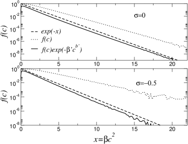
Figure 4: Comparison of the velocity distribution obtained from Monte Carlo (DSMC) simulations with the asymptotic predictions. For the Gaussian thermostat ($\theta=1,d=2,\alpha=0,\nu=2)$ at $\sigma=0$ (top) and $\sigma=-0.5$ (bottom) the exponents are $(b,b^{\prime},\chi)=(2,1,0)$ and $(2,1.5,0)$ respectively. DSMC data are plotted as $f(c)$ (dotted line) and $\exp[-\beta^{\prime}c^{b^{\prime}}]f(c)$ (solid line) vs $x=\beta c^{b}$, and compared with the theoretical prediction $e^{-x}$ (dashed line). Here $(\beta,\beta^{\prime})\simeq(1.087,1.359)$ for $\sigma=0$, and $\simeq(1.585,1.616)$ for $\sigma=-0.5$ have been measured in the DSMC simulations from their definition given in the text.

Figure 5 shows DSMC data for NF forcing with various values of $\nu$ and $\theta$. The simulations confirm the large-$c$ predictions, i.e. $\ln f(c)\sim-\beta c^{b}$, where $b=\nu+1-\theta$. Moreover, the dashed lines show the agreement with the prediction $\exp(-\beta c^{b})$ where the coefficient $\beta=2\langle|c|^{\theta+1}\rangle/[bpq\langle\langle g^{\nu+2}\rangle\rangle]$. For those parameters, the sub-leading corrections are negligible.

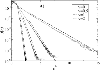
Figure 5: Negative friction with ($b=\nu+1-\theta,d=1,\alpha=0$). Plots show $f(c)$ vs. $c^{b}$ (A) for various values of $\nu$ at $\theta=0.5$, and (B) for various values of $\theta$ at $\nu=0.5$. The dashed lines correspond to the predictions $\exp(-\beta c^{b})$ vs. $c^{b}$ with $\beta$ calculated in each case by DSMC. The inset corresponds to a two-dimensional case ($\theta=0,\nu=2,\alpha=0$), showing $f(c)$ vs. $c^{b}$.

Regarding the soft sphere systems in stable NESS ($b>0$), either freely cooling or driven by Gaussian thermostats, we may conclude that the agreement between analytic and DSMC results for high energy tails is very good.

IV Marginal stability, power law tails

We now analyze the integral equation (13) for the threshold models ($b=0$; this fixes the exponent $\nu$ at the threshold). Marginal stability is a limiting property of a stable NESS as $b\to 0^{+}$, which occurs in states, driven either by white noise (see Ref.JSP-1 ) or by negative friction.

As we have seen in the previous section, the high energy tails for stable states ($b>0$) have the generic form $f(c)\sim\exp[-\beta c^{b}]$ with $\beta=\mathcal{B}_{\sigma}/b$, and sub-leading correction factors of similar structure. To illustrate how power law tails arise, we take the limit of $f(c)$ as $b\to 0^{+}$ using the relation $(c^{b}-1)/b\sim\ln c$. The result is,

$$f(c)\sim\lim_{b\to 0^{+}}c^{\chi}\exp[-\mathcal{B}_{\sigma}c^{b}/b]\equiv c^{\chi-\eta}.$$ (31)

Of course $(\chi-{\eta})$ is not the full exponent of the tail, because the exponential form above represents only the leading asymptotic behavior for $b>0$. For instance, any correction factor $\exp[-\beta^{\prime}c^{b^{\prime}}]$, where $b^{\prime}=H(b)\to 0$ as $b\to 0$, gives additional contributions to 31.

IV.1 Gaussian thermostat (NF: $\theta=1;b=\nu=0$)

Here the Maxwell molecules are the marginally stable model. To determine the full exponent of the power law tail we linearize the nonlinear integral equation 13 at the stability threshold around the ”thermal bulk part” of $f(c)$, using 15 and 16. We start with the simplest case of inelastic soft spheres, driven by a linear friction force ($\theta=1$).

Substitution of $f(c)=\delta({\bf c})+h(c)$ in the collision kernel of 13 yields to linear order in $h(c)$, $I(c|\delta+h)=-\Lambda h(c)$. The r.h.s. of 13 also simplifies, as $\langle\langle g^{\nu+2}\rangle\rangle=\langle\langle g^{2}\rangle\rangle=d$, and the resulting integral equation is,

$$\Lambda h=-\textstyle{\frac{1}{2}}\lambda_{2}\partial_{\bf c}\cdot({\bf c}f).$$ (32)

Inspection of this equation and 17 shows that the operators on left and right hand side, when acting on the right eigenfunction $1/c^{s+d}$ (recall that $\nu=0$) generate new powers of $c$. Solving the integral equation implies that one determines the value $s^{*}$ that makes both exponents equal, leading to the transcendental equation,

$$\lambda_{s}=\textstyle{\frac{1}{2}}s\lambda_{2}=spq\beta_{\sigma+2}.$$ (33)

Consequently, the solution of 32, which presents the asymptotic large-$c$ solution of 13, is the power law tail,

$$f(c)\sim h(c)\sim 1/c^{s^{*}+d}\qquad(c\gg 1).$$ (34)

If the transcendental equation has more solutions, then the largest root $s^{*}$ is the relevant one, because the energy $\langle c^{2}\rangle$, and possible moments $\langle c^{a}\rangle$ and $\langle\langle g^{a}\rangle\rangle$, appearing in the transcendental equations (see next subsection) must be finite, imposing $s^{*}>\max\{2,a\}$. So, the obvious solution of 33, $s^{*}=2$, has to be rejected. However the equation has a second solution with $s^{*}>2$, because $\lambda_{s}$ is a concave function of $s$. This can be seen directly from a graphical solution by adding in Fig. 1 the line $y(s)=\textstyle{\frac{1}{2}}s\lambda_{2}$. The numerical values of $s^{*}(\alpha)$, obtained from the numerical solution of 33, are shown in the inset of Fig. 6 for the two-dimensional system. The main plot shows the comparison of the DSMC measurements of $f(c)$ for this system compared to the theoretical predictions.

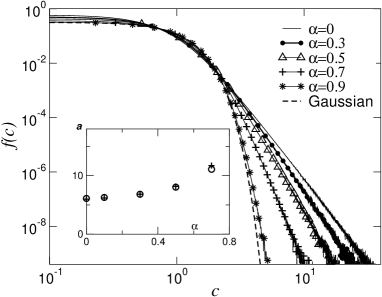
Figure 6: Power law tails in free cooling, obtained for the threshold model $(\theta=1,d=2,\sigma=1,b=\nu=0)$. The inset compares predicted and measured exponents. As $\alpha$ increases the exponent increases, and the curve tends to a Gaussian.

It is also instructive to consider the one-dimensional version of 33, which can be solved analytically. Then the eigenvalue 18 simplifies to $\lambda_{s}=1-q^{s}-p^{s}$, and 33 becomes, $1-q^{s}-p^{s}=spq$, with solutions $s^{*}=\{2,3\}$, and $s^{*}=3$ is the relevant one, and $f(c)\sim 1/c^{s^{*}+d}\sim 1/c^{4}$ in agreement with the exact solution $f(c)=(2/\pi)/[1+c^{2}]^{2}$, found in Rome .

For $d>1$ the transcendental equation can not be solved analytically, except in a few limiting cases, that we consider first. In the elastic limit ($\alpha\to 1$ or $q\to 0$) one only finds a meaningful solution of 33 by letting simultaneously $s\to\infty$ while keeping $sq=\xi=$ fixed. As $\beta^{\sigma+2}/\beta^{\sigma}=(\sigma+1)/(\sigma+d)$, and $\lambda_{s}/\beta^{\sigma}\to 1$ as $s\to\infty$ (see Fig. 1 or Eq.(3.12) in Ref.JSP-1 ), the transcendental equation 41 approaches $1\simeq\xi(1+\sigma)/(d+\sigma)$, yielding the solution,

$$s^{*}_{\sigma}=\xi/q\sim\left[({d+\sigma})/({1+\sigma})\right]/q\qquad(\alpha\to 1)$$ (35)

for general $\sigma$. In the elastic limit as $\alpha=1-2q\to 1$, the root $s^{*}_{\sigma}$ moves to  $\infty$  and the algebraic tail disappears, as required by consistency with the Maxwell distribution in the elastic limit. Using the large $s-$expansion of 33 it is straightforward to obtain additional sub-leading corrections.

Another case where the integral equation 33 can be solved analytically is at large dimensions KBN02 . To do so it is convenient to divide 33 by $\beta_{\sigma}$. As $d\to\infty$ its right hand side approaches $spq(1+\sigma)/d$. So, one finds only a meaningful solution by simultaneously letting $s\to\infty$ while keeping $x=s/d=$ fixed. To calculate $\lambda_{s}/\beta_{\sigma}$ from 18 in this coupled limit we use the relation,

$$\lim_{d\to\infty}{{}_{2}}F_{1}(\textstyle{-\frac{xd}{2},\frac{\sigma+1}{2};\frac{\sigma+d}{2}}|z)=\sum_{n=0}^{\infty}(\textstyle{\frac{1}{2}})_{n}(-xz)^{n}=\frac{1}{\sqrt{1+zx}},$$ (36)

where $(a)_{n}\equiv\Gamma(a+n)/\Gamma(a)$. This relation can be derived starting from the Gauss hyper-geometric series Abram+Stegun for ${}_{2}F_{1}(a,b;c|z)$ by taking the $(d\to\infty)$ limit term by term, and subsequently using the relation ${}_{2}F_{1}(a,b;b|z)=(1-z)^{-a}$. Then 33 for the present threshold model simplifies to,

$$1-\left(1+x(1-q^{2})\right)^{-(1+\sigma)/2}=xpq(1+\sigma).$$ (37)

For the $\sigma$-values, mostly considered in the literature, i.e. the model with $(\sigma=1)$ Math ; EB-JSP , and the mathematically convenient model $(\sigma=0)$ Maxwell ; EB-JSP , the above equation can be solved analytically. For the Maxwell model with $\sigma=1$ it is a quadratic equation, and for $\sigma=0$ it is a cubic equation. The root $x=0$ is not a solution of 33 because $\lambda_{s}$ in 18 holds only for $s>0$. The resulting $s^{*}_{\sigma}$ in 34 becomes in the coupled limit $d\to\infty,s\to\infty$ with $s/d=x=$ fixed,

$$s^{*}_{\sigma}=x^{*}_{\sigma}d\simeq\left\{\begin{array}[]{ll}\frac{d}{2q(1+q)}&\quad(\sigma=1)\\[5.69054pt] \frac{d}{q(1-q^{2})}[1+\textstyle{\frac{1}{2}}q+\sqrt{q(1+\textstyle{\frac{5}{4}q})}]&\quad(\sigma=0)\end{array}\right..$$ (38)

The exponent $s^{*}_{\sigma}+d$, obtained here, disagrees with the result of Ref. KBN02 in the sign in front of the square root. We note that the $\alpha-$dependence of $s^{*}_{0}$ and $s^{*}_{1}$ in the last equation is somewhat different at large $d$. The exponents in 35 and 38 agree in the respective limits $d\to\infty$ and $\alpha\to 1$.

Equation 33 can easily be solved numerically. For the Maxwell model with $\sigma=1$ the resulting exponents $s^{*}_{1}$ and $s^{*}_{0}$ as a function of $\alpha$ for various $d$ are plotted as $s^{*}_{1}/d$ and $s^{*}_{0}/d$ in Fig. 7. As shown in the inset of Fig. 6, the agreement with DSMC simulations is very good.

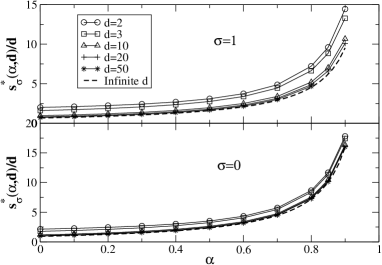
Figure 7: $s^{*}_{\sigma}(\alpha,d)/d$ vs $\alpha$ for the two variants of $d-$dimensional Maxwell models, i.e. (top) with $(\sigma=1,\nu=0)$ and (bottom) with $(\sigma=\nu=0)$. The dashed lines correspond to the analytic results 38 for large $d$.

Most results of this subsection, applying to Maxwell models ($\nu=0$), have been derived already in the literature using an entirely different mention, namely by Fourier transformation with respect to the velocity variables. The Fourier transform method can only be applied to Maxwell models ($\nu=0)$ where the microscopic collision frequency is independent of the relative velocity $g$, leading to a collision kernel $I(c|f)$ that is a convolution product in velocity space. It simplifies to an ordinary product after Fourier transformation. The method can not be generalized to inelastic soft sphere models with $\nu\neq 0$. Our method on the other hand can be applied for all values of $\nu$.

IV.2 Nonlinear negative friction
(NF: $\theta\geq 0;b=\nu+1-\theta=0$)

In this case, the threshold model is the soft sphere mode with $b=0$ or $\nu=\theta-1$. The corresponding scaling equation for the high energy tail is obtained by setting $\nu=\theta-1$ in 13, and reads,

$$I(c|\delta+h)=-\Lambda h=\textstyle{\frac{1}{2}}\lambda_{2}\Gamma(\theta){\bf\partial}\cdot(\hat{{\bf c}}c^{\theta}h),$$ (39)

where we have defined the ratio of the moments $\Gamma(\theta)$ as,

$$\Gamma(\theta)\equiv\frac{\langle\langle g^{\theta+1}\rangle\rangle}{2\langle c^{\theta+1}\rangle}.$$ (40)

This quantity should not be confused with the Euler Gamma function. We also note that $\Gamma(\theta)$ is unknown a priori, as it depends on the full unknown scaling form $f(c)$ with $c\in(0,\infty)$. Inspection of 39 shows again that the operators on left and right hand side of 39, when acting on the right eigenfunction $1/c^{s+d+\nu}$ with $\nu=\theta-1$, will produce new powers of $c$, and one determines the value $s^{*}$, that makes both exponents equal, by solving the transcendental equation,

$$\lambda_{s}=\textstyle{\frac{1}{2}}s\lambda_{2}\Gamma(\theta)=spq\beta_{\sigma+2}\Gamma(\theta).$$ (41)

We recall that $\lambda_{s}$ is the same for all inelastic soft sphere models. We further note that $\Gamma(\theta=1)=1$, as can be verified from 40 and the normalization $\langle c^{2}\rangle=d/2$, and we recover the transcendental equation 33 for linear friction.

Denoting the relevant root of 41 by $s^{*}_{\sigma}$ the solution of 39 is the right eigenfunction of $\Lambda$ with eigenvalue $\lambda_{s^{*}_{\sigma}}$, i.e.

$$f(c)\sim h(c)\sim c^{-s^{*}_{\sigma}-d-\theta+1}.$$ (42)

So at the stability threshold for driving by nonlinear friction ($\nu=\theta-1$), there exists again a power law tail in the scaling solution of the Boltzmann equation for soft sphere models, provided 41 does indeed have a real positive solution.

Extracting the largest root from 41 is somewhat more complicated than in equation 33, because of the unknown factor $\Gamma(\theta)$. Even for $d=1$ there are no simple exact solutions. To obtain $\Gamma(\theta)$ we determine the moments in 40 and their ratio $\Gamma(\theta)$ by direct DSMC measurements. The inset of Fig. 8 shows $\Gamma(\theta)$ resulting from these measurements at $\alpha=0$ in two dimensions. The plot shows that $\Gamma(\theta)$ is an approximately linear function increasing with $\theta$. At this point, it is noteworthy that a Gaussian ansatz for the velocity distribution yields $\Gamma(\theta)=2^{(\theta-1)/2}$. This provides an excellent approximation (not shown) , which also coincides with the exact value at $\theta=-1$. There the linear approximation is slightly off. However, in the physically relevant range, $\theta\in[0,1]$, the linear approximation is slightly better. The following analytical results confirm this trend: $\Gamma=\textstyle{\frac{1}{2}},1$ for $\theta=-1,1$ respectively. The resulting $\Gamma(\theta)$ is used as a known input parameter in 41.

Once $\Gamma(\theta)$ is known from DSMC measurements, one can construct a simple graphical method for solving 41 and classifying its possible solutions for different values of $\theta$ and $\alpha$. Here we discuss only the $\nu$ models with $\sigma=1$. This is done by plotting in Fig. 8 for a fixed value of $\alpha$ the curve, $y_{1}(s)=\lambda_{s}/\beta_{1}$ (l.h.s. of 41), and the straight lines, $y_{2}(s)=[2pq\Gamma(\theta)/(d+1)]s$ (r.h.s. of 41, as follows from $\beta_{3}/\beta_{1}=2/(d+1)$), for different values of $\theta$, and determine the largest intersection point. Here $\Gamma_{c}$ defines the slope of the line, $y=[2pq\Gamma_{c}/(d+1)]s$, through the origin, that is tangent to curve $\lambda_{s}$. The largest intersection point of the eigenvalue curve with the line, labelled $\Gamma(\theta=1)=1$, represents the graphical solution for the linear friction case, and the relevant root $s^{*}(\alpha)$ has already been obtained in Fig. 6 for two dimensions EB-JSP ; EB-SpringII . For the nonlinear case we obtain the following scenario. As $\theta$ decreases from 1 to 0, the ratio $\Gamma(\theta)$ decreases from 1 to some value $\Gamma(0)>1/2$, and the largest root $s^{*}_{+}=s^{*}_{+}(\theta,\alpha)$ grows from $s^{*}$ to some value $s^{*}_{+}(0,\alpha)$. As $\theta$ grows larger than 1, $\Gamma(\theta,\alpha)$ increases from 1 to $\Gamma_{c}(\alpha)$, and the largest root $s^{*}_{-}=s^{*}_{-}(\theta,\alpha)$ decrease from $s^{*}$ to $s^{*}_{c}$, as shown in Fig. 8. For $\Gamma(\theta)>\Gamma_{c}$ the root of the transcendental equation becomes complex. The corresponding tail with an oscillatory pre-factor is no longer everywhere non-negative, and thus becomes unphysical.

Figure 8: NF at ($d=2$, $\sigma=1$, $\nu=\theta-1$, $\alpha=0$). Graphical solution of 41 for the marginally stable NF driven soft sphere model. The concave curve represents the eigenvalue $y_{1}(s)=\lambda_{s}(1)/\beta_{1}$ (solid line) and the straight lines represent $y_{2}(s)$ (see text) for different values of $\Gamma(\theta)$, labelled from bottom to top by $\Gamma_{n}(n=0,1,2)$. The inset shows $\Gamma(\theta)$ versus $\theta$ as obtained from DSMC measurements. The slope of the tangent line is labeled by $\Gamma_{c}$. The largest intersection point corresponds for a given value of $\Gamma(\theta)$ to the root $a_{n}(\sigma)$, which determines the power law tail $f(c)\sim 1/c^{a+d+\theta-1}$.

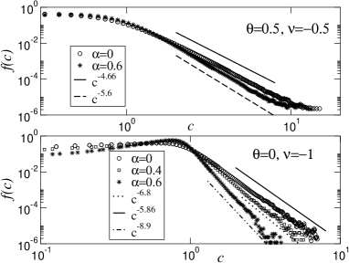
Figure 9: NF at stability threshold ($d=1,b=\nu+1-\theta=0$). (top): $(\theta,\nu)=(0.5,-0.5)$; (bottom): $(\theta,\nu)=(0,-1)$. The lines are the predicted power law tails, $f(c)\sim 1/c^{a+d+\theta-1}$, following from the construction discussed in Fig. 8.

Figure 10: NF at stability threshold ($d=2,b=\nu+1-\theta=0$). (top): $\alpha=0$ and $(\theta,\nu)=\{(1,0),(0.5,-0.5),(0.1,-0.9)\}$; (middle): $(\theta,\nu)=(0.5,-0.5)$ and $\alpha=\{0.0,0.3,0.5\}$; (bottom): $(\theta,\nu)=(1.1,0.1)$ and $\alpha=\{0.1,0.5,0.6\}$. The plots show the predicted power law tails, $f(c)\sim 1/c^{E}$, as dashed lines with exponents $E=a+d+\theta-1$, where $a$ is calculated from the transcendental equation 41 using the measured values of $\Gamma(\theta)$ (see also Fig. 8) . The predicted exponents are: (top): $E=\{6.0,6.8,7.75\}$ ; (middle): $E=\{6.8,7.8,9.4\}$; (bottom): $E=\{6.0,8.0,9.2\}$. These exponents show very good agreement with DSMC data.

We finally present a comparison of our analytical predictions with the result of DSMC simulations for several parameter values in Figs. 9 and 10. Due to the marginally stable character of the NESS, simulations are quite difficult and time-consuming. Nevertheless, an excellent agreement is obtained for all parameter values. Note that the values of the power-law exponents are large so that a direct fit to power-law forms would not be very precise, and could not exclude other fitting forms (since at most one decade in $c$ is covered).

V Inelastic BGK models

In this section we study a simple inelastic BGK (Bhatnagar - Gross - Krook) model for homogeneous velocity relaxation BMD ; EB-SpringII , which only takes the most essential features of the complex nonlinear collision operator into account. The goal is to understand how much of the rich behavior of the Boltzmann equation, described in the present paper and in JSP-1 , is preserved in such a linear model. The analytic results of the previous sections, and of Refs. JSP-1 ; EPL ; QE , are restricted to asymptotic solutions, which can be applied directly to V. The BGK kinetic equations allow to go further, since they reduce to simple linear first and second order inhomogeneous ODE’s, which can be solved exactly, at least for systems that are freely cooling, or equivalently driven by linear negative friction, as well as for systems driven by white noise. Although the present paper is mainly dealing with nonlinear negative friction, we restrict ourselves to the Gaussian thermostat (linear friction) and also discuss white noise driving for completeness. The exact solution of the BGK model with the full nonlinear friction is not known.

In a crude scenario for relaxation without energy input, the velocity distribution $F(v,t)$ relaxes towards a Maxwellian with shrinking width $\alpha v_{0}(t)$, at a rate $\propto v^{\nu}_{0}(t)$. The width, proportional to $\alpha$, mimics the role of the coefficient of restitution, which reduces the typical velocity in an inelastic collision by a factor $\alpha$. With a constant supply of energy, the system can reach a NESS, and the global evolution can be modelled by the BGK-type kinetic equation,

Figure 11: BGK in one and two dimensions for FC: log-log plot showing the power-law tails.

$$\partial_{t}F(v,t)-D\partial_{{\bf v}}^{2}F(v,t)=I(v|F)$$

$$I(v|f)=-v_{0}^{\nu}(t)[F(v,t)-F_{0}(v,t)]$$

$$F_{0}(v,t)=(\alpha v_{0})^{-d}\phi(v/\alpha v_{0}(t)),$$ (43)

where $\phi(c)=\pi^{-d/2}\exp[-c^{2}]$ is the Maxwellian. If $F(v,t)$ is rapidly approaching the scaling form 5, the rescaled collision kernel, $I(v|F)=v_{0}^{\nu-d}I(c|f)$, takes the form,

$$I(c|f)=-f(c)+\alpha^{-d}\phi(c/\alpha).$$ (44)

We note that the collision kernel does not show any $\nu$-dependence. This is similar to Maxwell models, where the collision frequency is independent of the microscopic velocities of the colliding particles. The time evolution of $v_{0}(t)$ in free cooling and in the WN (white noise) case obeys equations of motion, similar to 7-11. Because for inelastic soft spheres the rhs is also proportional to $1-\alpha^{2}$, the discussion about stability of the granular temperature $T(t)\sim v^{2}_{0}(t)$ is the same as in free cooling and WN driving JSP-1 ; EPL , and the same applies to Haff’s homogeneous cooling law, $v^{2}_{0}(t)\sim t^{-2/\nu}$.

In the free cooling case ($D=0$) the energy equation becomes, $\dot{v}_{0}=-2pqv_{0}^{\nu+1}$. Inserting then the scaling ansatz 5 in V yields,

$$cf^{\prime}+(d+a)f=\frac{a}{\alpha^{d}}\phi\left(\frac{c}{\alpha}\right);\qquad a=2/(1-\alpha^{2})$$ (45)

Its exact solution is (see also BMD ; EB-SpringII ),

$$f(c) = \frac{a\alpha^{a}}{\pi^{d/2}}\left(\frac{1}{c^{d+a}}\right)\int_{0}^{\alpha c}du\,u^{d+a-1}e^{-u^{2}}$$ (46)

$$\sim \frac{a\alpha^{a}\Gamma\left(\frac{d+a}{2}\right)}{2\pi^{d/2}}\left(\frac{1}{c^{d+a}}\right)\quad(c\gg 1)$$

This solution, including its high energy tail (see Fig. 11), is independent of the exponent $\nu$. A similar heavily overpopulated power law tail, $f(c)\sim 1/c^{d+a}$ with $d>1$, is also found in the freely cooling Maxwell model. There the exponent $a(\alpha)$ takes in the elastic limit ($\alpha\to 1$) the very similar form $a\simeq 4d/(1-\alpha^{2})$ (compare 45). We also note that the $\alpha$-dependence of the power law exponent in the BGK model is essentially the same as for higher dimensional Maxwell models JSP-1 , and similar to 38 for NF driving. However, in the general class of inelastic soft sphere models with collision frequency $g^{\nu}$ and $\nu>0$ (hard scatterers), the tail is not a heavily overpopulated power law tail, but a lightly overpopulated stretched exponential, $f(c)\sim\exp[-\beta c^{b}]$ with $b=\nu>0$. The BGK models describe quite well the features of the soft scattering models, but are totally missing the more effective randomization caused by the high speed particles present, in models with positive $\nu$.

Let us now turn to the case of white noise driving in the BGK model of Eqs. V. Again the energy balance equation is the same as 7 for soft spheres. So all BGK models with $\nu>-2$ have a stable attracting fixed point $v_{0}(\infty)$, and the integral equation has a rescaled form, analogous to 13,

$$f^{\prime\prime}(c)+\frac{d-1}{c}f^{\prime}(c)-2af(c)=-\frac{2a}{\alpha^{d}}\phi\left(\frac{c}{\alpha}\right).$$ (47)

Here a prime on $f$ denotes a derivative with respect to its argument $c$. Eq. 47 shows that $f(c)$ is independent of the model parameter $\nu$ and of the noise strength $D$. The equation can be solved exactly, and the two integration constants are fixed by the normalizations 6. For all values of $d$ we make the transformation

$$f(c)=\alpha^{-d}y(\beta c);\quad b=\textstyle{\frac{1}{2}}\beta\alpha;\quad\beta=\sqrt{2a}=2/\sqrt{1-\alpha^{2}},$$ (48)

where $y$ is a function to be determined. The resulting equation for $y$ can be solved: the one-dimensional BGK model has the exact solution

$$y(x)=\textstyle{\frac{1}{2}}{b\exp[b^{2}]}\left[e^{x}{\rm erfc}(b+\frac{x}{2b})+e^{-x}{\rm erfc}(b-\frac{x}{2b})\right].$$ (49)

Using the properties of the complementary error function ${\rm erfc}(z)$ one can verify that the first term inside $[\cdots]$ decays for $x\to\pm\infty$ as $\exp[-x^{2}/4b^{2}]$ and the second one as $2\exp[-x]$, yielding an exponential tail,

$$f(c)\sim\textstyle{\frac{1}{2}}\beta\exp[b^{2}]e^{-\beta|c|}\qquad(c\gg 1).$$ (50)

Similarly we find in the two-dimensional case for the solution satisfying the normalizations 6, i.e.

$$y(x) = \frac{1}{\pi}K_{0}(x)\int_{0}^{x}zdz\exp[-z^{2}/4b^{2}]I_{0}(z)$$ (51)

$$+ \frac{1}{\pi}I_{0}(x)\int_{0}^{x}zdz\exp[-z^{2}/4b^{2}]K_{0}(z),$$

where $I_{0}(x)$ and $K_{0}(x)$ are Bessel functions with imaginary argument Abram+Stegun . The exact solutions 46, 49 and 51 have been obtained by K. Shundyak . At large $x$ we have $K_{0}(x)\sim e^{-x}\sqrt{\pi/2x}$ and $I_{0}(x)\sim\exp[-x^{2}/4b^{2}]$, yielding the high energy tail,

$$f(c)\sim\frac{e^{\alpha^{2}/(1-\alpha^{2})}}{\sqrt{\pi}(1-\alpha^{2})^{3/2}}\left(\frac{e^{-\beta c}}{\sqrt{c}}\right).$$ (52)

For higher dimensions $(d>2)$ we only quote the asymptotic solution,

$$f(c)\sim c^{1-d/2}e^{-\beta c}\ ,$$ (53)

which may also be obtained directly from 47 by neglecting the inhomogeneity, i.e. the gain term $I_{\mbox{gain}}$ $\sim\exp[-c^{2}/\alpha^{2}]$.

Figure 12: BGK with WN driving, in one and two dimensions, showing the exponentially decreasing tails.

Comparison with the results of JSP-1 for the WN-driven soft sphere models shows that the large-$c$ behavior is exactly the same as that of the Maxwell model ($\nu=0$), but the scaling solutions, displayed in Fig. 12, are independent of $\nu$ (since Eq. 47 is itself independent of $\nu$), whether the scaling solution is a stable attracting state of a hard scattering model, or an unstable repelling state state of a soft scattering model. It shows therefore again that the BGK model is inadequate to model hard interactions.

In summary, the simple linear BGK model, although displaying interesting features, such as power-law velocity distribution tails, is far from being able to capture the rich behavior of the Boltzmann equation, in particular it fails for hard interactions ($\nu>0)$.

VI Concluding remarks

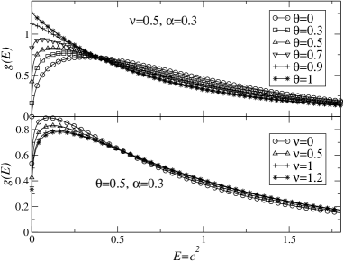
Figure 13: Isobestic points as either $\theta$ is changed at constant $\nu$ and $\alpha$, or as $\nu$ is changed at constant $\theta$ and $\alpha$. Top: $d=1$; Bottom $d=2$ (in 2 dimensions we plot the distribution of the energy $E=c^{2}$).

Within the framework of the nonlinear Boltzmann equation coupled to stochastic or deterministic driving forces and ’heat’ baths, we have studied a general class of inelastic soft sphere models. Our approach encompasses a broad class of previously introduced models, from hard scatterers like inelastic hard spheres (and even very hard spheres Phys-Rep-ME ), to soft scatterers like Maxwell molecules, and even softer ones with $\nu<0$, where $\nu$ governs the dependence of collision frequency on relative velocity $g$ through a term $g^{\nu}$.

We have shown that the velocity distribution $f(c)$ has a stretched exponential tail $\propto\exp(-c^{b})$, when the non-equilibrium steady state is an attractive fixed point of the dynamics. In certain regions of model parameters ($\nu,\alpha,\theta$) where $\alpha$ denotes the restitution coefficient and $\theta$ is a friction parameter, we have reported important sub-leading corrections, where $f(c)$ is found to be of the form $c^{\chi}\exp(-\beta v^{b}+\beta^{\prime}v^{b^{\prime}})$. The comparison with high-precision numerical solutions of the Boltzmann equation, obtained through Monte Carlo simulations (DSMC scheme), shows that neglecting these sub-leading corrections in a fitting procedure can lead to erroneous estimates of $\beta$. Algebraic distributions emerge in cases of marginal stability ($b=0$), and we have calculated the corresponding power law exponents. The high accuracy of our DSMC simulations have enabled us to verify the theoretical predictions for a wide range of parameter values.

The models studied here are partially amenable to analytical progress, but some features resist understanding. We conclude here by reporting one such feature, that is illustrated in Fig. 13. We observe that all steady state rescaled velocity distributions, at fixed $\nu$ and varying $\theta$, pass through a common point. A similar property seems to hold when $\theta$ is held fixed, and varying $\nu$. Such points, that can be coined “isobestic”, have already been observed in a different context (see e.g. section IV-E in reference PTD ), where their occurrence could not be rationalized.

Acknowledgements We would like to thank a referee for valuable suggestions.

References

- (1) H.M. Jaeger, S.R. Nagel, and R.P. Behringer, Rev. Mod. Phys. 68, 1259 (1996).
- (2) Theory of Granular Gas Dynamics, Th. Pöschel and N.V. Brilliantov (Eds) (Springer-Verlag, Berlin, 2003).
- (3) A. Barrat, E. Trizac, M.H. Ernst, J. Phys. Condens. Matter 17, S2429 (2005).
- (4) T. Pöschel, S. Luding, eds., Granular Gases (Springer, Berlin, 2001), Lecture Notes in Physics 564.
- (5) T. Pöschel, N. Brilliantov, eds., Granular Gas Dynamics (Springer, Berlin, 2003), Lecture Notes in Physics 624.
- (6) J. S. Olafsen and J. S. Urbach, Phys. Rev. Lett. 81, 4369 (1998); W. Losert, at al, Chaos 9, 682 (1999); F. Rouyer and N. Menon, Phys. Rev. Lett. 85, 3676 (2000); D.L. Blair and A. Kudrolli, Phys. Rev. E 64, 050301(R) (2001); I.S. Aranson and J.S. Olafsen, Phys. Rev. E 66, 061302 (2002); S. Moka and P.R. Nott, Phys. Rev. Lett.95,068003 (2005).
- (7) A. Prevost, D. A. Egolf, and J. S. Urbach, Phys. Rev. Lett. 89, 084301 (2002).
- (8) A. Barrat and E. Trizac, Eur. Phys. J. E 11, 99 (2003).
- (9) K. Kohlstedt, A. Snezhko, M. V. Sapozhnikov, I. S. Aranson, J. S. Olafsen, and E. Ben-Naim, Phys. Rev. Lett. 95, 068001 (2005).
- (10) A. Goldshtein and M. Shapiro, J. Fluid Mech. 282, 75 (1995).
- (11) J.J. Brey, J.W. Dufty, C.S. Kim and A. Santos, Phys.Rev.E 58, 4638 (1998); J.J. Brey, D. Cubero and M.J. Ruiz-Montero, Phys. Rev. E 59 1256 (1999); J.J. Brey and M.J. Ruiz-Montero, Phys. Rev. E 67, 021307 (2003).
- (12) A. Puglisi, V. Loreto, U.M.B. Marconi, A. Petri, A. Vulpiani, Phys. Rev. Lett. 81, 3848 (1998).
- (13) A. Baldassarri, U. Marini Bettolo Marconi, and A. Puglisi, Europhys. Lett. 58, 14 (2002); A. Baldassarri, U. Marini Bettolo Marconi, and A. Puglisi, Math. Mod. Meth. Appl. S. 12, 965 (2002).
- (14) A. Barrat, E. Trizac and J.N. Fuchs, Eur. Phys. J E 5, 161 (2001).
- (15) T.P.C. van Noije and M.H. Ernst, Granular Matter 1, 57 (1998).
- (16) J.M. Montanero and A. Santos, Granular Matter 2, 53 (2000).
- (17) R. Cafiero, S. Luding and H.J. Herrmann, Phys. Rev. Lett. 84, 6014 (2000).
- (18) S.J. Moon, M. D. Shattuck, and J. B. Swift, Phys. Rev. E 64, 031303 (2001);
- (19) A. Santos and J.W. Dufty, Phys. Rev. Lett. 86 4823 (2001).
- (20) E. Ben-Naim and P.L. Krapivsky, Phys. Rev. E 61, R5 (2000); ibidem 66, 1309 (2002).
- (21) P.L. Krapivsky and E. Ben-Naim, J. Phys. A 35, L147 (2002).
- (22) M.H. Ernst and R. Brito, Europhys. Lett. 58:182(2002); J. Stat. Phys.109, 407 (2002);
- (23) M.H. Ernst and R. Brito, Phys. Rev. E 65, 04301 (2002).
- (24) A.V. Bobylev, C. Cercignani and G. Toscani, J. Stat. Phys. 111, 403 (2003); I.M. Gamba, V. Panferov and C. Villani, Comm. Math. Phys. 246, 503 (2004).
- (25) A. Barrat, T. Biben, Z. Rácz, E. Trizac, and F. van Wijland, J. Phys. A: Math. Gen. 35, 463 (2002).
- (26) T. Biben. Ph. A. Martin and J. Piasecki, Physica A 310, 308 (2002); E. Barkai, J. Stat. Phys. 115, 1537 (2004).
- (27) D. ben-Avraham, E. Ben-Naim, K. Lindenberg, and A. Rosas, Phys.Rev. E 68, 050103 (2003).
- (28) O. Herbst, P. Müller, M. Otto, and A. Zippelius, Phys. Rev. E 70, 051313 (2004).
- (29) J.S. van Zon and F. C. MacKintosh, Phys. Rev. E, 72, 051301 (2005).
- (30) Y. Srebro and D. Levine, Phys. Rev. Lett. 93, 240601 (2004).
- (31) E. Ben-Naim, B. Machta and J. Machta, Phys. Rev. E 72, 021302 (2005); E. Ben-Naim and J. Machta, Phys. Rev. Lett. 94, 138001 (2005).
- (32) M.H. Ernst, E. Trizac and A. Barrat, J. Stat. Phys. 124, 549 (2006).
- (33) M.H. Ernst, E. Trizac and A. Barrat, Europhys. Lett. 76, 56 (2006).
- (34) M.H. Ernst, Phys. Rep. 78,1 (1981).
- (35) T.P.C. van Noije, M.H. Ernst, E. Trizac and I. Pagonabarraga, Phys. Rev. E 59, 4326 (1999); I. Pagonabarraga, E. Trizac, T.P.C. van Noije and M.H. Ernst, Phys. Rev. E 65, 011303 (2002).
- (36) G. Bird, Molecular Gas Dynamics and the Direct Simulation of Gas Flows (Clarendon, Oxford, 1994).
- (37) M. Abramowitz and I. Stegun, Handbook of Mathematical Functions (Dover Publications, Inc. New York, 1965).
- (38) A. Barrat, E. Trizac, and M.H. Ernst, J.Phys.A: Math. Theor. 40, 4057 (2007).
- (39) J.J. Brey, F. Moreno, J.W. Dufty, Phys. Rev. A 54, 445 (1996).
- (40) M.H. Ernst and R. Brito, See PoschelBrill and cond-mat/0304608.
- (41) J. Piasecki, E. Trizac, and M. Droz, Phys. Rev. E 66, 066111 (2002).