Characteristic Time and Maximum Mixedness: Single Mode Gaussian States in Dissipative Channels

Abstract

We derive an upper limit for the mixedness of single bosonic mode gaussian states propagating in dissipative channels. It is a function of the initial squeezing and temperature of the channel only. Moreover the time at which von Neumann’s entropy reaches its maximum value coincides with that of complete loss of coherence, thus defining a quantum-classical transition.

I Introduction

The search for quantum squeezed states of light began in the 1950’s with the pioneering works of Senitzky, Plebanski and others senitzky ; husimi ; plebanski ; epstein . The recent and rapid development of quantum information has greatly stimulated research on nonclassical states of light. They play an important role in quantum information processing with continuous variables braustein1 , in which information is encoded in two conjugate quadratures of an optical field mode. Moreover, quantum mechanical squeezing of optical fields represents a means to improve the precision of measurements below the standard quantum noise detection. Also, squeezed states may be used as an entanglement source: for example, combining two squeezed states at a beam splitter creates an entangled two-mode squeezed state, as required for quantum teleportation bennett or dense coding schemes braustein2 . On the experimental side, a proposed scheme jaromir1 for measuring squeezing, purity and entanglement of Gaussian squeezed states (GSS) of light was realized recently jaromir2 .

As is well known, dissipative environments tend to render quantum features unobservable. Dissipative dynamics of quantum systems have been investigated, both theoretically caldeira1 ; caldeira ; zurek ; cavalcanti ; lee ; han ; subpoissonian ; manko ; lages ; rossi ; saraceno ; karen ; knight1 ; oliveira ; knight3 ; knight2 ; dodonov ; ozorio ; italianos1 ; italianos ; marian2 and experimentally paris ; paris1 ; walborn ; experimental ; experimental1 . Understanding the factors which limit the visibility and also the time scales of quantum properties (QP) is of interest if they are to be used in the context of quantum computation or foundations of quantum theory, e.g. the quantum - classical border.

In the present contribution we analytically derive two essential ingredients for the visibility of QP (in the context of to a Caldeira-Legget type environment): (i) an upper limit for the mixedness of the initial single mode bosonic GSS and (ii) a time scale for (the observables) squeezing and oscillations in photon number distributions. These two conditions, considered together, convey in simple terms the relevant control parameters in an experiment involving such states.

II Single mode bosonic Gaussian States and their dissipative dynamics

In this work we deal with single mode displaced, squeezed, mixed Gaussian States. This class of states can always be put in the form

$$\hat{\rho}_{G}=\mathcal{D}(\alpha_{0})\mathcal{S}(r_{0},\phi_{0})\hat{\rho}_{\nu_{0}}\mathcal{S}^{\dagger}(r_{0},\phi_{0})\mathcal{D}^{\dagger}(\alpha_{0})$$ (1)

where $\mathcal{D}(\alpha)$ is the displacement operator, $\mathcal{S}(r,\phi)$ is the squeezing operator and $\hat{\rho}_{\nu}$ is the thermal density operator whose degree of mixedness is given by $\operatorname{tr}[a^{\dagger}a\rho_{\nu}]=\nu$. The subscripts 0 denote initial values. More explicitly we have

$$\mathcal{D}(\alpha) = \exp(\alpha a^{\dagger}-\alpha^{*}a)$$ (2)

$$\mathcal{S}(r,\phi) = \exp\Big{(}\frac{1}{2}r\mathrm{e}^{i\phi}a^{\dagger 2}-\frac{1}{2}r\mathrm{e}^{-i\phi}a^{2}\Big{)}$$ (3)

$$\hat{\rho}_{\nu} = \frac{1}{1+\nu}\exp\Bigg{(}\ln\Big{(}\frac{\nu}{\nu+1}\Big{)}a^{\dagger}a\Bigg{)}.$$ (4)

The dissipative dynamics is taken to be the following master equation (we will work in units such that $\hbar=1$)

$$\dot{\rho}=\mathcal{L}\rho$$ (5)

where $\mathcal{L}$ is the Liouvillian super-operator :

$$\mathcal{L} = -i\omega[a^{\dagger}a,\bullet]+k(\bar{n}_{B}+1)(2a\bullet a^{\dagger}-a^{\dagger}a\bullet-\bullet a^{\dagger}a)+$$ (6)

$$+k~{}\bar{n}_{B}(2a^{\dagger}\bullet a-aa^{\dagger}\bullet-\bullet aa^{\dagger}),$$

known to yield good quantitative agreement with data from quantum optics (the $\bullet$ indicates where the super-operator acts). In equation (5) $\omega$ stands for the field frequency, $\bar{n}_{B}$ is the average number of thermal photons and $k$ the dissipation constant.

The analytical solution of (5) for states of the form (1) are given by serafini

$$\alpha(t) = \alpha_{0}\mathrm{e}^{-(i\omega+k)t}$$ (7)

$$\phi(t) = \phi_{0}-2\omega t$$ (8)

$$\nu(t) = \sqrt{x^{2}(t)-\Big{(}(\nu_{0}+\frac{1}{2})\sinh(2r_{0})\mathrm{e}^{-2kt}\Big{)}^{2}}-\frac{1}{2}$$

$$x(t) = \Big{(}\nu_{0}+\frac{1}{2}\Big{)}\cosh(2r_{0})\mathrm{e}^{-2kt}+\Big{(}\overline{n}_{B}+\frac{1}{2}\Big{)}(1-\mathrm{e}^{-2kt})$$

$$r(t) = \frac{1}{4}\ln\Bigg{(}\frac{(\nu_{0}+\frac{1}{2})\mathrm{e}^{2r_{0}}+(\overline{n}_{B}+\frac{1}{2})(\mathrm{e}^{2kt}-1)}{(\nu_{0}+\frac{1}{2})\mathrm{e}^{-2r_{0}}+(\overline{n}_{B}+\frac{1}{2})(\mathrm{e}^{2kt}-1)}\Bigg{)}.$$

Now we use a well known property of Gaussian states that allows us to obtain an analytical expression for von Neumann’s entropy agarwal : any Gaussian state is completely determined by the mean values of position and momentum operators as well as their quadratures. The property we have in mind is the determinant of the covariance matrix

$$D(t) =\textrm{Det}\begin{pmatrix}\sigma_{pp}&\sigma_{qp}\\ \sigma_{qp}&\sigma_{qq}\end{pmatrix}$$ (12)

where $\sigma_{xy}=\frac{1}{2}\operatorname{tr}[{\hat{\rho}}\left\{\hat{x},\hat{y}\right\}]-\operatorname{tr}[\hat{x}\hat{\rho}]\operatorname{tr}[\hat{y}\hat{\rho}]$. It is easy to show that, for a single mode GSS:

$$D(t)=\Big{(}\nu(t)+\frac{1}{2}\Big{)}^{2}$$ (13)

and

$$S[\rho_{\nu}(t)]=(\nu(t)+1)\ln\big{(}\nu(t)+1\big{)}-\nu(t)\ln\big{(}\nu(t)\big{)}$$ (14)

where $S[\rho_{\nu}(t)]=-\operatorname{tr}[\rho_{\nu}\ln\rho_{\nu}]$ is the von Neumann entropy. Note that the coherence content of the time evolved GSS is independent of the displacement $\alpha(t)$ and the squeezing phase $\phi(t)$. The QP contained in a GSS are its squeezing and oscillations in photon number distribution. During the time interval when such properties are visible one finds an increase in entropy which afterwards decays to the purely Gaussian vacuum state (for zero temperature). In figure (1) we illustrate how the initial mixedness of the GSS influences the visibility of quantum coherence. It shows the entropy for a pure ($\nu_{0}=0$) and a mixed Gaussian state ($\nu_{0}=3$). In the present case the time scale for both squeezing and oscillations in photon number distributions coincides with the time at which the von Neumann entropy attains its maximum value.

A physical understanding of the dynamical process is best afforded by the Wigner function (WF). For a GSS we get

$$W(x,p) = \sum_{l}\frac{1}{\pi}\frac{\nu^{l}}{(\nu+1)^{l+1}}(-|F_{3}|)^{l}\cdot L_{l}\Big{[}2\Big{(}\frac{(x-x_{0})^{2}}{F_{4}^{2}}+\frac{(F_{4}F_{5})^{2}}{4}\Big{)}\Big{]}\cdot$$ (15)

$$\cdot\frac{F_{4}}{|F_{1}|}\mathrm{e}^{-\frac{(x-x_{0})^{2}}{F_{4}^{2}}}\mathrm{e}^{-\frac{(F_{4}F_{5})^{2}}{4}},$$

where $L_{l}(x)$ is the Laguerre function of $l$ order (and argument $x$) and we define nieto

$$F_{1} = \cosh r+\mathrm{e}^{i\phi}\sinh r$$

$$F_{2} = \frac{1-i\sin\phi\sinh r(\cosh r+\mathrm{e}^{i\phi}\sinh r)}{(\cosh r+\cos\phi\sinh r)(\cosh r+\mathrm{e}^{i\phi}\sinh r)}$$

$$F_{3} = \frac{\cosh r+\mathrm{e}^{-i\phi}\sin\phi\sinh r}{\cosh r+\mathrm{e}^{i\phi}\sin\phi\sinh r}$$

$$F_{4} = \sqrt{\cosh^{2}r+\sinh^{2}r+2\cos\phi\cosh r\sinh r}$$

$$F_{5} = 2(p+p_{0})-i(x-x_{0})(F_{2}^{*}-F_{2}).$$ (16)

The Wigner function above can also be written in a closed Gaussian form (since the dynamics do not change its Gaussian character):

$$W(x,p) = \frac{1}{\pi(\nu+\frac{1}{2})}\exp\Big{\{}-\frac{\cosh(2r)}{2\nu+1}\left[(1-\tanh(2r)\cos\phi)x^{2}+(1+\tanh(2r)\cos\phi)p^{2}\right]+$$ (17)

$$+\frac{\sin\phi\sinh(2r)}{\nu+\frac{1}{2}}xp\Big{\}}.$$

At time zero the WF shows apparent squeezing in $x$, afterwards the WF rotates in the $x-p$ plane and tends to become a pure Gaussian state. Its maximum becomes lower, the width in the initially squeezed quadrature increases and decreases in the other. When these squeezing effects disappear the entropy attains its maximum value, and behaves very similarly to the case where $\nu_{0}=3$ (keeping the other parameters constant). In this case, there is an initial squeezing also, and the same dynamics takes place, however the observation time for these properties is practically zero.

Next we study the photon number distribution which is given by marian ; marian1

$$\rho_{nn} = P_{n}=\pi Q(0)(-1)^{n}2^{-2n}(\tilde{A}+|\tilde{B}|)^{n}$$ (18)

$$\times\sum_{k=0}^{n}\frac{1}{k!(n-k)!}\Big{[}\frac{\tilde{A}-|\tilde{B}|}{\tilde{A}+|\tilde{B}|}\Big{]}^{k}$$

$$\times H_{2k}\Bigg{[}i\frac{\Im(\tilde{C}\mathrm{e}^{-i\frac{\phi}{2}})}{\sqrt{\tilde{A}-|\tilde{B}|}}\Bigg{]}$$

$$\times H_{2n-2k}\Bigg{[}i\frac{\Re(\tilde{C}\mathrm{e}^{-i\frac{\phi}{2}})}{\sqrt{\tilde{A}+|\tilde{B}|}}\Bigg{]}$$

where $H_{j}$ is the j-order Hermite polynomial and

$$\pi Q(0) = [(1+A)^{2}-|B|^{2}]^{1/2}$$ (19)

$$\cdot\exp\Bigg{\{}-\frac{(1+A)|C|^{2}+\frac{1}{2}[B(C^{*})^{2}+B^{*}C^{2}]}{(1+A)^{2}-|B|^{2}}\Bigg{\}}.$$

and

$$A = \nu+(2\nu+1)\sinh^{2}r$$ (20)

$$B = -(2\nu+1)\mathrm{e}^{i\phi}\sinh r\cosh r$$ (21)

$$C = \alpha$$ (22)

$$\tilde{A} = \frac{\nu(\nu+1)}{\nu^{2}+(\nu+\frac{1}{2})[1+\cosh(2r)]}$$ (23)

$$\tilde{B} = -\frac{\mathrm{e}^{i\phi}(\nu\frac{1}{2})\sinh(2r)}{\nu^{2}+(\nu+\frac{1}{2})[1+\cosh(2r)]}$$ (24)

$$\tilde{C} = \frac{C[\frac{1}{2}+(\nu+1/2)\cosh(2r)]-C^{*}\mathrm{e}^{i\phi}(\nu+\frac{1}{2})\sinh(2r)}{\nu^{2}+(\nu+\frac{1}{2})[1+\cosh(2r)]}.$$ (25)

Note that $\nu$, $\phi$, $\alpha$ and $r$ are time dependent. Figures (2) and (3) show the result corresponding to the time evolution for the initial conditions of figure (1) and for $\nu_{0}=0$ and $\nu_{0}=3$ respectively. One can see that for suitable initial conditions oscillations in photon number are visible for a given amount of time. As the degree of mixedness is increased (figure (3)), leaving the other parameters unchanged, only thermal-like (classical) distributions are seen.

In the case of 1-mode GSS, there is only one time scale in the problem, that given by the time at which the entropy attains its maximum value, i. e., the decoherence time, given by (this result was also found in ref. marian1 , for the linear entropy)

$$t_{c} = (2k)^{-1}\Big{\{}\ln 2-\ln\Big{[}\frac{2\bar{n}_{B}+1}{d}$$

$$\times (2\nu_{0}\cosh(2r_{0})+\cosh(2r_{0})-2\bar{n}_{B}-1)\Big{]}\Big{\}}$$

where

$$d = 2\cosh\left(2r_{0}\right)\left[\bar{n}_{B}\left(\nu_{0}+1\right)+\nu_{0}\left(\bar{n}_{B}+1\right)+\frac{1}{2}\right]$$

$$-2\left(\bar{n}_{B}+\frac{1}{2}\right)^{2}-2\left(\nu_{0}+\frac{1}{2}\right)^{2}.$$

We obtain this characteristic time by studying the time evolution of $D(t)$ (or the entropy). Explicitly $t_{c}$ is the time when $D(t)$ reaches its maximum value, i.e., we define $t_{c}$ as the positive solution for $t$ of:

$$\frac{\partial}{\partial t}D(t)=0.$$ (27)

We remark that, for consistency, when $t_{c}<0$ we assume the characteristic time to be zero, i.e., the system simply tends to equilibrium with the environment, without any “quantum dynamics”.

After discussing those QP of GSS we show the main result of this contribution: quantum properties will still be visible in initially Gaussian states provided

$$\nu_{0}<\cosh(2r_{0})\Big{(}\bar{n}_{B}+\frac{1}{2}\Big{)}-\frac{1}{2}.$$ (28)

This relation was obtained from analysis of equation (13), where we studied when and in what conditions the function reaches its maximum. As a matter of fact, there must be a compromise between $\nu_{0}$ and the temperature for QP to be visible, i.e., given an initial condition $\nu_{0}$, the temperature must satisfy

$$\bar{n}_{B}<\cosh(2r_{0})\Big{(}\nu_{0}+\frac{1}{2}\Big{)}-\frac{1}{2},$$ (29)

such that an increase in $D(t)$ (or in the entropy) is possible. Of course, aside from obeying the above inequalities the time scales must be experimentally accessible.

Let us analyze the case with $\bar{n}_{B}=0$ for simplicity without loss of generality. There is a clear competition between squeezing and the degree of purity of the initial state: if the squeezing parameter is large enough quantum properties may still be visible for nonpure states with a given degree of mixedness. We have thus show that a growth in entropy signal the presence of squeezing and/or oscillations in the photon number distribution.

III Conclusions.

In summary, we reviewed some quantum characteristics of single mode mixed Gaussian states such as oscillations in photon number distribution and squeezing undergoing a dissipative dynamics and obtained an upper limit for their initial degree of mixedness such that quantum properties may still be visible, provided the time scale for the process in question is realistic from the experimental view point.

Acknowledgments L. A. M. Souza thanks CNPq-Brasil for financial support. M. C. Nemes was partially supported by CNPq-Brasil. The authors would like to thank Professor R. Dickman for the suggestions about the paper.

Figure captions

FIG. 1: von Neumann entropy for a GSS with $r_{0}=1$, $k=0.1$ and $\bar{n}_{B}=0$. For the initial mixedness of the quantum state we have: $\nu_{0}=3$ the dashed curve (left scale); $\nu_{0}=0$ the solid curve (right scale).

FIG. 2: Photon number distribution for a GSS with $r_{0}=1$, $k=0.1$, $\nu_{0}=0$ and $\bar{n}_{B}=0$.

FIG. 3: Photon number distribution for a GSS with $r_{0}=1$, $k=0.1$, $\nu_{0}=3$ and $\bar{n}_{B}=0$.

Figure 1: von Neumann entropy for a GSS with $r_{0}=1$, $k=0.1$ and $\bar{n}_{B}=0$. For the initial mixedness of the quantum state we have: $\nu_{0}=3$ the dashed curve (left scale); $\nu_{0}=0$ the solid curve (right scale).

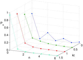
Figure 2: Photon number distribution for a GSS with $r_{0}=1$, $k=0.1$, $\nu_{0}=0$ and $\bar{n}_{B}=0$.

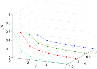
Figure 3: Photon number distribution for a GSS with $r_{0}=1$, $k=0.1$, $\nu_{0}=3$ and $\bar{n}_{B}=0$.

References

- (1) I. R. Senitzky, Phys. Rev. 95, 1115 (1954).
- (2) J. Plebanski, Phys. Rev. 101, 1825 (1956).
- (3) K. Husimi, Prog. Theor. Phys. 9, 381 (1953).
- (4) S. T. Epstein, Am. J. Phys. 27, 291 (1959).
- (5) S. L. Braunstein and P. van Loock, Rev. Mod. Phys. 77, 513 (2005).
- (6) C. H. Bennett et al, Phys. Rev. Lett. 70, 1895 (1993).
- (7) S. L. Braunstein and H. J. Kimble, Phys. Rev. A 61, 042302 (2000).
- (8) J. Fiuráŝek and N. J. Cerf, Phys. Rev. Lett. 93, 063601 (2004).
- (9) J. Wenger et al, Phys. Rev. A 70, 053812 (2004).
- (10) A. O. Caldeira and A. J. Leggett, Phys. Rev. Lett. 46, 211 (1981).
- (11) A. O. Caldeira and A. J. Leggett, Ann. Phys. (N.Y.) 149, 374 (1983).
- (12) R. Blume-Kohout and W. H. Zurek, Phys. Rev. A 68 032104 (2003).
- (13) E. G. Cavalcanti and M. D. Reid, Phys. Rev. Lett. 97, 170405 (2006).
- (14) J. W. Lee and D. L. Shepelyansky, Phys. Rev. E 71, 056202 (2005).
- (15) H. Han et al, J. Phys. B: At. Mol. Opt. Phys. 40, S209 (2007).
- (16) G. Y. Kryuchkyan and S. B. Manvelyan, Phys. Rev. A 68, 013823 (2003).
- (17) V. V. Dodonov, O. V. Man’ko and V. I. Man’ko, Phys. Rev. A 49, 2993 (1994).
- (18) J. Lages et al, Phys. Rev. E 72, 026225 (2005).
- (19) R. Rossi Jr., A. R. B. Magalhães and M. C. Nemes, Phys. Lett. A 356, 277 (2006).
- (20) P. Bianucci, J. P. Paz and M. Saraceno, Phys. Rev E 65, 046226 (2002).
- (21) K. M. F. Romero and M. C. Nemes, Physica A 325, 333 (2003).
- (22) K. Wódkiewicz et al, Phys. Rev A 35, 2567 (1987).
- (23) M. S. Kim, F. A. M. de Oliveira and P. L. Knight, Phys. Rev. A 40, 2494 (1989); F. A. M. de Oliveira et al, Phys. Rev. A 41, 2645 (1990).
- (24) V. Bužek, A. Vidiella-Barranco and P. L. Knight, Phys. Rev. A 45, 6570 (1992).
- (25) L. Gilles and P. L. Knight, Phys. Rev. A 48, 1582 (1993).
- (26) A. S. M. de Castro and V. V. Dodonov, Phys. Rev. A 73, 065801-1 (2006).
- (27) A. M. O. de Almeida, J. Phys. A.: Math. Gen. 36, 67 (2003).
- (28) Matteo G. A. Paris et al, Phys. Rev. A 68, 012314 (2003).
- (29) Serafini A., Paris M. G. A., Illuminati F. and De Siena S., J. Opt. B: Quantum Semiclass. Opt. 7, R19 (2005).
- (30) P. Marian and T. A. Marian, J. Phys. A: Math. Gen. 33, 3595 (2000).
- (31) M. Brune et al, Phys. Rev. A 45, 5193 (1992).
- (32) M. Brune et al, Phys. Rev. Lett. 65, 976 (1990).
- (33) S. P. Walborn et al, Nature 440, 1022 (London, 2006).
- (34) P. Sonnentag and F. Hasselbach, Phys. Rev. Lett. 98, 200402 (2007).
- (35) W. Wang, L. B. Fu, and X. X. Yi, Phys. Rev. A 75, 045601 (2007).
- (36) A. Serafini et al, Phys. Rev. A 69, 023318 (2004).
- (37) G. S. Agarwal, Phys. Rev. A 3, 828 (1971); for a review about Robertson-Schrödinger uncertainty principle see arXiv:quant-ph/9903100v2.
- (38) M. M. Nieto, Phys. Lett. A 229, 135 (1997).
- (39) P. Marian and T. A. Marian, Phys. Rev. A 47, 4474 (1993).
- (40) P. Marian and T. A. Marian, Phys. Rev. A 47, 4487 (1993).