Characterization of 2D fermionic insulating states

Abstract

Inspired by the duality picture between superconductivity (SC) and insulator in two spatial dimension (2D), we conjecture that the order parameter, suitable for characterizing 2D fermionic insulating state, is the disorder operator, usually known in the context of statistical transformation. Namely, the change of the phase of the disorder operator along a closed loop measures the particle density accommodating inside this loop. Thus, identifying this (doped) particle density with the dual counterpart of the magnetic induction in 2D SC, we can naturally introduce the disorder operator as the dual order parameter of 2D insulators. The disorder operator has a branch cut emitting from this “vortex” to the single infinitely far point. To test this conjecture against an arbitrary 2D lattice models, we have chosen this branch cut to be compatible with the periodic boundary condition and obtain a general form of its expectation value for non-interacting metal/insulator wavefunction, including gapped mean-field order wavefunction. Based on this expression, we observed analytically that it indeed vanishes for a wide class of band metals in the thermodynamic limit. On the other hand, it takes a finite value in insulating states, which is quantified by the localization length or the real-valued gauge invariant 2-from dubbed as the quantum metric tensor. When successively applied along a closed loop, our disorder operator plays role of twisting the boundary condition of a periodic system. We argue this point, by highlighting the Aharonov-Bohm phase associated with this non-local operator.

I Introduction

The high-$T_{\rm c}$ cuprates and the colossal magnetoresistive manganites, the two main realms in condensed matter physics, are both doped correlated insulators. As type II superconductors accommodate magnetic flux by allowing a spatially inhomogeneous distribution of the superconducting order parameter, such fermionic insulating states do not necessarily remain spatially uniform against doping. Indeed recent STM experiments have observed that a hole rich region in a doped Mott insulator such as Bi-2212 forms a nanoscale granular island on top of the insulating background lang . A similar kind of nanoscale electronic inhomogeneity was also found in Ca_2-xNa_xCuO₂Cl₂, where doped holes form a checkerboard pattern hana . On the other hand, extensive Lorentz optical microscopy measurements on doped (e.g., mixed valence) manganites have revealed that charge ordered and ferromagnetic metallic patches are phase-separated in such relatively large length scales as a few micrometer uehara . The question naturally arises as follows : Is there some universal classification of insulators in terms of their different types of behavior against doping? The other way around, if it exists, what kind of microscopic ingredients would determine these differences?

These experimental questions/observations as well as almost all the other experimental observables are directly accessible through the “local electronic polarization” $\vec{P}(\vec{r})$, which acquires finite mass only in dielectrics. Contrary to other observables, however, the local electronic polarizations cannot be uniquely determined by those vector fields which are divergence-free. Namely, using arbitrary analytic scalar functions $\theta(\vec{r})$, we can introduce those vector fields which have nothing to do with the local charge density $\rho(\vec{r})\equiv\vec{\nabla}\cdot\vec{P}(\vec{r})$;

$$\vec{P}^{\prime}(\vec{r}) = \vec{P}(\vec{r})+\times\vec{\nabla}\theta(\vec{r}),$$

$$\vec{\nabla}\cdot\vec{P}^{\prime}(\vec{r}) = \vec{\nabla}\cdot\vec{P}(\vec{r}).$$ (1)

Due to this arbitrariness, constructing effective theories of dielectrics in such a way that the local polarization becomes explicit has been one of the long-standing issues in condensed matter theories community, while widely demanded from experimental sides on a general ground.

The central idea of the duality picture is to regard this local electronic polarization as the “gauge field” which is intrinsic in matters and to treat its divergence-free part as the unphysical “gauge” degree of freedom. fisher ; balents1 ; balents2 ; tesanovic To be more specific, we suppose that there exist order parameters, implicit in a microscopic model, which are coupled with the local electronic polarization such that its condensation makes this “gauge fields” massive via the Higgs mechanism balents1 ; balents2 ; tesanovic . Accordingly, the “gauge” in eq.(1) and that of this order parameter $\eta(\vec{r})$ are specified in a set, as in superconductors;

$$\eta^{\prime}(\vec{r})=\eta(\vec{r})e^{i\theta(\vec{r})}.$$ (2)

where the vortex-free scalar function $\theta(\vec{r})$ should be identical to that in Eq. (1).

In this paper, observing this duality picture, we will introduce this complex-valued order parameter $\eta(\vec{r})$ explicitly in terms of original fermion (electron) operators. Then we calculate the expectation value of this order parameter with respect to some simple wavefunctions, so that we can argue that this order parameter has indeed a finite amplitude, i.e. condensed, only in fermionic insulators.

This paper is organized as follows : In Sec. II, we look further into the duality between superconductivity and insulator only to arrive at the conjecture that the appropriate order parameter for a 2D fermionic insulating state is the disorder operator (DOP) defined as eqs. (4,9). We then give a general expression to the expectation value of the DOP. In Sec. III, we will see that this expectation value indeed vanishes for band metals having various kinds of Fermi surface (F.S.) in the thermodynamic limit. In Sec. IV, we will consider the opposite limit, i.e., the case of a band insulator/gapped mean-field order state close to the atomic limit. Thereby, we observe that the expectation value of the DOP is in turn characterized by the localization length and thus remain finite. Then these two observations, i.e. those in sec. III and in sec. IV, lead us to extrapolate the behaviour of the DOP in general insulating states. Sec. V is devoted to the arguments on the relation between the DOP and “twisting boundary condition”, the latter known to give a definite criterion for insulating states in arbitrary spatial dimension kohn ; kudinov ; ivo ; scalapino . Sec. VI contains not only the brief summary (see Table. II) but also discussions on the behaviour of our DOP in the off-diagonal long ranged ordered states. We also mentioned there about the possible microscopic candidates of the counterpart of the magnetic penetration depth/coherence length (see Table. I) and the future possible progress. Some details of the calculation are left to the appendix.

II The disorder operator and the insulating order parameter

II.1 On duality between superconductivity and insulator

Let us denote the usual superconducting order parameter as $\Delta(\vec{r})=|\Delta(\vec{r})|e^{i\phi(\vec{r})}$. In this paper, we consider only two spatial dimension (2D), i.e. $\vec{r}=(x,y)$. If the magnetic penetration depth $\lambda$ is large enough compared with the coherence length $\xi$ (if $\kappa\equiv\lambda/\xi>1/\sqrt{2}$ in the conventional Ginzburg-Landau theory deG ), then the system shows a type II superconducting behavior, accommodating magnetic flux $b(\vec{r})$ pinned to vortices in the system. The amplitude of order parameter $|\Delta(\vec{r})|$ is spatially not uniform and can have zeros. Then its phase $\phi(\vec{r})$ acquires an ambiguity of integer multiples of $2\pi$ around its zeros. The holonomy of this phase around such a vortex is proportional to the number of magnetic flux pinned to this vortex, counted in units of the flux quantum $\Phi_{0}\equiv\hbar c/(2e)$. Let a flux penetrate a specific area $S$. Then, we have,

$$\Phi_{0}\oint_{\partial S}\nabla\phi(\vec{r})\cdot d\vec{l}=\int_{\vec{r}\in S}b(\vec{r})\ d^{2}r,$$ (3)

where $\nabla\equiv(\partial/\partial x,\partial/\partial y)$ and $\partial S$ is the boundary of this area $S$. We now invoke this relation to identify the dual quantity of $\Delta(\vec{r})$.

2D electronic insulator	2D superconductor
doping	applied magnetic field
doped particle density:	magnetic induction:
$\delta\rho(\vec{r})=\rho(\vec{r})-\bar{\rho}$	$b(\vec{r})$
“type I insulator (?)”	type I superconductor
“type II insulator (?)”	type II superconductor
?	penetration depth
?	coherence length
disorder operator:	order parameter:
$\eta(\vec{r})=|\eta(\vec{r})|e^{i\theta(\vec{r})}$	$\Delta(\vec{r})=|\Delta(\vec{r})|e^{i\phi(\vec{r})}$
$a_{\mu}(\vec{r})=\epsilon_{\mu\nu}P_{\nu}(\vec{r})=\nabla_{\mu}\theta(\vec{r})$	$A_{\mu}(\vec{r})=\nabla_{\mu}\phi(\vec{r})$
$\delta\rho(\vec{r})=\nabla\cdot\vec{P}=\nabla\times a$	$\delta b(\vec{r})=\nabla\times A$

Table 1: The duality between 2D insulator and superconductivity

In the duality relation between 2D superconductivity and 2D insulator, applying magnetic field in superconductors corresponds to doping in insulators lee1 (Table. I). Thus the doped particle density $\delta\rho(\vec{r})\equiv\rho(\vec{r})-\bar{\rho}$ corresponds to magnetic flux in superconductors. Physically speaking, $\delta\rho(\vec{r})$ is obtained from a local electronic polarization $\vec{P}(r)$; $\delta\rho(\vec{r})=\vec{\nabla}\cdot\vec{P}(r)$. Then introducing the “gauge field” $\vec{a}(\vec{r})$ such that ${a}_{\mu}(\vec{r})=\epsilon_{\mu\nu}P_{\nu}(\vec{r})$, we have only to find out a scalar function whose gradient is this “gauge field”, i.e. $\partial_{\mu}\theta(\vec{r})=a_{\mu}(\vec{r})$. Namely, we can identify this scalar function $\theta(\vec{r})$ as the phase part of the dual order parameter, i.e. counterpart of $\phi(\vec{r})$. We thus reach the conjecture that the disorder operator (DOP) $\tilde{\eta}(\vec{r})$ frad should play role of an insulating order parameter;

$$\tilde{\eta}(z)\equiv{\rm exp}\Big{[}\int_{z^{\prime}\neq z}d^{2}z^{\prime}\log(z^{\prime}-z)\left\{\rho(z^{\prime})-\bar{\rho}\right\}\Big{]}.$$ (4)

Here we have introduced a complex variable $z=x+iy$, and $d^{2}z$ should be understood to be $d^{2}z=d\bar{z}dz/(2i)$. Note that $\tilde{\eta}(\vec{r})$ is defined on a 2D infinite plane without any boundary condition. Using this explicit form, one can readily verify that eq. (4) indeed satisfies our leading principle,

$${1\over 2\pi}\oint_{\partial S}\nabla{\rm arg}\ \tilde{\eta}(\vec{r})\cdot d\vec{l}=\int_{\vec{r}\in S}\left\{\rho(\vec{r})-\bar{\rho}\right\}d^{2}\vec{r}.$$ (5)

This states that the winding number associated with the dual order parameter $\tilde{\eta}(\vec{r})$ is identical to the doped particle number inhabiting within $S$.

II.2 Disorder operator for a periodic lattice

Table. I shows the correspondence between 2D insulator and superconductivity. In the middle two empty seats are reserved for the unknown counterparts of the magnetic penetration depth and the coherence length in 2D insulator. If we push forward with this duality relation, our eventual goal might be to construct a Ginzburg-Landau theory for 2D (doped) insulating state in terms of this non-local operator, which unambiguously lets us complete this table quantitatively. As a first step toward this direction, we will demonstrate in the following sections that the expectation value of the DOP

1. indeed vanishes in various types of 2D band metals, i.e., the DOP is not condensed (see Sec. III), whereas

2. it remains finite in 2D band insulators, i.e., the DOP is condensed (see Sec. IV).

If one tries to make sure these statements, one might immediately notice that the DOP defined in eq. (4) in itself is incompatible with the periodic boundary condition (PBC) which we usually presume. The branch cut of logarithm in eq. (4) has only a single end point, while, mathematically speaking, it is impossible to embed such a branch cut into a torus.

A possible and the most plausible way out would be to replace $z^{\prime}-z$ in this logarithm by a doubly periodic function $\zeta(x^{\prime}-x,y^{\prime}-y)$, i.e. $\zeta(x,y+L)\equiv\zeta(x+L,y)\equiv\zeta(x,y)$, which reproduce $z^{\prime}-z$ when $|z^{\prime}-z|\ll L$,

$$\lim_{|z^{\prime}-z|/L\rightarrow 0}\zeta(x^{\prime}-x,y^{\prime}-y)\simeq z^{\prime}-z.$$ (6)

Here $L$ denotes the linear dimension of a system size. As the simplest function satisfying this requirement, we consider in this paper the following function,

$$\zeta(x^{\prime}-x,y^{\prime}-y)\equiv$$

$$\ \ -i\big{(}e^{i{2\pi\over L}(x^{\prime}-x-x_{0})}-1\big{)}+\big{(}e^{i{2\pi\over L}(y^{\prime}-y-y_{0})}-1\big{)}.$$ (7)

Apart from the continuum variables $z$ and $z^{\prime}$ used in eq. (4), $\vec{r}\equiv(x,y)$ and $\vec{r}^{\prime}\equiv(x^{\prime},y^{\prime})$ in eq. (7) are defined to take a discrete value, specifying lattice points in a particular lattice model. $(x_{0},y_{0})$ was then introduced, so as to avoid the logarithmic singularity when $\log\zeta$ are summed with respect to $\vec{r}^{\prime}$ over all lattice points (see eq. (9)). In a simple square lattice with its lattice constant “a”, we will take $(x_{0},y_{0})\equiv(\frac{\rm a}{2},\frac{\rm a}{2})$ (see Fig. 1).

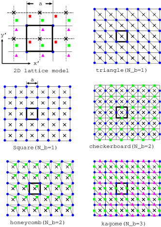
Figure 1: (color online) 2D lattice models. $(x,y)$ and $(x^{\prime},y^{\prime})$ specify a lattice point (filled circle mark). A unit cell is depicted as bold line in every figure and we use different colors (shapes) in order to distinguish $N_{b}$ number of inequivalent lattice points within it. Crossed mark represents a dual lattice site on which $(x+x_{0},y+y_{0})$ is located. (From top to down): Triangle and Square lattice with $N_{b}=1$, honeycomb and checkerboard lattice with $N_{b}=2$ and kagome lattice with $N_{b}=3$. Note that $(x+x_{0},y+y_{0})$ (crossed mark) never coincides with the original lattice sites on which a fermion operator is defined.

This function, i.e. eq. (7), in fact satisfies the requirement eq. (6). Namely, when $|z^{\prime}-z|\ll L$, it actually reads,

$$\zeta(x^{\prime}-x,y^{\prime}-y)\simeq{2\pi\over L}\{(x^{\prime}-x-x_{0})+i(y^{\prime}-y-y_{0})\}.$$

It is also a doubly periodic function. As a result, when seen as a continuous function of $(x^{\prime},y^{\prime})$, $\zeta(x^{\prime}-x,y^{\prime}-y)$ has two zeros:

$$(x^{\prime},y^{\prime})=(x+x_{0},y+y_{0}),\ \ \big{(}x+x_{0}+{L\over 4},y+y_{0}-{L\over 4}\big{)}.$$ (8)

The first zero corresponds to the original vortex introduced in eq. (4). The latter one turns out to be the antivortex, which was supposed to be located at the single infinitely far point in eq. (4). To be more specific, when $(x^{\prime},y^{\prime})$ moves around the former (latter) zero point anti-clockwise, then $\log\zeta$ picks up a phase $2\pi$ ($-2\pi$), as shown in Fig. 2. Accordingly, $\log\zeta$ has a branch cut running from the vortex to the antivortex as in Fig. 3. In general, the singularities must appear in pairs in a system obeying PBC. In order to study the DOP explicitly in non-interacting states and mean-field ordered states, it is necessary to write down a ground state wavefunction explicitly. Without PBC, we would not be able to do this. We thus conjecture in the remainder of the paper that the following operator with $\zeta$ defined in eq. (7) is the appropriate form of the disorder operator (DOP) compatible with PBC,

$$\eta(\vec{r})\equiv\exp\big{[}\sum_{x^{\prime},y^{\prime}}\log\zeta(x^{\prime}-x,y^{\prime}-y)\{\rho(\vec{r^{\prime}})-\bar{\rho}\}\big{]}.$$ (9)

Notice that the $z^{\prime}$-integral in eq. (4) avoids $z^{\prime}=z$, while the summation w.r.t. $\vec{r}^{\prime}\equiv(x^{\prime},y^{\prime})$ in eq. (9) is taken over entire lattice points without any restriction. As we mentioned above in the square lattice case with its lattice constant “a”, this simplification becomes possible, just because we have introduced $(x_{0},y_{0})=(\frac{\rm a}{2},\frac{\rm a}{2})$ so that $\log\zeta(n_{x}{\rm a},n_{y}{\rm a})$ is always finite for arbitrary integer $n_{x}$ and $n_{y}$. All 2D lattice models, however, can be also regarded as having a square unit cell (See Fig. 1). Then, we can always choose $(x_{0},y_{0})$ appropriately, such that the vortex and antivortex introduced in eq. (8) never coincide with any lattice points on which $\rho(\vec{r}^{\prime})$ is defined (see some examples shown in Fig. 1). Provided that $\log\zeta(\vec{r}^{\prime}-\vec{r})$ in eq. (9) takes finite value for an arbitrary lattice point $\vec{r}^{\prime}$, then the following arguments do not depend seriously on the specific choice of $(x_{0},y_{0})$.

Before giving the general expression to the expectation value of our DOP defined in eqs. (7,9), let us fix our ideogram of this paper now. Firstly, we always refer a lattice constant of a unit cell (square box depicted by bold line in Fig. 1) to “$\rm a$”. We take a number of this unit cell in an entire system to be $N\times N$ and thus the linear dimension of a system size is given by $L=N\rm a$. We call as $N_{b}$, the total number of Bloch bands/inequivalent sites within each unit cell, while total number of electrons which a ground state w.f. has is denoted by $N_{e}$. Then the average particle number per site $\bar{\rho}$ introduced in eq. (9) is given as follows,

$$\bar{\rho}\equiv\frac{N_{e}}{N_{b}\cdot N^{2}}.$$ (10)

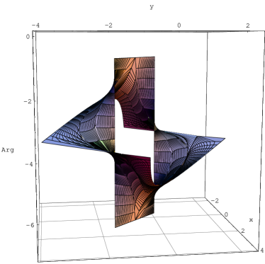
Figure 2: (color online) ${\rm Arg}{\rm log}[-i(e^{ix}-1)+(e^{iy}-1)]$ as a function of $x$ and $y$, where we only show the principle branch which ranges from $-\frac{\pi}{4}$ to $-\frac{9\pi}{4}$ in this picture and those below.

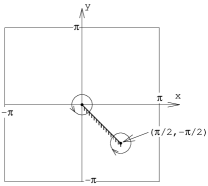
Figure 3: : A branch cut runs from the vortex $((x,y)=(0,0))$ to the anti-vortex $((x,y)=(\frac{\pi}{2},-\frac{\pi}{2}))$. ${\rm Arg}{\rm log}[-i(e^{ix}-1)+(e^{iy}-1)]$ takes $-\frac{\pi}{4}-$ in the shaded side of this branch cut, while takes $-\frac{9\pi}{4}+$ in the other side.

II.3 The general expression for expectation values of the disorder parameter

For a non-interacting system and arbitrary mean-field ordered state with $N_{e}$ fermions, a ground wavefunction is obtained just by filling the lowest $N_{e}$ one-body states which we name simply as $\alpha=1,2,\cdots,N_{e}$,

$$|{\rm GS}\rangle=c_{N_{e}}^{\dagger}c_{N_{e}-1}^{\dagger}\cdots c_{2}^{\dagger}c_{1}^{\dagger}|0\rangle.$$ (11)

Here $|0\rangle$ denotes the fermion-vacuum state. To evaluate our DOP for such a ground state, let us apply our DOP onto a creation or an annihilation operator. We define the matrix elements $\zeta[\alpha|\beta]$ as

$$\eta(\vec{r})c^{\dagger}_{\alpha}=\sum_{\beta}c_{\beta}^{\dagger}\zeta[\beta|\alpha]\eta(\vec{r}),$$ (12)

where $\alpha$ and $\beta$ specify a one-body electronic state. For sake of simplicity, we will make the $\vec{r}$ dependence of $\zeta[\alpha|\beta]$ implicit from now on. Since $\eta(\vec{r})$ is nonlocal, it does not commute even with creation and annihilation operators at different positions ($\vec{r^{\prime}}$). From the expression of $\eta(\vec{r})$ in eq. (9), we can readily see this,

$$\eta(\vec{r})c^{\dagger}(\vec{r^{\prime}})=\zeta(x^{\prime}-x,y^{\prime}-y)c^{\dagger}(\vec{r^{\prime}})\eta(\vec{r}).$$ (13)

On comparing this with eq. (12), we also see that $\zeta[\alpha|\beta]$ is diagonal in this real-space representation,

$$\zeta[\vec{r^{\prime}_{1}}|\vec{r^{\prime}_{2}}]=\delta(\vec{r^{\prime}_{1}}-\vec{r^{\prime}_{2}})\zeta(x^{\prime}_{1}-x,y^{\prime}_{1}-y).$$ (14)

In the momentum-space representation, however, $\alpha$ and $\beta$ is specified by the crystal momentum $\vec{k}$ and the band index $n=1,2,\cdots,N_{b}$. The creation operator of such a Bloch state is defined as follows,

$$c^{\dagger}_{n,\vec{k}}=\frac{1}{N}\sum_{\vec{r}}e^{-i\vec{k}\cdot\vec{r}}u_{n,\vec{k}}(\vec{r})c^{\dagger}_{\vec{r}},$$

where $u_{n,\vec{k}}(\vec{r})$ is the periodic part of the Bloch wavefunction. Then, substituting the above equation into eq. (13), we readily obtain the explicit matrix elements for $\zeta[\alpha|\beta]$ in this momentum representation,

$$\zeta[n,\vec{k}|n^{\prime},\vec{k^{\prime}}]=(i-1)\delta_{n,n^{\prime}}\delta_{\vec{k},\vec{k^{\prime}}}$$

$$-ie^{-i{2\pi\over L}(x+x_{0})}\Big{\langle}u_{n,(k_{x},k_{y})}\Big{|}u_{n^{\prime},(k_{x}+{2\pi\over L},k_{y})}\Big{\rangle}\delta_{k_{x},k^{\prime}_{x}-{2\pi\over L}}\delta_{k_{y},k^{\prime}_{y}}$$

$$+e^{-i{2\pi\over L}(y+y_{0})}\Big{\langle}u_{n,(k_{x},k_{y})}\Big{|}u_{n^{\prime},(k_{x},k_{y}+{2\pi\over L})}\Big{\rangle}\delta_{k_{x},k^{\prime}_{x}}\delta_{k_{y},k^{\prime}_{y}-{2\pi\over L}}.$$

(15)

where the inner product between $|u_{n,\vec{k}}\rangle$ represents an integral over the unit cell. These inner products are nothing but the gauge connections in $\vec{k}$ space. Note that, in this momentum representation, $\zeta[\alpha|\beta]$ is no longer diagonal. Instead, it takes a matrix form representing a $\vec{k}$-derivative or $\vec{k}$-covariant derivative. The above relations defined in eqs. (12)-(15) play a fundamental role in the reminder of the present paper.

II.3.1 The determinant formulae

Using the ground state wavefunction defined in eq. (11), let us formulate a general expression for its expectation value of the DOP,

$$\langle\eta(\vec{r})\rangle=\langle{\rm GS}|\eta(\vec{r})|{\rm GS}\rangle.$$ (16)

Noticing that for an arbitrary permutation of $N_{e}$ quantum numbers,

$${\rm sgn}(P)=$$

$$\langle 0|c_{1}c_{2}\cdots c_{N_{e}-1}c_{N_{e}}c_{P(N_{e})}^{\dagger}c_{P(N_{e}-1)}^{\dagger}\cdots c_{P(2)}^{\dagger}c_{P(1)}^{\dagger}|0\rangle,$$

one can readily verify,

$$\langle\eta(\vec{r})\rangle=\langle 0|\eta(\vec{r})|0\rangle\sum_{P}{\rm sgn}(P)$$

$$\times\zeta[P(N_{e})|N_{e}]\cdots\cdot\zeta[P(2)|2]\cdot\zeta[P(1)|1],$$ (17)

where $\langle 0|\eta(\vec{r})|0\rangle$ is a contribution from the uniform background $\bar{\rho}$. Leaving further analysis on $\langle 0|\eta(\vec{r})|0\rangle$ to the following subsection, let us for the moment consider eq. (17). The summation over $P$ should be taken for all the possible permutations of $N_{e}$ occupied states. Here, let us use eq. (15) as $\zeta[\alpha|\beta]$, bearing in mind a band metal/insulator. Then, in order to interpret the summation over $P$ as a determinant, we will arrange or rearrange every row and column in such a way that all the matrix elements $\zeta[\alpha|\beta]$ with $\alpha$ and $\beta$ being occupied Bloch states should be accommodated in the upper-left block of $\zeta$. Let us call this $N_{e}\times N_{e}$ submatrix as $\zeta^{\prime}$, i.e.,

$$\zeta=\left(\begin{array}[]{ccc|c}&&&\\ &\zeta^{\prime}&&*\\ &&&\\ \hline\cr&*&&*\\ \end{array}\right).$$

Then one can reinterpret eq. (17) as

$$\langle\eta(\vec{r})\rangle=\langle 0|\eta(\vec{r})|0\rangle\det\zeta^{\prime}.$$ (18)

Note that the final formula (18) itself is independent of the representation. In fact, when $|\rm GS\rangle$ were given by a Slater determinant composed by atomic orbitals totally localized in the real space, then we would use eq. (14) instead of eq. (15) as $\zeta$ and thus $\zeta^{\prime}$. However, a non-interacting band metal/insulator wavefunction (w.f.), including gapped mean-field w.f., is usually composed by extended Bloch w.f.. Thus, we will evaluate eq. (18), using mainly its momentum representation.

II.3.2 Contribution from the uniform background

Before ending this section, let us estimate the contribution from the uniform background, i.e. $\langle 0|\eta(\vec{r})|0\rangle$. From the definition of eq. (9), it reads,

$$\log\langle 0|\eta(\vec{r})|0\rangle=-\bar{\rho}\sum_{x^{\prime},y^{\prime}}\log\zeta(x^{\prime}-x,y^{\prime}-y).$$ (19)

By using the real-space representation of the matrix $\zeta$, i.e. eq. (14), it could be rewritten as

$$\log\langle 0|\eta(\vec{r})|0\rangle=-\bar{\rho}\log\det\zeta.$$

Recall that $\bar{\rho}$ is the average particle number per site; $\bar{\rho}\equiv\frac{N_{e}}{N_{b}N^{2}}$. Thus, in terms of the filling fraction per site $\nu\equiv\bar{\rho}$, $\langle 0|\eta(\vec{r})|0\rangle$ has the following compact form,

$$\langle 0|\eta(\vec{r})|0\rangle=\frac{1}{(\det\zeta)^{\nu}}.$$ (20)

We will use this expression in section. IV.

Apart from its compact re-expression, eq. (19) itself can be directly evaluated. Notice that we have only to estimate the amplitude of $\langle\eta(\vec{r})\rangle$, so as to check whether it (does not) vanishes in a metal (insulator) or not. Thus we will focus only on the real part of $\log\langle 0|\eta(\vec{r})|0\rangle$. At the leading order in the thermodynamic limit, i.e., at the order of ${\cal O}(L^{2})$, the summation with respect to (w.r.t.) $\vec{r^{\prime}}=(x^{\prime},y^{\prime})$ can be replaced by an integral (see appendix. A),

$$\log\langle 0|\eta(\vec{r})|0\rangle=-\frac{N_{e}}{4\pi^{2}}$$

$$\times\int_{0}^{2\pi}\int_{0}^{2\pi}d\theta_{x}d\theta_{y}\log\big{[}\left(e^{i\theta_{x}}+i\right)+\left(e^{i\theta_{y}}-1\right)\big{]}.$$

In term of complex variables, i.e. $z=e^{i\theta_{x}}$ and $z^{\prime}=e^{i\theta_{y}}$, this can be further written into the double contour integral around a unit circle,

$$\log\langle 0|\eta(\vec{r})|0\rangle$$

$$=-N_{e}\oint_{|z|=1}\frac{dz}{2\pi i}\oint_{|z^{\prime}|=1}\frac{dz^{\prime}}{2\pi i}{\log\big{[}z^{\prime}-z_{1}(z)\big{]}\over zz^{\prime}}.$$ (21)

In the r.h.s., we introduced $z_{1}(z)=-z+1-i$. When $|z_{1}(z)|>1$, the integrand of eq. (21), seen as a function of $z^{\prime}$, has no more poles other than $z^{\prime}=0$. Thus $z^{\prime}$ can be trivially integrated away. In other words, if we decompose the contour $|z|=1$ into $C_{>}$ and $C_{<}$, where $C_{>}=\{z|\ |z|=1,|z_{1}(z)|>1\}$ and $C_{<}=\{z|\ |z|=1,|z_{1}(z)|<1\}$, then one can evaluate the integral along $C_{>}$ in the following way;

$$\int_{C_{>}}\frac{dz}{2\pi i}\oint_{|z^{\prime}|=1}\frac{dz^{\prime}}{2\pi i}{\log\big{[}z^{\prime}-z_{1}(z)\big{]}\over zz^{\prime}}$$

$$=\int_{C_{>}}\frac{dz}{2\pi i}{\log\big{[}-z_{1}(z)\big{]}\over z}$$

$$={3\over 8}\log 2+{1\over\pi}\sum_{n=1}^{\infty}\frac{\sin(n\pi/4)}{n^{2}2^{n\over 2}}+i{9\over 16}\pi.$$

As for the contribution from $C_{<}$, one can safely verify that it is only pure imaginary.We also analyzed the contributions at the next leading order, i.e. at the order of ${\cal O}(L)$, which also turns out to be pure imaginary (see Appendix A). We thus obtain the following estimation for the uniform background contributions,

$$\log|\langle 0|\eta(\vec{r})|0\rangle|$$

$$=-\Big{[}{3\over 8}\log 2+{1\over\pi}\sum_{n=1}^{\infty}{\sin(n\pi/4)\over 2^{n\over 2}n^{2}}\Big{]}N_{e}+{\cal O}(1),$$ (22)

which can be evaluated as,

$$|\langle 0|\eta(\vec{r})|0\rangle|=\exp\big{[}-0.46N_{e}+{\cal O}(1)\big{]}.$$ (23)

The fact that $\log|\langle 0|\eta(\vec{r})|0\rangle|<-\frac{\ln 2}{2}N_{e}$ in the thermodynamic limit is one of the indispensable ingredients for our conjecture to make sense, the meaning of which will become clearer in the section. III.

III The band metal case

Our objective here is to demonstrate that the expectation value of the DOP indeed vanishes for the metallic state. By considering a single band metallic case, we will see explicitly how the presence of Fermi surface leads to the vanishing of the expectation value of the DOP. As a consequence, we are led to classify various types of Fermi surface (or Fermi sea) into three categories by their topology. In the multiband case, attentions should be paid to the role of the gauge connection in the momentum space.

III.1 Single band — topology of Fermi sea

Let us first consider the simplest case, i.e., that of a single-band metal with $N_{b}=1$. This case is almost trivial in the sense that the gauge connection in the $\vec{k}$ space does not appear. However, as we will see below, it is a good starting point for understanding why our DOP can possibly distinguish between a metal and an insulator. The matrix element (15) reduces in the single-band case to,

$$\zeta[\vec{n}|\vec{n^{\prime}}]=\sqrt{2}e^{i{3\over 4}\pi}\times$$

$$\ \Big{[}\delta_{\vec{n},\vec{n^{\prime}}}+\Gamma_{x}^{(0)}\delta_{n_{x},n_{x}^{\prime}-1}\delta_{n_{y},n^{\prime}_{y}}+\Gamma_{y}^{(0)}\delta_{n_{x},n^{\prime}_{x}}\delta_{n_{y},n^{\prime}_{y}-1}\Big{]},$$

(24)

where

$$\Gamma_{x}^{(0)} = {1\over\sqrt{2}}e^{i{3\over 4}\pi}e^{-i{2\pi\over L}(x+x_{0})},$$

$$\Gamma_{y}^{(0)} = {1\over\sqrt{2}}e^{-i{3\over 4}\pi}e^{-i{2\pi\over L}(y+y_{0})}.$$ (25)

Here we have parameterized crystal momenta as $n_{x(y)}=1,2,\cdots,N_{x(y)}$; $k_{x}=2\pi n_{x}/L,k_{y}=2\pi n_{y}/L$. Our Brillouin zone is thus doubly periodic, i.e., $n_{x}+N_{x}\equiv n_{x},n_{y}+N_{y}\equiv n_{y}$, forming a torus in $\vec{k}$-space. Although $N_{x}$ and $N_{y}$ are same, i.e. $N_{x}{\rm a}=N_{y}{\rm a}\equiv L$, we dare use different symbols, $N_{x}$ and $N_{y}$, only in this section just for clarity of the following explanations. The substantial simplification seen in eqs. (24) and (25), when compared with eq. (15), is clearly the disappearance of the gauge connections. In the single band case, the gauge connection associated with an overlap of two Bloch functions at different $\vec{k}$-points gives at most a trivial phase factor, thus erased by gauge transformations.

III.1.1 Two representations

In order to give an explicit matrix expression of $\zeta$ using eq. (24), let us introduce two representations. The question is how to order $N_{x}N_{y}$ indices, which we will perform in the following two steps:

1. (${k_{x},k_{y}}$)-representation: The most simple and convenient way to give an explicit expression to eq. (24) is to order all the $k_{x}$’s and $k_{y}$’s in the increasing order of $n_{x}$ and $n_{y}$. Since in our matrix representation for eq. (24), each row or column corresponds to a 2D lattice point $(n_{x},n_{y})$, we attribute, (i) the inner microscopic structure (inside a given block) to the index $n_{x}$ or $k_{x}$, and (ii) the outer block structure to the index $n_{y}$ or $k_{y}$. Then, the explicit matrix element of $\zeta$ is given by

   $$\zeta=\sqrt{2}e^{i{3\over 4}\pi}\times$$

   $$\hskip 8.5359pt\Big{[}I^{(N_{x}N_{y})}+\Gamma^{(0)}_{x}\Sigma_{x}^{(N_{x},N_{y})}+\Gamma^{(0)}_{y}\Sigma_{Y}^{(N_{x},N_{y})}\Big{]},$$

   (26)

   with $I^{(N)}$ being an $N\times N$ identity matrix,

   $$\Sigma_{x}^{(N_{x},N_{y})}=\left(\begin{array}[]{c|c|c|c|c}S_{1}^{(N_{x})}&O^{(N_{x})}&\cdots&\cdots&O^{(N_{x})}\\ \hline\cr O^{(N_{x})}&S_{1}^{(N_{x})}&\ddots&&\vdots\\ \hline\cr\vdots&\ddots&\ddots&\ddots&\vdots\\ \hline\cr\vdots&&\ddots&S_{1}^{(N_{x})}&O^{(N_{x})}\\ \hline\cr O^{(N_{x})}&\cdots&\cdots&O^{(N_{x})}&S_{1}^{(N_{x})}\end{array}\right),$$ (32)

   and

   $$\Sigma_{Y}^{(N_{x},N_{y})}=\left(\begin{array}[]{c|c|c|c|c|c}O^{(N_{x})}&I^{(N_{x})}&O^{(N_{x})}&\cdots&\cdots&O^{(N_{x})}\\ \hline\cr\vdots&O^{(N_{x})}&I^{(N_{x})}&\ddots&&\vdots\\ \hline\cr\vdots&&\ddots&\ddots&\ddots&\vdots\\ \hline\cr\vdots&&&\ddots&I^{(N_{x})}&O^{(N_{x})}\\ \hline\cr O^{(N_{x})}&&&&O^{(N_{x})}&I^{(N_{x})}\\ \hline\cr I^{(N_{x})}&O^{(N_{x})}&\cdots&\cdots&\cdots&O^{(N_{x})}\end{array}\right).$$ (39)

   $S_{1}^{(N)}$ is an $N\times N$ shift matrix defined as

   $$S^{(N)}_{1}=\left(\begin{array}[]{cccccc}0&1&0&\cdots&\cdots&0\\ \vdots&0&1&\ddots&&\vdots\\ \vdots&&\ddots&\ddots&\ddots&\vdots\\ \vdots&&&\ddots&1&0\\ 0&&&&0&1\\ 1&0&\cdots&\cdots&\cdots&0\end{array}\right).$$ (40)

   $\Sigma_{x}^{(N_{x},N_{y})}$ and $\Sigma_{Y}^{(N_{x},N_{y})}$ can be thus written symbolically as

   $$\Sigma_{x}^{(N_{x},N_{y})} = S_{1}^{(N_{x})}\bigotimes I^{(N_{y})},$$

   $$\Sigma_{Y}^{(N_{x},N_{y})} = I^{(N_{x})}\bigotimes S_{1}^{(N_{y})}.$$

   Different subscripts, $x$ and $Y$, are used so as to recall that these two matrices contain a nontrivial structure at micro and MACRO-scopic levels.

2. Filtered-$(k_{x},k_{y})$-representation: In eq. (18), we gave an expression of the expectation value of the DOP in terms of the determinant of $N_{e}\times N_{e}$ matrix $\zeta^{\prime}$. This matrix, $\zeta^{\prime}$, is a submatrix of $\zeta$ and composed of the matrix elements between occupied states. In order to construct $\zeta^{\prime}$, we filter each state by whether it is occupied or not, i.e., we rearrange the order of the states in such a way that occupied states are in the first $N_{e}$ rows and columns in the upper-left block of $\zeta$, by keeping the ordering w.r.t. $n_{x}$ and $n_{y}$. We call this representation as $f$-representation in the following. It is apparent that these two representations are related to each other by an orthogonal transformation.

III.1.2 Three types of Fermi sea

The evaluation of the determinant (18) would be trivial if all the ($N,1$)-components $S^{(N)}_{1}$ were filtered in $\zeta^{\prime}$. Then the matrix $\zeta^{\prime}$ becomes an upper-triangular matrix and its determinant becomes just the product of the diagonal elements. The question is whether this ($N,1$)-element survives in $\zeta^{\prime}$ in the $f$-representation. This is actually dependent on the topology of Fermi sea, which we would like to discuss now.

Let us first consider a Fermi sea of trivial topology, which has null winding number along both $k_{x}$ and $k_{y}$-axes (Fig. 4(a)). Recall that a $(N_{x},1)$-element of $S_{1}^{(N_{x})}$ in $\Sigma_{x}^{(N_{x},N_{y})}$ is the matrix element between $(N_{x},n_{y})$ and $(1,n_{y})$. Both of these $\vec{k}$-points are, however, filtered away in the $f$-representation for an arbitrary $n_{y}$, since our Fermi sea does not wind the torus along the $k_{x}$-axis at all. Thus any $(N_{x},1)$-elements of $S_{1}^{(N_{x})}$ in $\Sigma_{x}^{(N_{x},N_{y})}$ do not survive in $\zeta^{\prime}$. In a same way, one can easily see that $(N_{y},1)$-block of $\Sigma_{Y}^{(N_{x},N_{y})}$ is totally filtered away and does not enter into $\zeta^{\prime}$ either. As a result, $\zeta^{\prime}$ becomes an upper-triangular matrix, whose determinant is identically 1 up to a trivial prefactor,

$$\det\zeta^{\prime}=2^{N_{e}\over 2}e^{i{3\pi\over 4}N_{e}}.$$ (41)

In order to see whether the DOP vanishes or not, we have to compare this value with $|\langle 0|\eta(\vec{r})|0\rangle|$, i.e., eqs. (22) and (23). We readily obtain,

$$\log|\langle\eta(\vec{r})\rangle| \simeq \Big{[}{1\over 8}\log 2-{1\over\pi}\sum_{n=1}^{\infty}\frac{\sin(n\pi/4)}{n^{2}2^{n\over 2}}\Big{]}N_{e}$$ (42)

$$\simeq -0.11N_{e}.$$

Thus we have verified that the DOP vanishes in the thermodynamic limit for the metallic state of trivial Fermi sea topology.

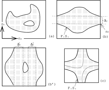
Figure 4: (a) type-O Fermi surface with uneven boundary and annulus. (b) Type-A or B Fermi surface. The strip, which is enclosed by the two dashed straight line, winds the torus along $k_{x}$-direction. (b’) Another type-A or B Fermi surface. The presence of annulus inside the Fermi sea does not change the type of the Fermi surface. Namely, we have only to replace $\Delta_{y}$ in eq. (44) by $\Delta^{1}_{x}+\Delta^{2}_{x}$. (c) Type-AB F.S. with a loop which winds around the torus along $k_{x}$ and $k_{y}$-direction.

Let us now consider a less trivial case, i.e., the case of such a Fermi sea as depicted in Figs. 4(b) and (b’). The Fermi sea winds the torus either along $k_{x}$ or $k_{y}$-axes. Suppose that the Fermi sea has a filled strip which round the torus along the $k_{x}$ direction as in Fig. 4 (b). Then the strip is specified by $k_{y}={2\pi\over L}n_{y}$, where $n_{y}$ takes such values as $n_{y}=n_{0},n_{0}+1,\cdots,n_{0}+\Delta_{y}-1$ on the strip. The width of the strip is therefore determined by $\Delta_{y}$ to be $2\pi\Delta_{y}/L$ (see in Fig. 4(b)).

The Fermi surface topology along the $k_{y}$-axis is, however, still trivial. Thus $(N_{y},1)$-block of $\Sigma_{Y}^{(N_{x},N_{y})}$ is totally filtered. Then the matrix $\zeta^{\prime}$ turns out to be block upper-triangle in the $f$-representation. The determinant of $\zeta^{\prime}$, therefore, can be factorized into the product of the determinants of diagonal blocks specified by $n_{y}$. Furthermore, for any $k_{y}$ or $n_{y}$ which is out of the strip, the “topology” along the $k_{x}$-axis is trivial. Namely, if one considers a row specified by $n_{y}$ in the $(k_{x},k_{y})$-plane such that $n_{y}<n_{0}$ or $n_{y}>n_{0}+\Delta-1$, this row does not wind the torus along the $k_{x}$-axis. Thus all the submatrices (diagonal blocks) in $\zeta^{\prime}$ which are specified by either $n_{y}<n_{0}$ or $n_{y}>n_{0}+\Delta_{y}-1$ are always the upper-triangular matrix, whose determinant is identically 1 up to a trivial factor. Then the calculation of $\det\zeta^{\prime}$ reduces to those of $\Delta_{y}$ diagonal submatrices corresponding to the strip. They all have the form $\sqrt{2}e^{i{3\over 4}\pi}(I^{(N_{x})}+\Gamma^{(0)}_{x}S^{(N_{x})}_{1})$. Since $\det[I^{(N_{x})}+\Gamma^{(0)}_{x}S_{1}^{(N_{x})}]$ can be readily calculated as $1+(-1)^{N_{x}-1}(\Gamma^{(0)}_{x})^{N_{x}}$, one finally finds,

$$\det\zeta^{\prime}=2^{N_{e}\over 2}e^{i{3\pi\over 4}N_{e}}\Big{[}1+(-1)^{N_{x}-1}\big{(}\Gamma^{(0)}_{x}\big{)}^{N_{x}}\Big{]}^{\Delta_{y}}.$$ (43)

Observing

$$1+(-1)^{N_{x}-1}\big{(}\Gamma_{x}\big{)}^{N_{x}}<1+2^{-{N_{x}\over 2}}<1+{1\over N_{x}}$$

for $N_{x}\gg 1$, we can readily overestimate $|\det\zeta^{\prime}|$ as follows,

$$|\det\zeta^{\prime}|<2^{N_{e}\over 2}e^{\Delta_{y}\over N_{x}}.$$ (44)

In the end, we takes the thermodynamic limit, keeping the ratio $\Delta_{y}/N_{x}$ fixed (to be smaller than 1). Then $e^{\Delta_{y}\over N_{x}}$ gives a correction of at most ${\cal O}(1)$ in the exponential of the expectation value of the DOP, $|\langle\eta(\vec{r})\rangle|\simeq\exp\big{[}-0.11N_{e}+{\cal O}(1)\big{]}$. Thereby the correction is obviously irrelevant and the DOP indeed vanishes again in the thermodynamic limit.

Finally it is also possible that the Fermi sea envelopes the torus along both $k_{x}$ and $k_{y}$-axes as depicted in Fig. 4(c), where the Fermi sea has four pockets at each corner of the Brillouin zone (therefore still metallic). In this case the submatrix $\zeta^{\prime}$ is no longer block upper-triangle. It is not impossible to write down formally $\det\zeta^{\prime}$, but its estimation needs some numerical analysis. We have verified by a simple numerical analysis with substantial system size that expectation value of the DOP for a band metal having this class of Fermi surface exhibits an exponential decay w.r.t. the system size.

III.2 Multiple band case without filled bands

When there are more than a single band, the situation becomes suddenly complicated, because of (i) the presence of gauge connection, and (ii) the inter-band matrix elements associated with gauge connection. However, we can still give a quantitative argument by simply adding $N_{b}-1$ empty bands to the single-band case studied above. Namely, in such a situation, we have only to calculate the determinant of the matrix elements in the lowest band $n=1$. In other words, only intra-band ($n=1$) gauge connection appears in our analysis. Because of this simplification, we can still use exceptionally the single-band equation (26), but $\Gamma_{\mu}^{(0)}$ in eq.(26) should be replaced by the following $N_{x}N_{y}$ by $N_{x}N_{y}$ diagonal matrices,

$$\Gamma_{\mu}^{(0)}\rightarrow$$

$$\ \ \ \Gamma^{(N_{x},N_{y})}_{\mu}[\vec{n}|\vec{n}^{\prime}]\equiv\Gamma_{\mu}^{(0)}\cdot\langle u_{1,\vec{k}}|u_{1,\vec{k}+\vec{e}_{\mu}}\rangle\delta_{\vec{n},\vec{n}^{\prime}},$$ (45)

Here the unit vectors in the $\vec{k}$ space were introduced for convenience; $\vec{e}_{x}\equiv\frac{2\pi}{L}(1,0)$ and $\vec{e}_{y}\equiv\frac{2\pi}{L}(0,1)$.

Let us first consider a Fermi sea of trivial topology as depicted in Fig. 4(a). As we have seen in the previous subsection, the submatrix $\zeta^{\prime}$, spanned by the occupied states, becomes trivially an upper-triangular matrix in this case. Thus, there is clearly no room for $\Gamma^{(N_{x},N_{y})}_{\mu}$ to play a role. The determinant again reduce to 1 up to a trivial prefactor $2^{N_{e}\over 2}e^{i\frac{3\pi}{4}N_{e}}$.

The case of second topology such as Figs. 4(b) is probably more interesting. The arguments are totally parallel until $\det\zeta^{\prime}$ is factorized into $\Delta_{y}$ diagonal block matrices, which are now not completely same. They still have a similar form as $\sqrt{2}e^{i{3\over 4}\pi}(I^{(N_{x})}+\Gamma^{(0)}_{x}S^{(N_{x})}_{1})$. But, due to the replacement of eq.(45), these $\Delta_{y}$ diagonal block matrices are also modified as,

$$I^{(N_{x})}+\Gamma^{(0)}_{x}S^{(N_{x})}_{1}\rightarrow I^{(N_{x})}+\Gamma^{(N_{x})}_{x}(n_{y})\cdot S^{(N_{x})}_{1},$$ (46)

where $n_{y}$ takes such values as $n_{y}=n_{0},n_{0}+1,\cdots,n_{0}+\Delta_{y}-1$ on the strip. The $N_{x}\times N_{x}$ diagonal matrices $\Gamma^{(N_{x})}_{x}(n_{y})$ in the r.h.s. are defined as $\Gamma^{(N_{x})}_{x}(n_{y})[n_{x}|{n_{x}}^{\prime}]\equiv\Gamma^{(N_{x},N_{y})}_{x}[n_{x},n_{y}|{n_{x}}^{\prime},n_{y}]$. As the number of the permutation associated with the determinants of both matrices in eq. (46) is same, the determinant of the r.h.s. is also readily calculated;

$$\det[I^{(N_{x})}+\Gamma_{x}^{(N_{x})}(n_{y})\cdot S_{1}^{(N_{x})}]$$

$$=1+(-1)^{N_{x}-1}\left(\Gamma_{x}^{(0)}\right)^{N_{x}}\prod_{n_{x}=1}^{N_{x}}\big{\langle}u_{1,\vec{k}}\big{|}u_{1,\vec{k}+\vec{e}_{x}}\big{\rangle}.$$ (47)

Hence, we have

$$\det\zeta^{\prime}=2^{N_{e}\over 2}e^{i{3\pi\over 4}N_{e}}\times$$

$$\prod_{n_{y}=n_{0}}^{n_{0}+\Delta_{y}-1}\Big{\{}1+(-1)^{N_{x}-1}\left(\Gamma_{x}^{(0)}\right)^{N_{x}}\prod_{n_{x}=1}^{N_{x}}\big{\langle}u_{1,\vec{k}}\big{|}u_{1,\vec{k}+\vec{e}_{x}}\big{\rangle}\Big{\}},$$

where $\prod_{n_{x}=1}^{N_{x}}$ is a product along a closed loop parallel to the $k_{x}$-axis. One might dub this loop as $C(k_{y})$ in the sense that it is specified only by $k_{y}$. The product of gauge connection along this closed loop can be rewritten in terms of the integral of the abelian gauge field, $\langle u_{1,\vec{k}}|\partial_{k_{x}}u_{1,\vec{k}}\rangle$, w.r.t. $k_{x}$,

$$\prod_{n_{x}=1}^{N_{x}}\big{\langle}u_{1,\vec{k}}\big{|}u_{1,\vec{k}+\vec{e}_{x}}\big{\rangle}$$

$$=\ \exp\Big{[}\int_{C(k_{y})}\langle u_{1,\vec{k}}|\partial_{k_{x}}u_{1,\vec{k}}\rangle\ dk_{x}+{\cal O}\big{(}\frac{1}{N_{x}}\big{)}\Big{]}.$$ (48)

Since this gauge field is pure imaginary, the amplitude of the r.h.s. is always unity in the thermodynamic limit. We thus conclude that the estimation in the previous subsection, i.e., eq. (44), is still unchanged even in the presence of the abelian gauge connections. The DOP still vanishes as $\sim\exp[-0.11N_{e}+{\cal O}(1)]$.

In the case of the multiple band with finite number of completely filled bands, we have no direct analytic proof that the expectation value of our DOP vanishes in metal. This is because all the filled bands form a torus and the situation associated with these filled bands is essentially same as the F.S. depicted in Fig. 4(c). In those situations, we need to check our conjecture with a help of some numerics in future. Summary of this section is listed in the table. II of the section. VI.

IV Band Insulator/Mean-field ordered state

Observing the results in Sec. III that the DOP vanishes in the metallic case whenever it could be evaluated so far, we will complete our another task in this section. Our purpose here is to verify that the expectation value of the DOP indeed remains finite in band insulators and gapped mean-field ordered states. In the crystal momentum space, the lowest $N_{v}$ bands are completely filled. The remaining $N_{b}-N_{v}$ bands are totally empty. Then, on filtering away these empty bands, the expectation value of the DOP reads,

$$\langle\eta\rangle=\langle{\rm GS}|\eta|{\rm GS}\rangle={\det\zeta^{\prime}\over(\det\zeta)^{\nu}}.$$

Here we used eq. (20) as the background contributions $\langle 0|\zeta|0\rangle$. $\zeta^{\prime}$ is the upper left part of $\zeta$ in the $f$-representation, i.e. spanned only by the filled $N_{v}$ bands. Unlike the F.S. depicted in Figs. 4(a), (b) and (b’), it was totally impossible, even in $N_{v}=1$ case, to factorize this determinant into the product of diagonal elements or diagonal blocks. Additional complications appear, when one considers a more general case, i.e. $1<N_{v}<N_{b}$. The gauge connections between different filled bands make it much larger the number of the permutation associated with the determinant of $\zeta^{\prime}$.

In order to resolve these difficulties, we first focus on the most strongly localized limit, i.e. the atomic limit. We define this limit, such that a Hamiltonian is decoupled into a local Hamiltonian defined for each unit cell. These local Hamiltonians commute with one another. Thus eigenstates of a full Hamiltonian are given by eigenstates of each local Hamiltonian, which we call as localized atomic orbitals. Bloch bands, which is totally flat in $\vec{k}$-space in this limit, can be then obtained, on Fourier-transforming these localized atomic orbitals. The periodic part of the Bloch function $|u_{n,\vec{k}}\rangle$ thus obtained has no $\vec{k}$-dependence in this limit.

Starting from this atomic limit, we will expand $\langle\eta\rangle$ in powers of the number of $k$-derivatives of this periodic part. This treatment is verified, provided that our system is close to the atomic limit. We will perform this expansion up to the second order and observe that $|\langle\eta\rangle|$ in the insulating state is characterized by the quantum metric tensor defined in eq. (52) (See also eq. (62)). When integrated over the crystal momentum, this gauge invariant 2-form is directly linked to the physical quantity called as the localization length $\xi$ (eqs. (53,54)). Then, we discuss that our DOP remains finite, as far as this localization length is finite. Before developing this perturbation expansion specifically, we give a brief reminder to the relation between localization length and metric tensor, including their physical meanings.

IV.1 brief review – arbitrariness of Wannier function, its spread functional and quantum metric tensor

The relation between the quantum metric tensor in the $\vec{k}$ space and localization length were discovered in the process of constructing a gauge invariant localized Wannier function. Taking Fourier transformation of Bloch w.f., one can usually introduce a spatially “localized” single particle w.f. called as Wannier functions,

$$\langle\vec{r}|\vec{R},n\rangle=\frac{1}{N^{2}}\sum_{\vec{k}\in{\rm Bz}}e^{i\vec{k}\cdot(\vec{r}-\vec{R})}u_{n,\vec{k}}(\vec{r}).$$ (49)

However, this single particle w.f. is clearly not invariant under the $U(1)$ gauge transformation, $\tilde{u}_{n,\vec{k}}(\vec{r})=e^{i\phi_{n\vec{k}}}u_{n,\vec{k}}(\vec{r})$, while any physical quantities should be. In the case of a composite set of bands, say $N_{v}$ filled bands, the corresponding gauge transformation is generalized into $SU(N_{v})$ gauge transformations. In either case, shapes of Wannier functions depend on a particular gauge fixing and are unphysical by themselves.

Marzari and Vanderbilt introduced a unique set of gauge independent Wannier functions, by minimizing the spread functional associated with this single particle w.f. marzari ,

$$\Omega=\sum_{n=1}^{N_{v}}\Big{[}\langle\vec{0},n|\vec{r}^{2}|\vec{0},n\rangle-\left(\langle\vec{0},n|\vec{r}|\vec{0},n\rangle\right)^{2}\Big{]},$$ (50)

where measuring $\Omega$ at $\vec{R}=\vec{0}$ does not lose any generality. Namely, by optimizing the $SU(N_{v})$ gauge degrees of freedom such that this spread functional $\Omega$ is minimized, we could defined the maximally localized set of Wannier functions $\{|\vec{R},n\rangle\}$. This set of Wannier functions is by definition gauge invariant. They further prove in ref. marzari, that, when optimized, this spread functional becomes

$$\Omega_{I}=\sum_{n=1}^{N_{v}}\Big{[}\langle\vec{0},n|\vec{r}^{2}|\vec{0},n\rangle-\sum_{\vec{R},m}\big{|}\langle\vec{R},m|\vec{r}|\vec{0},n\rangle\big{|}^{2}\Big{]}.$$ (51)

The localization length $\xi$ is introduced as this minimized spread; $\xi^{2}\equiv\Omega_{I}$. Using the identity,

$$\langle\vec{R},n|r_{\mu}r_{\nu}\cdots|\vec{0},m\rangle=$$

$$\ \frac{1}{N^{2}}\sum_{\vec{k}\in{\rm Bz}}e^{i\vec{k}\cdot\vec{R}}\langle u_{n,\vec{k}}|(i\nabla_{k_{\mu}})(i\nabla_{k_{\nu}})\cdots|u_{m,\vec{k}}\rangle,$$

one can then express this length $\xi$ in terms of the following “metric tensor” defined as marzari ; ivo ; resta2 ,

$$g_{\mu\nu}(\vec{k})\equiv\sum_{n=1}^{N_{v}}{\rm Re}\ \Big{[}\big{\langle}\partial_{k_{\mu}}u_{n,\vec{k}}\big{|}\partial_{k_{\nu}}u_{n,\vec{k}}\big{\rangle}$$

$$\ \ -\ \sum_{n^{\prime}=1}^{N_{v}}\big{\langle}\partial_{k_{\mu}}u_{n,\vec{k}}\big{|}u_{n^{\prime},\vec{k}}\big{\rangle}\big{\langle}u_{n^{\prime},\vec{k}}\big{|}\partial_{k_{\nu}}u_{n,\vec{k}}\big{\rangle}\Big{]}.$$ (52)

Namely, we have

$$\xi^{2}=\sum_{\mu}\xi_{\mu}^{2},\ \ \ \xi_{\mu}^{2}=\frac{1}{N^{2}}\sum_{\vec{k}\in{\rm Bz}}g_{\mu\mu}(\vec{k}).$$ (53)

As is clear from this definition, $\xi$ vanishes in the atomic limit, where $|u_{n,\vec{k}}\rangle$ has no $\vec{k}$-dependence.

The tensor quantity $g_{\mu\nu}$ is dubbed as the quantum metric tensor, in the sense that it measures the minimal distance between two sets of $N_{v}$ eigenbasis $\{|u_{n,\vec{k}}\rangle\}$ and $\{|u_{n,\vec{k}+d\vec{k}}\rangle\}$. In fact, when optimizing the $SU(N_{v})$ gauge degree of freedom such that $\sum_{n=1}^{N_{v}}|\langle u_{n,\vec{k}}|u_{n,\vec{k}+d\vec{k}}\rangle|$ is minimized, this quantum distance is indeed specified by $g_{\mu\nu}(\vec{k})dk_{\mu}dk_{\nu}$ anandan .

The localization length thus introduced can be generalized into the following correlation function of macroscopic electronic polarizations, measured w.r.t. the ground state many-body w.f. $|{\rm GS}\rangle$ ivo ,

$$\xi^{2}_{\mu}=\frac{1}{N_{e}}\big{\langle}{\rm GS}\big{|}\big{(}\hat{X}_{\mu}-\bar{X}_{\mu}\big{)}^{2}\big{|}{\rm GS}\big{\rangle},$$ (54)

where $\hat{X}_{\mu}\equiv\sum_{j=1}^{N_{e}}\hat{x}_{j,\mu}$ denotes the total electron’s position operator. This correlation function is infinite when a system has a Drude weight or peak, while remains finite without any Drude weight ivo . Thus, $\xi$ is also finite (infinite) in insulators (metal).

IV.2 Disorder operator from the viewpoint of localization length

We see below that the expectation value of the DOP in insulating states is simply related to the localization length, as given in eq. (63). To be specific, starting with the atomic limit, we expand $\log\langle\eta\rangle$ in powers of $\partial_{\vec{k}}|u_{n\vec{k}}\rangle$. The zero-th order, which corresponds to the atomic limit, gives a constant contribution. At the first order, one finds a correction due to the gauge field. However, this is pure imaginary, and irrelevant to the amplitude of $\langle\eta\rangle$. The first relevant contribution to $|\langle\eta\rangle|$ appears at the second order, which will be interpreted, with the help of eqs. (52,53), as the square of localization length. Then, eq. (63) in combination with eq. (54) tells us that the DOP remains finite in insulators, as far as this perturbation expansion is valid. Since the localization length diverges in metals, a naïve extrapolation of our second order analytic expression is also consistent with our previous observations found in the metallic case.

IV.2.1 The zeroth order – atomic limit

In the atomic limit (AL), where $|u_{n,\vec{k}}\rangle$ has no $\vec{k}$-dependence, the gauge connection becomes a trivial matrix, i.e. $\langle u_{n,\vec{k}}|u_{n^{\prime},\vec{k}^{\prime}}\rangle=\delta_{n,n^{\prime}}$. Then the matrix $\zeta$ takes the following decoupled structure in the momentum representation,

$$\zeta_{\rm AL}[n,\vec{k}|n^{\prime},\vec{k}^{\prime}]=\delta_{n,n^{\prime}}\otimes\zeta_{\rm SB}[\vec{k}|\vec{k^{\prime}}].$$

From eq. (15), $\zeta_{\rm SB}[\vec{k}|\vec{k^{\prime}}]$ is simply given as follows,

$$\zeta_{\rm SB}[\vec{k}|\vec{k^{\prime}}]=\big{(}\gamma_{x}\delta_{\vec{k}+\vec{e}_{x},\vec{k}^{\prime}}+i\delta_{\vec{k},\vec{k}^{\prime}}\big{)}+\big{(}\gamma_{y}\delta_{\vec{k}+\vec{e}_{y},\vec{k}^{\prime}}-\delta_{\vec{k},\vec{k}^{\prime}}\big{)},$$

where $\gamma_{\mu}$ is $\sqrt{2}e^{i\frac{3\pi}{4}}\Gamma^{(0)}_{\mu}$. This $N^{2}$ by $N^{2}$ matrix is diagonalized by the Fourier transformation, where the unit cell index: $\vec{R}=(n_{x}{\rm a},n_{y}{\rm a})$, specifies its eigenvector, i.e. $e^{i\vec{k}\cdot\vec{R}}$. The corresponding eigenvalue of $\zeta_{\rm SB}$ reads,

$$\lambda({\vec{R}})=\big{(}\gamma_{x}e^{i\vec{e}_{x}\cdot\vec{R}}+i\big{)}+\big{(}\gamma_{y}e^{i\vec{e}_{y}\cdot\vec{R}}-1\big{)}.$$ (55)

As the band index and momentum index are decoupled in $\zeta_{\rm AL}$, we can easily filter unfilled bands so as to obtain $\log\det\zeta^{\prime}_{\rm AL}={\rm Tr}\log\zeta^{\prime}_{\rm AL}$. In other words, we have only to sum $\log\lambda(\vec{R})$ w.r.t. the unit cell index $\vec{R}$ and multiply the number of filled atomic orbital within each unit cell;

$$\log\det\zeta_{\rm AL}^{\prime}=N_{v}\sum_{n_{x},n_{y}=1}^{N}\log\lambda({\vec{R}}).$$

Notice that $\lambda(\vec{R})$ in eq. (55) is basically same as the original $\zeta(\vec{R}-\vec{r})$ defined in eq. (7). Thus we can relate the r.h.s. with $\det\zeta$ used in eq. (20),

$$\log\det\zeta_{\rm AL}^{\prime}=\frac{N_{v}}{N_{b}}\cdot N_{b}\sum_{\vec{R}}\log\lambda({\vec{R}})=\nu\cdot\log\det\zeta,$$

where $\nu=\frac{N_{e}}{N_{b}N^{2}}$. This tells us a rather trivial fact that our DOP becomes unit in this atomic limit, $\langle\eta\rangle_{\rm AL}={\det\zeta_{\rm AL}^{\prime}\over(\det\zeta)^{\nu}}=1$ note .

IV.2.2 First and second orders

We now introduce weak transfer integrals between the localized atomic orbitals, taking into account weak $\vec{k}$-dependences of $|u_{n,\vec{k}}\rangle$ perturbatively. Namely, we develop a perturbative expansion in powers of the number of its $\vec{k}$-derivative. To concretize the perturbative evaluation of $\det\zeta^{\prime}/(\det\zeta)^{\nu}$, let us consider its logarithm, i.e. $\log\det\zeta^{\prime}={\rm Tr}\log\zeta^{\prime}$, and decompose $\zeta^{\prime}$ as $\zeta^{\prime}=\zeta^{\prime}_{\rm AL}+\Delta\zeta^{\prime}$. $\Delta\zeta^{\prime}$ describes the deviation from the atomic limit, in which the information of weak delocalizations are encoded through the “gauge field” $\hat{\cal A}_{\mu}(\vec{k})$,

$${\cal A}_{\mu}^{[n|n^{\prime}]}(\vec{k}) \equiv \big{\langle}u_{n,\vec{k}}\ \bigl{|}\ u_{n^{\prime},\vec{k}+\vec{e}_{\mu}}\big{\rangle}-\delta_{n,n^{\prime}}$$ (56)

$$= \frac{2\pi}{L}\big{\langle}u_{n,\vec{k}}\big{|}\partial_{k_{\mu}}u_{n^{\prime},\vec{k}}\big{\rangle}+$$

$$\frac{1}{2}\big{(}\frac{2\pi}{L}\big{)}^{2}\big{\langle}u_{n,\vec{k}}\big{|}\partial^{2}_{k_{\mu}}u_{n^{\prime},\vec{k}}\big{\rangle}+{\cal O}\big{(}\partial^{3}_{\vec{k}}\big{)}.$$

$\Delta\zeta^{\prime}$ is written in terms of this “gauge field” as

$$\Delta\zeta^{\prime}[n,\vec{k}|n^{\prime},\vec{k}^{\prime}]=\sum_{\mu=x,y}\gamma_{\mu}\delta_{\vec{k}+\vec{e}_{\mu},\vec{k}^{\prime}}{\cal A}_{\mu}^{[n|n^{\prime}]}(\vec{k}),$$

where $n$ and $n^{\prime}$ are restricted within filled bands. Observing that $\Delta\zeta^{\prime}$ contains at least the first order of $\partial_{\vec{k}}|u_{n,\vec{k}}\rangle$, we first expand ${\rm Tr}\log(\zeta^{\prime}_{\rm AL}+\Delta\zeta^{\prime})$ w.r.t. $\Delta\zeta^{\prime}$,

$${\rm Tr}\log(\zeta^{\prime}_{\rm AL}+\Delta\zeta^{\prime})=\log{\rm det}\big{[}\zeta^{\prime}_{\rm AL}\big{]}+{\rm Tr}\big{[}{\zeta^{\prime}_{\rm AL}}^{-1}\Delta\zeta^{\prime}\big{]}$$

$$\hskip 34.14322pt-\ \frac{1}{2}{\rm Tr}\big{[}{\zeta^{\prime}_{\rm AL}}^{-1}\Delta\zeta^{\prime}{\zeta^{\prime}_{\rm AL}}^{-1}\Delta\zeta^{\prime}\big{]}+{\cal O}\big{(}\partial^{3}_{\vec{k}}\big{)}.$$ (57)

As was shown above, its zero-th order term is cancelled by the contribution from the uniform background $\langle 0|\eta|0\rangle=1/(\det\zeta)^{\nu}$, when exponentiated. On the other hand, using the inverse of $\zeta^{\prime}_{\rm AL}$,

$${\zeta^{\prime}_{\rm AL}}^{-1}[n,\vec{k}|n^{\prime},\vec{k^{\prime}}]=\delta_{n,n^{\prime}}\frac{1}{N^{2}}\sum_{\vec{R}}e^{i(\vec{k}-\vec{k}^{\prime})\cdot\vec{R}}\lambda(\vec{R})^{-1},$$

the 1st order term w.r.t. the “gauge field” $\hat{\cal A}_{\mu}$ is given as follows,

$${\rm Tr}\big{[}{\zeta^{\prime}_{\rm AL}}^{-1}\Delta\zeta^{\prime}\big{]}=\sum_{\mu=x,y}\sum_{\vec{k}\in{\rm Bz}}\sum_{n=1}^{N_{v}}{\cal A}_{\mu}^{[n|n]}(\vec{k})\times$$

$$\hskip 48.36958pt{1\over N^{2}}\sum_{\vec{R}}\frac{\gamma_{\mu}e^{i\vec{e}_{\mu}\cdot\vec{R}}}{\big{(}\gamma_{x}e^{i\vec{e}_{x}\cdot\vec{R}}+i\big{)}+\big{(}\gamma_{y}e^{i\vec{e}_{y}\cdot\vec{R}}-1\big{)}}.$$

The coefficient of $\hat{\cal A}_{\mu}$ can be further evaluated by the following double counter integral,

$$\frac{1}{N^{2}}\sum_{\vec{R}}\frac{\gamma_{\mu}e^{i\vec{e}_{\mu}\cdot\vec{R}}}{(\gamma_{x}e^{i\vec{e}_{x}\cdot\vec{R}}+i)+(\gamma_{y}e^{i\vec{e}_{y}\cdot\vec{R}}-1)}=$$

$$\int\!\!\!\int_{[0,2\pi]\times[0,2\pi]}\frac{e^{i\theta_{\mu}}}{e^{i\theta_{x}}+i+e^{i\theta_{y}}-1}\ \frac{d\theta_{x}d\theta_{y}}{4\pi^{2}}+{\cal O}\big{(}\frac{1}{L^{2}}\big{)},$$

where the complex variable $e^{i\theta_{\mu}}\equiv\gamma_{\mu}e^{i\vec{e}_{\mu}\cdot\vec{R}}$ was introduced. Notice that the integrand in the r.h.s. can be simply replaced by $-i\partial_{\theta_{\mu}}\{\log[e^{i\theta_{x}}+i+e^{i\theta_{y}}-1]\}$,

$$\int\!\!\!\int_{[0,2\pi]\times[0,2\pi]}\frac{e^{i\theta_{\mu}}}{e^{i\theta_{x}}+i+e^{i\theta_{y}}-1}\ \frac{d\theta_{x}d\theta_{y}}{4\pi^{2}}$$

$$=-\frac{i}{4\pi^{2}}\int_{0}^{2\pi}d\theta_{\bar{\mu}}\int_{0}^{2\pi}d\theta_{\mu}\partial_{\theta_{\mu}}\big{\{}\ln[e^{i\theta_{x}}+i+e^{i\theta_{y}}-1]\big{\}},$$

where $\bar{\mu}$ denotes the other coordinate than $\mu$ e.g. $\bar{x}\equiv y$. As was clear from Figs. 2,3,10, $\log[e^{i\theta_{x}}+i+e^{i\theta_{y}}-1]$ has a branch cut, which runs from $(-\pi/2,0)$ to $(0,-\pi/2)$ in the $\theta_{x}$-$\theta_{y}$ plane. Thus a surface term associated with the $\theta_{\mu}$-integral in the r.h.s. gives $2\pi i$, when its integral path crosses this branch cut. Then, irrespective of a specific choice of the principle branch, this double counter integral is always estimated to be $1/4$ (see Fig. 10 in the case of $\mu=x$);

$$\int\!\!\!\int_{[0,2\pi]\times[0,2\pi]}\frac{e^{i\theta_{\mu}}}{e^{i\theta_{x}}+i+e^{i\theta_{y}}-1}\ \frac{d\theta_{x}d\theta_{y}}{4\pi^{2}}$$

$$=-\frac{i}{4\pi^{2}}\int_{-\frac{\pi}{2}}^{0}d\theta_{\bar{\mu}}\cdot 2\pi i=\frac{1}{4}.$$ (58)

Using this coefficient, the 1st order term w.r.t. $\hat{\cal A}_{\mu}$ in eq. (57) then becomes as follows,

$${\rm Tr}[\ \zeta^{-1}_{\rm AL}\Delta\zeta]=\frac{1}{4}\sum_{\mu=x,y}\int_{-\frac{\pi}{\rm a}}^{\frac{\pi}{\rm a}}\int_{-\frac{\pi}{\rm a}}^{\frac{\pi}{\rm a}}dk_{x}dk_{y}\sum_{n=1}^{N_{v}}\Big{\{}\frac{N\rm a}{2\pi}\big{\langle}u_{n}\big{|}\partial_{k_{\mu}}u_{n}\big{\rangle}+\frac{1}{2}\big{\langle}u_{n}\big{|}\partial^{2}_{k_{\mu}}u_{n}\big{\rangle}\Big{\}}+{\cal O}\Big{(}\frac{1}{L},\partial^{3}_{\vec{k}}\Big{)},$$ (59)

where we further expanded the “gauge field” $\hat{\cal A}_{\mu}$ up to ${\cal O}(\partial^{2}_{\vec{k}})$, according to eq. (56).

Note that the integrand in eq.(59) contains the 2nd order derivative of $|u_{n}\rangle$ w.r.t. the crystal momentum, i.e. $\langle u_{n}|\partial^{2}_{k_{\mu}}u_{n}\rangle$. As we mentioned above, this 2nd order derivative term is more important than the 1st order one, i.e. $\langle u_{n}|\partial_{k_{\mu}}u_{n}\rangle$, when it comes to the amplitude of $\langle\eta\rangle$. Namely, the latter one is clearly pure imaginary, while the real part of the 2nd order derivative term, i.e. $\langle\partial_{k_{\mu}}u_{n}|\partial_{k_{\mu}}u_{n}\rangle$, constitutes a metric tensor in combination with ${\rm Tr}[\ ({\zeta^{\prime}_{\rm AL}}^{-1}\Delta\zeta^{\prime})^{2}]$, which we will see below.

${\rm Tr}[\ ({\zeta^{\prime}_{\rm AL}}^{-1}\Delta\zeta^{\prime})^{2}]$ has a relatively complicated form:

$${\rm Tr}[{\zeta^{\prime}_{\rm AL}}^{-1}\Delta\zeta^{\prime}{\zeta^{\prime}_{\rm AL}}^{-1}\Delta\zeta^{\prime}]=$$

$$\sum_{\mu,\nu}\sum_{\vec{k},\vec{k}^{\prime}}\sum_{n=1}^{N_{v}}\sum_{n^{\prime}=1}^{N_{v}}{\cal A}^{[n|n^{\prime}]}_{\mu}(\vec{k}){\cal A}^{[n^{\prime}|n]}_{\nu}(\vec{k}^{\prime})$$

$$\times\frac{1}{N^{2}}\sum_{\vec{R}}\frac{\gamma_{\mu}e^{i(\vec{k}+\vec{e}_{\mu}-\vec{k}^{\prime})\cdot\vec{R}}}{\gamma_{x}e^{i\vec{e}_{x}\cdot\vec{R}}+i+\gamma_{y}e^{i\vec{e}_{y}\cdot\vec{R}}-1}$$

$$\times\frac{1}{N^{2}}\sum_{\vec{R}^{\prime}}\frac{\gamma_{\nu}e^{i(\vec{k}^{\prime}+\vec{e}_{\nu}-\vec{k})\cdot\vec{R}^{\prime}}}{\gamma_{x}e^{i\vec{e}_{x}\cdot\vec{R}^{\prime}}+i+\gamma_{y}e^{i\vec{e}_{y}\cdot\vec{R}^{\prime}}-1}.$$ (60)

However, this can be still simplified substantially, by noticing that only the leading term is relevant to our ${\cal O}(\partial^{2}_{\vec{k}})$-estimations, in the expansion of $\hat{\cal A}_{\nu}(\vec{k}^{\prime})$ around $\vec{k}^{\prime}=\vec{k}$, i.e. $\hat{\cal A}_{\nu}(\vec{k}^{\prime})=\hat{\cal A}_{\nu}(\vec{k})+(\vec{k}^{\prime}-\vec{k})_{\lambda}\cdot\partial_{k_{\lambda}}\hat{\cal A}_{\nu}(\vec{k})+\cdots.$ Namely, higher order terms in this expansion lead to at least the third order $\vec{k}$-derivative of $|u_{n,\vec{k}}\rangle$, when substituted into Eq. (60). Thus, we fairly replace $\hat{\cal A}_{\nu}(\vec{k^{\prime}})$ in Eq. (60) by $\hat{\cal A}_{\nu}(\vec{k})$. This replacement enables us to sum over $\vec{k}^{\prime}$, which brings about a factor $N^{2}\delta_{\vec{R},\vec{R}^{\prime}}$. Accordingly, as far as the ${\cal O}(\partial^{2}_{\vec{k}})$-estimation is concerned, eq. (60) reduces to the following simple form;

$${\rm Tr}\big{[}{\zeta^{\prime}_{\rm AL}}^{-1}\Delta\zeta^{\prime}{\zeta^{\prime}_{\rm AL}}^{-1}\Delta\zeta^{\prime}]=$$

$$\ \ \sum_{\mu,\nu}\sum_{\vec{k}}\sum_{n=1}^{N_{v}}\sum_{n^{\prime}=1}^{N_{v}}{\cal A}^{[n|n^{\prime}]}_{\mu}(\vec{k}){\cal A}^{[n^{\prime}|n]}_{\nu}(\vec{k})$$

$$\ \ \times\frac{1}{N^{2}}\sum_{\vec{R}}\frac{\gamma_{\mu}\gamma_{\nu}e^{i(\vec{e}_{\mu}+\vec{e}_{\nu})\cdot\vec{R}}}{\big{(}\gamma_{x}e^{i\vec{e}_{x}\cdot\vec{R}}+i+\gamma_{y}e^{i\vec{e}_{y}\cdot\vec{R}}-1\big{)}^{2}}+{\cal O}\big{(}\partial^{3}_{\vec{k}}\big{)}.$$

Observing this simplification, one can readily see that the coefficients of $\hat{\cal A}_{\mu}\cdot\hat{\cal A}_{\nu}$ become diagonal w.r.t. $\mu$ and $\nu$. Evaluate the summation w.r.t. $\vec{R}$ in the r.h.s., in term of the double counter integral w.r.t. $\theta_{x}$ and $\theta_{y}$ introduced above,

$$\frac{1}{N^{2}}\sum_{\vec{R}}\frac{\gamma_{\mu}\gamma_{\nu}e^{i(\vec{e}_{\mu}+\vec{e}_{\nu})\cdot\vec{R}}}{\big{(}\gamma_{x}\ e^{i\vec{e}_{x}\cdot\vec{R}}+i+\gamma_{y}\ e^{i\vec{e}_{y}\cdot\vec{R}}-1\big{)}^{2}}=$$

$$\int\!\!\!\int_{[0,2\pi]\times[0,2\pi]}e^{i\theta_{\mu}}\ i\frac{\partial}{\partial\theta_{\nu}}\big{(}\frac{1}{\ e^{i\theta_{x}}+i+e^{i\theta_{y}}-1}\big{)}\ \frac{d\theta_{x}d\theta_{y}}{4\pi^{2}}.$$

Then, integrated by part w.r.t. $\theta_{\nu}$, the r.h.s. clearly vanishes when $\mu\neq\nu$, while becomes identical to the l.h.s. of eq. (58) when $\mu=\nu$. Thus, they are indeed diagonal w.r.t. $\mu$ and $\nu$;

$$\frac{1}{N^{2}}\sum_{\vec{R}}\frac{\gamma_{\mu}\gamma_{\nu}e^{i(\vec{e}_{\mu}+\vec{e}_{\nu})\cdot\vec{R}}}{\big{(}\gamma_{x}\ e^{i\vec{e}_{x}\cdot\vec{R}}+i+\gamma_{y}\ e^{i\vec{e}_{y}\cdot\vec{R}}-1\big{)}^{2}}=\frac{1}{4}\delta_{\mu\nu}+\big{(}\frac{1}{L^{2}}\big{)}.$$

Using this, the 2nd order term w.r.t. $\hat{\cal A}_{\mu}$ is then estimated up to the accuracy of ${\cal O}(\partial^{2}_{\vec{k}})$,

$${\rm Tr}\big{[}\ {\zeta^{\prime}_{\rm AL}}^{-1}\Delta\zeta^{\prime}{\zeta^{\prime}_{\rm AL}}^{-1}\Delta\zeta^{\prime}]=-\ \frac{1}{4}\sum_{\mu=x,y}\sum_{n,n^{\prime}=1}^{N_{v}}$$

$$\times\int_{\frac{-\pi}{\rm a}}^{\frac{\pi}{\rm a}}\int_{\frac{-\pi}{\rm a}}^{\frac{\pi}{\rm a}}dk_{x}dk_{y}\big{|}\big{\langle}u_{n^{\prime}}\big{|}\partial_{k_{\mu}}u_{n}\big{\rangle}\big{|}^{2}+{\cal O}\big{(}\frac{1}{L},\partial^{3}_{\vec{k}}\big{)}.$$ (61)

Notice the coincidence between the factor $\frac{1}{4}$ of eq. (61) and that of eq. (59). This coincidence actually helps us to combine these two contributions so as to obtain the gauge invariant ${\cal O}(\partial^{2}_{\vec{k}})$-estimation for the amplitude of our DOP,

$$\ln|\langle\eta(\vec{r})\rangle|=-\frac{1}{8}\sum_{\mu=x,y}\int_{-\frac{\pi}{\rm a}}^{\frac{\pi}{\rm a}}\int_{-\frac{\pi}{\rm a}}^{\frac{\pi}{\rm a}}dk_{x}dk_{y}\times$$

$$\sum_{n=1}^{N_{v}}\Big{\{}\big{\langle}\partial_{k_{\mu}}u_{n}\big{|}\partial_{k_{\mu}}u_{n}\big{\rangle}-\sum_{n^{\prime}=1}^{N_{v}}\big{|}\big{\langle}u_{n^{\prime}}\big{|}\partial_{k_{\mu}}u_{n}\big{\rangle}\big{|}^{2}\Big{\}}.$$ (62)

Namely, the integrand is nothing but diagonal components of the quantum metric tensor defined in eq. (52). Using the localization length defined in eq. (53), we then rewrite this as follows,

$$|\langle\eta(\vec{r})\rangle|=\exp\big{[}-{\pi^{2}\over 2}\bar{\xi}^{2}\big{]}.$$ (63)

where $\bar{\xi}$ is the dimensionless localization length, i.e. $\bar{\xi}\equiv\frac{\xi}{\rm a}$. As we have already mentioned, the localization length is infinite (finite) when the system has a (no) Drude weight or peak ivo . Thus, eq. (63) indicates that our DOP indeed remains finite in band insulators/gapped mean-field ordered states.

This 2nd order estimation was, however, derived perturbatively w.r.t. the $\vec{k}$-derivative of the periodic part of the Bloch w.f.. Thus eq. (63) obviously holds true only for small $\bar{\xi}$ region closed to the atomic limit. However, this simplest relation gives a key to extrapolate our analyses in this section to the metallic case studied previously. Namely, starting from the atomic limit where the localization length is zero, we slowly turn on the transfer integral between atomic orbitals so as to increase $\bar{\xi}$. Eq. (63) indicates that increase of the localization length reduces the amplitude of our DOP. We could further increase the inter-atomic transfer such that the band gap eventually collapses and a Fermi surface appears. Although this situation is clearly beyond the validity of our expansion, the indication of eq. (63) is still consistent with our analyses in Sec. III. Namely, as the localization length diverges on the appearance of Fermi surface, eq. (63) means that the DOP should indeed vanish in such a metallic case.

V “Twisting” boundary conditions and the disorder operator

To help readers to obtain a transparent interpretation of the disorder operator, we will attempt in this section to clarify the similarity between our DOP approach and other recipes or criteria for probing insulating behaviors. A standard recipe is to investigate system’s response against “twisting” the boundary conditions kohn ; scalapino . The twisted boundary condition along the $\mu$-direction requires the many-body wavefunction $\Phi(\vec{r}_{1},\cdots,\vec{r}_{N_{e}})$ obeys

$$\Phi(\cdots,\vec{r}_{i}+L\ \vec{e}_{\mu},\cdots)=e^{i\phi}\Phi(\cdots,\vec{r}_{i},\cdots)$$ (64)

for arbitrary $i$, where real-valued $\phi$ can be non-zero modulo $2\pi$. With the ground state wavefunction obeying this twisted boundary condition, one can take the 2nd order derivative of its eigen-energy with respect to $\phi$. This quantity estimated at a finite system size becomes the Drude weight, when considered in the thermodynamic limit, i.e. $L,N_{e}\rightarrow\infty$.

Notice that this twisted boundary condition can be transcribed into the magnetic flux $\phi$ inserted into those Hamiltonians obeying the periodic boundary condition kohn ; scalapino . Namely, as far as its eigen-energy is concerned, we may as well consider the Hamiltonian defined on the torus having its genus pierced by the non-zero flux $\phi$. In the following, highlighting the Aharonov-Bohm phase created by the DOP, we will argue that applying the DOP “successively” along a certain path $E$ on the 2D plane is also equivalent to inserting $2\pi\times{\rm(integer)}$ flux into a system;

$$\prod_{\vec{r}\in{\rm path}\ E}\eta(\vec{r})\simeq e^{i\frac{2\pi}{L}\times m\sum_{\vec{r}^{\prime}}r^{\prime}_{\mu}\rho(\vec{r}^{\prime})}.$$ (65)

Here the r.h.s. is the unitary transformation, sometimes dubbed as “twist operator”, which introduces $2\pi\times m$ flux through the genus associated with the $\mu$-direction.

V.1 flux insertion and the disorder operator

To determine the path $E$ in eq. (65) and also $\mu$ in its r.h.s., let us recall the detailed analytic properties of the DOP first,

$$\eta(\vec{r}) = \exp\big{[}\sum_{x^{\prime},y^{\prime}}\log\zeta(\vec{r}^{\prime}-\vec{r})\{\rho(\vec{r^{\prime}})-\bar{\rho}\}\big{]}$$

$$\zeta(\vec{r^{\prime}}-\vec{r}) = -i\big{(}e^{i{2\pi\over L}(x^{\prime}-x)}-1\big{)}+\big{(}e^{i{2\pi\over L}(y^{\prime}-y)}-1\big{)}.$$

Here we have already chosen as $x_{0}=y_{0}=0$, for the sake of simplicity. Its essential feature is actually the existence of vortex-antivortex pair. The vortex is located at $(x^{\prime},y^{\prime})=(x,y)$, whereas the antivortex at $(x^{\prime},y^{\prime})=(x+L/4,y-L/4)$. A branch cut runs, e.g., on the straight line, $x^{\prime}+y^{\prime}=x+y$, and connects the vortex with the antivortex, encoding the $U(1)$ phase holonomy associated with those singularities. In fact, one can see from Eq. (13) that ${\rm Im}\log\zeta(\vec{r^{\prime}}-\vec{r})$ corresponds to the “AB phase” which an electron at $\vec{r}^{\prime}$ subjected under $\eta(\vec{r})$ acquires while traveling on the 2D plane. For example, under the influence of the DOP, an electron winding the vortex anti-clockwise acquires $2\pi$ AB phase. Based on this observation, we naturally come up with the idea of representing the analytic structure of $\eta(\vec{r})$, i.e. a pairwise form of the vortex and anti-vortex, by introducing a flux tube piercing the system at these singularities.

In order to materialize this point, imagine that our 2D periodic system, forming a torus, resides in an 3D space. Our flux tube also lives in this space and intersects with the 2D plane at these two singular points. Namely, on the $(x^{\prime},y^{\prime})$-plane, it appears outside the torus at $(x,y)$, i.e., at the vortex, and after traveling above our 2D plane, it disappears inside the torus at the antivortex $(x+L/4,x-L/4)$, forming eventually a closed loop behind the system (see Fig. 5(a). The viewpoint of Fig. 5 is located clearly outside the torus.)

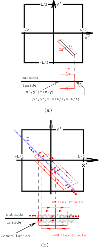
Figure 5: (Color online) (a) A quantized ($2\pi$) flux tube associated with the disorder operator (DOP) $\eta(\vec{r})$ is shown as a red(thin) arrows on the $(x^{\prime},y^{\prime})$-plane. Corresponding to the phase inconsistency of $\log\zeta(\vec{r^{\prime}}-\vec{r})$, the flux tube appears outside the torus at $(x,y)$, i.e., at the vortex, and after traveling above the branch cut, it disappears inside the torus at the antivortex, $(x+L/4,x-L/4)$, forming a loop. (b) The path $E$ is a straight blue (dotted) line along which a series of flux tubes associated with the DOP $\eta(\vec{r})$ is considered. Flux tubes associated with $\eta(\vec{r})$ at each lattice site $\vec{r}$ on $E$ are superposed. In this summation over $\vec{r}$ on $E$, cancellations between flux tubes heading outside and inside the system occur on the 2D plane (shadowed region). As a result, those flux which penetrate the system completely disappear, leaving two bundles of flux tubes above and beneath the system in parallel with $E$ (See also Fig. 6(a)).

Let us now consider a successive application of $\eta(\vec{r})$ on the straight line $E$ parallel to $x+y={\rm constant}$, i.e. $\prod_{\vec{r}\in E}\eta(\vec{r})$. In the language of this flux tube, this corresponds to a superposition of the flux tubes which are shifted by one lattice site (diagonally along $E$) between one another (Fig. 5(b)). When these tubes are superposed, cancellations between vortices and antivortices occur in the vicinity of 2D plane, and the singularities on the plane totally disappear. As a result, we are left with two decoupled vortex lines: one running above, the other beneath the system along $E$ (Fig. 6(a)). These are a bundle of $N/4$ quantized ($2\pi$) flux tubes; $N/4$, because of $N$ sites (operators) along $E$ and each operator having a branch cut of length, equal to 1/4 of the whole trajectory of $E$ ($=\sqrt{2}L$).

These two vortex lines can be deformed freely outside or inside the torus without intersecting the torus. Namely, as for an electron living in the 2D plane (torus), this freedom itself corresponds to a trivial $U(1)$ gauge degrees of freedom. Using this freedom, one can readily see that these two decoupled vortex lines indeed compose a pair of “knotted” rings, consisting of a “Hopf link” (Fig. 6(b)). In other words, we have

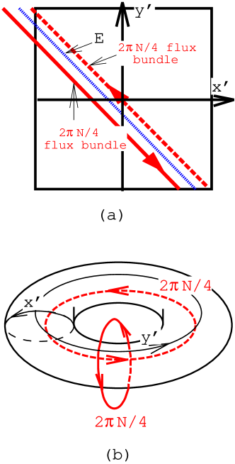
Figure 6: (Color online) (a) Two flux bundles and the periodic 2D flat surface ($=$ our system). The red(solid) line represents a bundle of $N/4$ quantized flux tubes which flows above ($\leftrightarrow$ outside the torus) and in parallel with our 2D plane. The red(broken) line is the other bundle which flows beneath ($\leftrightarrow$ inside the torus) and in parallel with the plane. (b) Two flux bundles and the torus ($=$ our system). The former pierces the handle of the torus encircled by the $y^{\prime}$-axis, whereas the latter penetrates the interior of the torus wound by the $x^{\prime}$-axis.

$$\prod_{\vec{r}\in E}\eta(\vec{r})\simeq e^{i\frac{2\pi}{L}\times\frac{N}{4}\sum_{\vec{r}^{\prime}}(x^{\prime}+y^{\prime})\rho(\vec{r}^{\prime})}.$$ (66)

This formula is almost correct, but there are two minor imperfections. First, the two sides of eq. (66) cannot be completely identical, since our DOP is not unitary, whereas the r.h.s. is clearly unitary. We, therefore, slightly soften our statement in such a way that the unitary part of $\prod_{\vec{r}\in E}\eta(\vec{r})$ is equivalent to the r.h.s. in Eq. (66). Secondly, since we freely deformed two vortex lines without intersecting our 2D plane, we can not fix in eq. (66) a trivial $U(1)$ phase factor $e^{i\varphi_{E}}$ with a real-valued continuous periodic function $\varphi_{E}(\vec{r}^{\prime})$;

1. $\partial_{x}\partial_{y}\varphi_{E}=\partial_{y}\partial_{x}\varphi_{E}$,

2. $\varphi_{E}(x^{\prime}+L,y^{\prime})=\varphi_{E}(x^{\prime},y^{\prime}+L)=\varphi_{E}(x^{\prime},y^{\prime})$.

Then, to the best of accuracy, our claim can be reformulated, in the language of the phase part of the DOP and twist operators, as

$$\sum_{\vec{r}}^{E}{\rm Im}\log\zeta(\vec{r}^{\prime}-\vec{r})={2\pi\over L}\times{N\over 4}(x^{\prime}+y^{\prime})+\varphi_{E}(\vec{r^{\prime}}).$$ (67)

V.2 Direct calculation of phase holonomy

Eq. (67) elucidated by the heuristic argument can be directly verified, on taking lattice constant “${\rm a}$” infinitesimally small with $N{\rm a}\equiv L$ fixed. In this continuum limit, the summation over $\vec{r}=(x,y)$ along $E$ is replaced by the integral w.r.t. $l=\frac{x-y}{\sqrt{2}}$ with fixed $\bar{l}\equiv\frac{x+y}{\sqrt{2}}$,

$$\frac{4}{N}\sum_{\vec{r}}^{E}{\rm Im}\log\zeta(\vec{r}^{\prime}-\vec{r}) = \frac{4}{\sqrt{2}L}\int_{-\frac{L}{\sqrt{2}}}^{\frac{L}{\sqrt{2}}}dl\ {\rm Im}\log\zeta(\vec{r}^{\prime}-\vec{r})$$ (68)

$$\equiv F(x^{\prime},y^{\prime};\bar{l}),$$

which is a function of $\bar{l}^{\prime}-\bar{l}$ in general. Then, by integrating $\partial_{r^{\prime}_{\mu}}F$ along the $r^{\prime}_{\mu}$-direction over $[-\frac{L}{2},\frac{L}{2}]$, we can directly calculate the AB phase which an electron acquires each time it travels around the periodic system along $r^{\prime}_{\mu}$-direction. Let us see this phase holonomy, taking $r^{\prime}_{\mu}$ to be $x^{\prime}$ first,

$$\int_{-\frac{L}{2}}^{\frac{L}{2}}\frac{\partial F}{\partial x^{\prime}_{\mu}}dx^{\prime}=$$

$$\frac{4}{\sqrt{2}L}\int_{-\frac{L}{\sqrt{2}}}^{\frac{L}{\sqrt{2}}}dl\ \int_{\frac{-L}{2}}^{\frac{L}{2}}\frac{\partial}{\partial x^{\prime}}\Big{\{}{\rm Im}\log\zeta(\vec{r}^{\prime}-\vec{r})\Big{\}}\ dx^{\prime}.$$ (69)

The integral in the r.h.s. clearly vanishes due to the periodicity of $\log\zeta$, in the case of $y^{\prime}-y\notin[-\frac{L}{4},0]$ (see the path B in Fig. 7). However, as for $y^{\prime}-y\in[-\frac{L}{4},0]$, the path of the integral w.r.t. $x^{\prime}$ (the path A in Fig. 7) inevitably crosses the branch cut where ${\rm Im}\log\zeta$ jumps by $2\pi$: ${\rm Im}\log\zeta(\vec{r}^{\prime}-\vec{r})$ has a branch cut emitting from $\vec{r}^{\prime}=(x,y)$ to $\vec{r}^{\prime}=(x+\frac{L}{4},y-\frac{L}{4})$. Thus, in the latter case, the surface term gives $2\pi i$, on integrating w.r.t. $x^{\prime}$ over $[-\frac{L}{2},\frac{L}{2}]$, i.e.

$$\int_{\frac{-L}{2}}^{\frac{L}{2}}\frac{\partial}{\partial x^{\prime}}\Big{\{}{\rm Im}\log\zeta(\vec{r}^{\prime}-\vec{r})\Big{\}}\ dx^{\prime}$$

$$\hskip 8.5359pt=\ \left\{\begin{array}[]{ll}\frac{9\pi}{4}-\frac{\pi}{4}&\ \ \ \ {\rm when}\ y^{\prime}-y\in[-\frac{L}{4},0]\\ 0&\ \ \ \ {\rm when}\ y^{\prime}-y\notin[-\frac{L}{4},0]\\ \end{array}\right.$$ (72)

As a result, eq. (69) reduces to

$$\int_{-\frac{L}{2}}^{\frac{L}{2}}\frac{\partial}{\partial x^{\prime}_{\mu}}\Big{\{}F(\bar{l}^{\prime}-\bar{l})\Big{\}}\ dx^{\prime}=$$

$$\frac{4}{\sqrt{2}L}\int_{-(\sqrt{2}y^{\prime}-\bar{l})-\frac{\sqrt{2}L}{4}}^{-(\sqrt{2}y^{\prime}-\bar{l})}dl\ \big{(}\frac{9\pi}{4}-\frac{\pi}{4}\big{)}=2\pi.$$ (73)

This unambiguously dictates that $F(\bar{l}^{\prime}-\bar{l})$ differs from $\frac{2\pi x^{\prime}}{L}$ only by those continuous functions $\varphi^{\prime\prime}(x^{\prime},y^{\prime};\bar{l})$ which are periodic along the $x^{\prime}$-axis, i.e. $\varphi^{\prime\prime}(x^{\prime}+L,y^{\prime};\bar{l})=\varphi^{\prime\prime}(x^{\prime},y^{\prime};\bar{l})$:

$$F(\bar{l}^{\prime}-\bar{l})=\frac{2\pi x^{\prime}}{L}+\varphi^{\prime\prime}(x^{\prime},y^{\prime};\bar{l}).$$ (74)

On repeating the same argument for $y^{\prime}$, we can easily find that these periodic functions $\varphi^{\prime\prime}$ is in turns different from $\frac{2\pi y^{\prime}}{L}$ only by those continuous functions $\varphi^{\prime}(x^{\prime},y^{\prime};\bar{l})$ which are double-periodic both along the $x$-axis and $y$-axis: $\varphi^{\prime}(x^{\prime}+L,y^{\prime};\bar{l})=\varphi^{\prime}(x^{\prime},y^{\prime}+L;\bar{l})=\varphi^{\prime}(x^{\prime},y^{\prime};\bar{l})$. Then, we safely verified the continuum limit of eq. (67);

$$\frac{4}{\sqrt{2}L}\int_{-\frac{L}{\sqrt{2}}}^{\frac{L}{\sqrt{2}}}dl\ {\rm Im}\log\zeta(\vec{r}^{\prime}-\vec{r})$$

$$\hskip 14.22636pt=\ \frac{2\pi(x^{\prime}+y^{\prime})}{L}+\varphi^{\prime}(x^{\prime}+y^{\prime};\bar{l}).$$ (75)

Let us remark that the path dependence of the r.h.s., i.e. $\bar{l}\equiv\frac{x+y}{\sqrt{2}}$-dependence, only enters into the double-periodic function $\varphi^{\prime}$ and does not change the strength of the flux inserted along $x$ and $y$-direction.

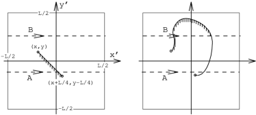
Figure 7: (Left): A $x^{\prime}-y^{\prime}$ plane, where branch cut of ${\rm Im}\log\zeta(\vec{r}^{\prime}-\vec{r})$ runs from $(x,y)$ to $(x+\frac{L}{4},y-\frac{L}{4})$. The shaded side of it is for $-\frac{\pi}{4}-$ while the other side is for $-\frac{9\pi}{4}+$. (Right): One can easily convince oneself that eq. (73) is independent from a specific choice of the branch cut.

To summarize this section, we argue that the successive application of the disorder operator (DOP) along those arbitrary paths which parallel to its branch cut is equivalent to twisting the boundary condition of the system.

VI Summary and Discussions

Based on the duality picture between 2D superconductivity and insulator, we proposed in this paper the disorder operator as a possible candidate for an order parameter of the 2D insulating state, which is valid for arbitrary 2D lattice models. Namely, the change of phase of our disorder operator along a closed loop is nothing but the doped particle density inside this loop. Thus, one can naturally introduce the disorder operator (DOP) as the dual counterpart of the superconducting order parameter.

To inspect the validity of this conjecture, we evaluated the expectation value of this non-local operator in band metal (Sec. III) and in band insulators/gapped mean-field ordered state (Sec. IV). Thereby, we observed that the expectation value of the DOP actually vanishes for a wide class of band metals in the thermodynamic limit. As for band insulators, we estimated its expectation value perturbatively w.r.t. a weak $\vec{k}$-dependence of periodic parts of Bloch w.f., bearing in mind the atomic limit or weak delocalized insulating state close to this limit. Thereby, we found that the DOP is characterized by the localization length $\bar{\xi}$ as $e^{-\frac{\pi^{2}}{2}\bar{\xi}^{2}}$. This localization length is always finite in insulators, while diverges in the presence of F.S. Thus, these two theoretical observations, i.e. in the metallic case and in the weakly delocalized insulating case, naturally lead us to speculate that the expectation value of the DOP in insulators could be always characterized by the same form, although our derivation in the insulator side is valid only for small $\bar{\xi}$. This speculation must be checked in future, with a help of numerics or another analytic scheme of evaluating determinants.

One might also wonder about the behaviour of the DOP in other electronic states, such as superconductors (SC). As for these off-diagonal long range order states (ODLRO), we expect that its expectation value should also vanish lee1 ; lee2 ; fisher ; balents1 ; balents2 ; tesanovic , from the simple quantum mechanical commutation relation between a local density and creation operator, i.e. $[\rho_{\vec{r}_{1}},c^{\dagger}_{\vec{r}_{2}}]=\delta_{\vec{r}_{1},\vec{r}_{2}}c^{\dagger}_{\vec{r}_{2}}$. Namely, the particle number at each site $\rho_{\vec{r}}$ and the phase part of the SC order parameter, e.g. $c^{\dagger}_{\vec{r},\uparrow}c^{\dagger}_{\vec{r},\downarrow}$, are canonical conjugate to each other. Thus, in such an ODLRO where $c^{\dagger}_{\vec{r},\uparrow}c^{\dagger}_{\vec{r},\downarrow}$ is condensed uniformly, the particle number for each site is totally undermined in an entire system. Since the local electronic polarization $\vec{a}(\vec{r})$ and phase part of the DOP, i.e. $\ln\eta(\vec{r})$, are given in terms of the linear combination of these local electron densities, they should be also indefinite. In other word, the DOP should not acquire a finite amplitude in these ODLRO states.

The standard approach of detecting insulating states (and also superconducting states) is to measuring the ground state energy variation w.r.t. the infinitesimally small Aharonov-Bohm (AB) phase inserted in parallel with systems kohn ; resta1 ; resta2 ; scalapino . In order to make a connection to these conventional approaches, we prove that applying the DOP successively along a closed path also eventually ends up with the AB phase inserted in parallel to the 2D plane.

ground state w.f.	band metal			band insulator/gapped m-f state
type of F.S./ localization length	type. O	type. A or type. B	type. AB	general $\bar{\xi}$	small $\bar{\xi}$
single band	$e^{-0.11\cdot N_{e}}$	$<e^{\alpha}\cdot e^{-0.11\cdot N_{e}}$	$-$
m-b. w/o. filled bands	$e^{-0.11\cdot N_{e}}$	$<e^{\alpha}\cdot e^{-0.11\cdot N_{e}}$	$-$	$-$	$e^{-\frac{\pi^{2}}{2}\bar{\xi}^{2}}$
m-b. w. filled bands	$-$	$-$	$-$

Table 2: Summary of Sec. III and IV. “m-b.” denotes “multiple band”. Type. O, type. A(B) and type. AB denotes a type of the F.S. of 2D metal (See Fig. 4). $\bar{\xi}\equiv\frac{\xi}{\rm a}$ denotes a localization length along the $\mu$-direction (see eqs. (53,54) for its definition). “$-$” is the case which we cannot access by our analytical scheme.

Observing these several circumstantial evidences including the connection with the conventional approach, we believe, in spite of its complexness stemming from its non-locality, that the DOP is finite only in an insulator. Then, turning back to our original motivations, i.e. microscopic identification of the counterpart of magnetic penetration depth and coherence length, we are now allowed to push forward a naive thought on this primary motivations. We expect that the localization length $\bar{\xi}$ characterizes not only the expectation value of the DOP in insulating states, but it also specifies the counterpart of the magnetic penetration depth, by the following reasons. Notice, from eq. (54), that the localization length measures how easily the localized electrons constituting the background non-doped insulating w.f. could be polarized, when an external electric field is applied, or in other words when a test charge is introduced into this system. When this test charge is regarded as a single (few) doped particle, the polarizability of the background insulating electrons then could be transcribed into how easily a single doped particle push away these background electrons and acquires its own seat within a bulk, or in other words, forming a vortex within a bulk. Thus, we expect that there should be a certain amount of positive correlation between the localization length $\bar{\xi}$ measured w.r.t. non-doped gapped mean-field ordered w.f. and the counterpart of the magnetic penetration depth in its weakly doped regions. These speculation could be directly judged, when one construct a Ginzburg-Landau type theory for doped 2D insulating state, by using this non-local field, or alternatively, when calculating its multi-point correlation functions, w.r.t. the non-doped insulating w.f..

Appendix A Contribution from the uniform background

When we prove our DOP indeed vanishes in a band metal, it is crucial that the contribution from the uniform background $\langle 0|\eta(\vec{r})|0\rangle$ overkills the contribution from $\det\zeta^{\prime}$, i.e. $|\langle 0|\eta(\vec{r})|0\rangle|\ll e^{-\frac{\ln 2}{2}N_{e}}$. Therefore, in this appendix, we will estimate the contribution from the uniform background,

$$-{\rm ln}\langle 0|\eta(\vec{r})|0\rangle=\frac{N_{e}}{N_{b}N^{2}}\sum_{\vec{r}^{\prime}}\times$$

$$\ \ {\rm ln}\big{[}-i(e^{i\frac{2\pi}{N\rm a}(x^{\prime}-x-x_{0})}-1)+(e^{i\frac{2\pi}{N\rm a}(y^{\prime}-y-y_{0})}-1)\big{]},$$

(76)

up to the order of ${\cal O}(1)$ and prove that this is indeed the case. This summation can be replaced by the integral, as far as $O(L^{2})$ is concerned:

$$-\ln\langle 0|\eta(\vec{r})|0\rangle=\frac{N_{e}}{N_{b}N^{2}}\cdot N_{b}\sum_{x^{\prime},y^{\prime}={\rm a}}^{N\rm a}\times$$ (77)

$$\ \ {\rm ln}\big{[}-i(e^{i\frac{2\pi}{N\rm a}(x^{\prime}-x_{0})}-1)+(e^{i\frac{2\pi}{N\rm a}(y^{\prime}-y_{0})}-1)\big{]}$$

$$= \frac{N_{e}}{4\pi^{2}}\int_{0}^{2\pi}d\theta_{x}\int_{0}^{2\pi}d\theta_{y}\ {\rm ln}\big{[}i+e^{i\theta_{x}}-1+e^{i\theta_{y}}\big{]}$$

$$= N_{e}\ \oint_{|z|=1}\frac{dz}{2\pi i}\oint_{|z^{\prime}|=1}\ \frac{dz^{\prime}}{2\pi i}\ \frac{{\rm ln}\big{[}z^{\prime}-z_{1}(z)\big{]}}{z\cdot z^{\prime}},$$

where we introduced complex variables $z\equiv e^{i\theta_{x}}$, $z^{\prime}\equiv e^{i\theta_{y}}$ and $z_{1}(z)\equiv-z+1-i$. The additional factor $N_{b}$ in the 1st line comes from the summation within the unit cell. Then, we will first divide the above $z$-integral into the following two parts, according as the position of $z_{1}(z)$ in the complex plane;

$$\oint_{|z|=1}\frac{dz}{2\pi i}=\int_{C_{>}}\frac{dz}{2\pi i}+\int_{C_{<}}\frac{dz}{2\pi i}.$$ (78)

Namely, the region $C_{>,<}$ are defined as follows (see Fig. 8):

$$C_{<} \equiv \{z\ |\ |z|=1,\ |z_{1}(z)|<1\},$$

$$C_{>} \equiv \{z\ |\ |z|=1,\ |z_{1}(z)|>1\}.$$

Figure 8: Two integral paths w.r.t. $z$, $C_{<}$ and $C_{>}$

We can easily see that the 2nd term in eq. (78) does not contribute to the real part of eq. (77), by choosing the branch cut of the logarithm, i.e. $\log[z^{\prime}-z_{1}]$, so that it depends on $z_{1}$. Namely, let it run from $z_{1}$ to infinity passing through $\frac{z_{1}}{|z_{1}|}$ (see in Fig. 9). Note that the real part of eq. (77) is free from the specific choice of the branch cut. According as this choice, we will decompose the $z^{\prime}$-integral into the following four parts:

$$\oint_{|z^{\prime}|=1}\ \frac{dz^{\prime}}{2\pi i}=\biggr{(}\oint_{C}-\int_{C_{1}}-\oint_{C_{2}}-\int_{C_{3}}\biggl{)}\cdot\frac{dz^{\prime}}{2\pi i},$$ (79)

where the closed path $C$ is the bold loop depicted in Fig. 9 and

$$C_{1} \equiv \big{\{}z^{\prime}\ |\ {\rm arg}\ln z^{\prime}={\rm arg}\ln z_{1}+0,\ |z_{1}|<|z^{\prime}|<1\big{\}},$$

$$C_{2} \equiv \big{\{}z^{\prime}\ |\ |z^{\prime}-z_{1}|=+\epsilon\big{\}},$$

$$C_{3} \equiv \big{\{}z^{\prime}\ |\ {\rm arg}\ln z^{\prime}={\rm arg}\ln z_{1}-0,\ |z_{1}|<|z^{\prime}|<1\big{\}}.$$

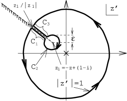
Figure 9: Dotted line emitting from $z_{1}$ to infinity is the branch cut of $\ln[z^{\prime}-z_{1}]$ which we have chosen in eq. (79). $\arg\ln[z^{\prime}-z_{1}]$ takes $+0i$ in the shaded side of this dotted line while $2\pi$ in the other side.

First of all, the third term in the l.h.s. of eq. (79) clearly vanishes, when $\epsilon$ is taken to be infinitesimally small:

$$\oint_{C_{2}}\frac{dz^{\prime}}{2\pi i}\ \frac{{\rm ln}\bigl{[}z^{\prime}-z_{1}\bigr{]}}{z^{\prime}}\cong\frac{i}{2\pi}\frac{\epsilon}{z_{1}}\int_{0}^{2\pi}d\phi\ e^{i\phi}\phi,$$ (80)

where $z^{\prime}-z_{1}\equiv\epsilon e^{i\phi}$. As the integrand in eq. (77), seen as a function of $z^{\prime}$, has no more pole than $z^{\prime}=0$ inside $C$, the first term in eq. (79) reads:

$$\oint_{C}\frac{dz^{\prime}}{2\pi i}\ \frac{{\rm ln}\bigr{[}z^{\prime}-z_{1}\bigl{]}}{z^{\prime}}={\rm ln}|z_{1}|+i\pi.$$ (81)

Due to our choice of the branch cut, the second and fourth terms in eq. (79) can be substantially simplified:

$$\int_{C_{1}}\frac{dz^{\prime}}{2\pi i}\frac{{\rm ln}|z^{\prime}-z_{1}|+0\cdot i}{z^{\prime}}\ +\ \int_{C_{3}}\frac{dz^{\prime}}{2\pi i}\frac{{\rm ln}|z^{\prime}-z_{1}|+2\pi i}{z^{\prime}}$$

$$\hskip 68.28644pt=\ \int_{C_{3}}dz^{\prime}\frac{1}{z^{\prime}}={\rm ln}|z_{1}|$$ (82)

Then, by combining eq. (81) and eq. (82), we finally obtain the 2nd term of eq. (78) as,

$$\int_{C_{<}}\frac{dz}{2\pi i}\frac{1}{z}\oint_{|z^{\prime}|=1}\frac{dz^{\prime}}{2\pi i}\frac{{\rm ln}\big{[}z^{\prime}-z_{1}\big{]}}{z^{\prime}}$$

$$=\frac{1}{2}\int_{C_{<}}\frac{dz}{z}=\frac{i}{2}\int_{-\frac{\pi}{2}}^{0}dk=\frac{\pi}{4}i.$$ (83)

Thus, as far as the real part is concerned, there is no contribution to eq. (77), when $z$ is located on $C_{<}$. Then we will concentrate on the case where $z$ is located on $C_{>}$.

When $z$ on $C_{>}$, $z^{\prime}$-integral can be easily done;

$$\int_{C_{>}}\frac{dz}{2\pi i}\frac{1}{z}\oint_{|z^{\prime}|=1}\frac{dz^{\prime}}{2\pi i}\frac{{\rm ln}\big{[}z^{\prime}-z_{1}(z)\big{]}}{z^{\prime}}$$

$$\ \ =-\int_{C_{>}}\frac{dz}{2\pi i}\frac{{\rm ln}\big{[}-1+i+z\big{]}}{z}$$

$$\ \ =\frac{3}{8}{\rm ln}2+\frac{1}{\pi}\sum_{n=1}^{\infty}\frac{1}{n^{2}}\big{(}\frac{1}{\sqrt{2}}\big{)}^{n}\sin\big{(}\frac{n\pi}{4}\big{)}+i\frac{9\pi}{16}$$

$$\ \ =0.464847699170805...+i\frac{9\pi}{16}.$$ (84)

Then, as far as the order of ${\cal O}(L^{2})$ is concerned, logarithm of $|\langle 0|\eta(\vec{r})|0\rangle|$ can be estimated to be

$$\ln|\langle 0|\eta(\vec{r})|0\rangle|=-0.464847...\times N_{e}+{\cal O}(L).$$ (85)

Next, we will estimate the ${\cal O}(L)$ contribution to ${\rm ln}\langle 0|\eta(\vec{r})|0\rangle$, which turns out to be also pure imaginary. ${\cal O}(L)$ contribution comes from the error due to the replacement of the summation given in eq. (76) by the integral given in eq. (77). This error can be then estimated by the summation of the first derivative of integrand in eq. (77) w.r.t. $\theta_{x}$ and/or $\theta_{y}$. In other words, its leading order correction is always proportional to the following integrals with some real-valued coefficients,

$$\int_{0}^{2\pi}\int_{0}^{2\pi}\frac{d\theta_{x}d\theta_{y}}{4\pi^{2}}\frac{\partial}{\partial\theta_{\mu}}\Big{\{}{\rm ln}\big{[}i+\ e^{i\theta_{x}}-1+e^{i\theta_{y}}\big{]}\Big{\}},$$ (86)

where $\mu=x,y$.

Taking the branch cut of ${\rm ln}\big{[}i+\ e^{i\theta_{x}}-1+e^{i\theta_{y}}\big{]}$ as in Fig. 10, one can easily understand these correction are pure imaginary. Let us see this, taking $\mu=x$ for example.

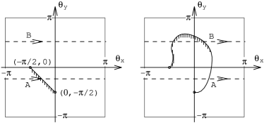
Figure 10: (Left): A $\theta_{x}$-$\theta_{y}$ plane, where branch cut of ${\rm ln}\big{[}i+\ e^{i\theta_{x}}-1+e^{i\theta_{y}}\big{]}$ runs from $(-\frac{\pi}{2},0)$ to $(0,-\frac{\pi}{2})$. The shaded side of it is for $-\frac{\pi}{4}-$ while the other side is for $-\frac{9\pi}{4}+$. (Right): One can easily convince oneself that eqs. (58,87) are independent from a specific choice of the branch cut.

In the case of $\theta_{y}\notin[-\frac{\pi}{2},0]$ (see the line B in Fig. 10), the $\theta_{x}$-integral always vanishes due to the periodicity of ${\rm ln}\big{[}i+\ e^{i\theta_{x}}-1+e^{i\theta_{y}}\big{]}$. On the other hand, in the case of $\theta_{y}\in[-\frac{\pi}{2},0]$, the integral w.r.t. $\theta_{x}$ meets $2\pi$ jump when its integral path crosses the branch cut which extends from $(-\frac{\pi}{2},0)$ to $(0,-\frac{\pi}{2})$ (see the line A in Fig. 10). Then, when integrating w.r.t. $\theta_{x}$ over $[-\pi,\pi]$, we obtain $2\pi i$ as the surface term in the latter case. As a result, the above integrals with $\mu=x$ reads:

$$\frac{1}{4\pi^{2}}\int_{-\frac{\pi}{2}}^{0}d\theta_{y}\times 2\pi i=\frac{i}{4}.$$ (87)

In a same way, we can easily see that the integral with $\mu=y$ also turns out to be $\frac{i}{4}$. After all, the error which stems from replacing the summation of eq. (76) by the integral given in eq. (77) can have a contribution of the order ${\cal O}(L)$, but it is always pure imaginary. Thus, when it comes to ${\rm ln}|\langle 0|\eta(\vec{r})|0\rangle|$, there is no ${\cal O}(L)$ contributions.

To summarize this appendix, ${\rm ln}|\langle 0|\eta(\vec{r})|0\rangle|$ is estimated up to the order of ${\cal O}(1)$ and it reads:

$$\ln|\langle 0|\eta(\vec{r})|0\rangle|=-0.464847...\times N_{e}+{\cal O}(1),$$ (88)

which is actually less than $-\frac{\log 2}{2}N_{e}$.

References

- (1) K.M. Lang, V. Madhavan, J.E. Hoffman, E.W. Hudson, H. Eisaki, S. Uchida and J.C. Davis, Nature 415, 412, (2002)
- (2) T.Hanaguri, C. Lupien, Y. Kohsaka, D.H. Lee, M. Azuma, M. Takano, H. Takagi, J.C. Davis, Nature 430, 1001, (2004)
- (3) M. Uehara, S. Mori, C.H. Chen, S-W. Cheong, Nature 399, 560, (1999)
- (4) D.H. Lee, cond-mat/0208490
- (5) D.H. Lee and S.A. Kivelson, Physical Reveiw B 67, 024506, (2003)
- (6) M.P.A. Fisher and D.H. Lee, Physical Review B 39, 2756, (1989)
- (7) L. Balents, M.P.A. Fisher and C. Nayak, International Journal of Modern Physics B 12, 1033, (1998)
- (8) L. Balents, M.P.A. Fisher and C. Nayak, Physical Review B 60, 1654, (1999)
- (9) Z. Tesanovic, Physical Review Letters 93, 217004, (2004)
- (10) W. Kohn, Physical Review A 133, A171, (1964)
- (11) E. K. Kudinov, Soviet Physics - Solid State, 33, 1299, (1991)
- (12) I. Souza, T. Wilkens and R.M. Martin, Physical Review B 62, 1666, (2000)
-
(13)
Accurately speaking,
is not exactly same
as . However, as
shown in appendix. A, their difference is at most
order , when it comes to their real part.
Thus, the amplitude of our DOP in the atomic limit
is also of , i.e.
Furthermore, this -error depends only on the specific choice of the position of , introduced in eq.(7), within each unit cell and does not contains any information of the ground state w.f.. Thus we do not care about this contribution henceforth.(89) - (14) P. G. de Genne, Superconductivity of metals and alloys (Perseus Books, Massachusetts, 1999).
- (15) E. Fradkin and L. P. Kadanoff, Nuclear Physics B 170, 1 (1980).
- (16) S. Kivelson, Physical Review B 26, 4269, (1982)
- (17) N. Marzari and D. Vanderbilt, Physical Review B 56, 12847, (1997)
- (18) R. Resta Physical Review letters 80, 1800 (1998).
- (19) R. Resta and S. Sorella, Physical Review Letters 82, 370, (1999).
- (20) D.J. Scalapino, S.R. White, S.C. Zhang, Physical Review B 47, 7995 (1993); Physical Review Letters 68, 2830 (1992).
- (21) J. Anandan and Y. Aharonov, Physical Review Letters 65, 1697 (1990).