Solution of the Unanimity Rule on exponential, uniform and scalefree networks:
A simple model for biodiversity collapse in foodwebs

Abstract

We solve the Unanimity Rule on networks with exponential, uniform and scalefree degree distributions. In particular we arrive at equations relating the asymptotic number of nodes in one of two states to the initial fraction of nodes in this state. The solutions for exponential and uniform networks are exact, the approximation for the scalefree case is in perfect agreement with simulation results. We use these solutions to provide a theoretical understanding for experimental data on biodiversity loss in foodwebs, which is available for the three network types discussed. The model allows in principle to estimate the critical value of species that have to be removed from the system to induce its complete collapse.

I Introduction

Unanimity rule (UR) is generally associated with models, where a (binary) state of an atom or agent can change only if all of its direct neighbors are in the other state, respectively. Usually UR is formulated in a network framework, where a node becomes ’activated’ only if all the nodes pointing to it – through directed links – are ’activated’. These models have attracted some recent interest because of a number of important real world applications. Maybe the most relevant example is the modeling of biodiversity based on foodwebs. Species are nodes in this web. If one species is food for another species this is indicated by a directed link in the foodweb, pointing from the eaten species to the eater. Usually one species does not depend on a single other species but in general has a more diversified menue. In the picture of the foodweb this means that each node is pointed at from several other neighbors. Imagine that all species in a hypothetical foodweb exist in one of two states: alive or extinct. If all the neighbors pointing to a particular node $i$, are extinct the node itself has no more food to live on and will go extinct in the next timestep as well; the relation to the UR becomes apparent. UR has been studied experimentally in actual foodwebs to model biodiversity loss dunne1 ; dunne2 . Earlier efforts on modeling foodweb topology and its fragility have been conducted with respect to clustering, fragmentation, robustness, and degree distribution under the assumptions of random and non-random extinction of species SoleMontoya_2001 . In MontoyaSole_2002 small world effects are investigated and it was concluded that foodwebs are not random networks with Poissonian degree distribution. Niche models – as a method of sampling surrogate foodwebs – are studied in Martinez2000 ; CamachoGuimera_2002_PRL ; StoufferCamacho_2006 which (in the low connectancy limit) display robust scaling properties of foodwebs which is in good agreement with data from several field studies, see e.g. field . Further, their conclusion that the degree distribution of foodwebs decays exponentially rather than scale-free is in good agreement with dunne1 ; dunne2 . Studies concerned with the robustness of foodwebs generally use the UR as an update mechanism, propagating initial extinction of species.

Surprisingly, the dynamics of Unanimity Rule, which is a generalization of the Majority Rule of opinion dynamics redner ; red ; lambi ; lambi1 ; lambi2 and reminds on features of the Voter model voter0 ; voter1 ; voter2 ; voter3 , the Axelrod model axelrod ; axelrod2 as well as of Boolean networks kauffman ; kauz , is poorly known hanel ; hanel2 and has been put on a more mathematical basis only recently lambiotte07 . The unanimity model as presented there can also be viewed as a limiting case of a model for decision making scenarios watts0 . Note that UR differs from these previous models by the fact that it is irreversible, i.e. once a node has reached the activated state, it remains in it. This irreversibility of UR makes it an excellent candidate not only for modeling biodiversity as above but also for the adoption of new technologies, such as MMS mms , by interacting customers. Technological standards are generally irreversible once they are adopted by a population. Another specificity of UR is the fact that it is purely deterministic, i.e. once the topology of the underlying network is fixed and an initial number of nodes are activated, the entire dynamics is determined. In contrast, the Voter model, when applied to complex networks, involves a random step when a node chooses an interaction partner among its neighbors. Similarly, in the Majority Rule, a node choses randomly between two nodes among its neighbors to form a majority triplet.

In this paper we start from the dynamical equation for UR on networks and solve it analytically for the special cases of exponenential and scale free networks. We then compare the results with experimental findings obtained from actual foodwebs dunne1 ; dunne2 .

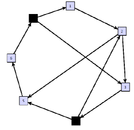
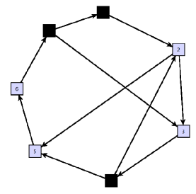
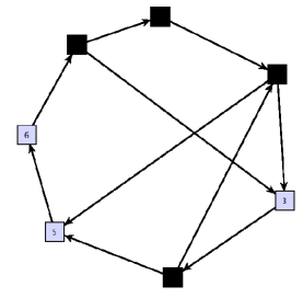
Figure 1: First two steps of UR starting from an initial network of 7 nodes, 2 of them being activated. Initially there is only one node among the non-activated nodes that satisfies the unanimity rule. It gets therefore activated at the first time step. At that time, there is a new node whose 2 incoming links come from activated nodes. It gets activated at the second time step. This system gets fully activated at the fourth time step. In the context of foodwebs for example node 2 eats species 1 and 4, and serves as food for species 3 and 5. A black node means that it is extinct. (From lambiotte07 ).

II Unanimity Rule

UR is implemented amongst agents in a network composed of $N$ nodes connected through $L$ directed links. Each node exists in one of two states: activated or inactivated. The number of nodes with indegree $i$ (number of links pointing to it) is denoted by $N_{i}$ and depends on the underlying network structure, i.e. the indegree distribution is given by $p_{i}=N_{i}/N$. It is a fixed quantity that does not evolve with time. The fraction of activated nodes at time $t$ we denote by $a_{t}$, for the fraction of activated nodes with an indegree $i$, we write $a_{i,t}$. Initially (at $t=0$) there is a fraction of $a_{0}$ activated nodes. Obviously

$$a_{t}=\sum_{i}p_{i}a_{i,t}$$ (1)

holds. The unanimity rule is defined as shown in Fig. 1. If all the links arriving to an inactivated node $i$ originate from nodes which are activated at $t-1$, $i$ gets activated at $t$. Otherwise, it remains inactivated. At each time step every node is considered for an update, the dynamics is synchronous. The process is iterated until the system reaches a stationary, frozen state, characterized by an asymptotic value $a_{\rm final}\equiv a_{\infty}$. The UR problem is to predict $a_{\infty}$ from the knowledge of the $a_{0}$ and the structure (indegree distribution) of the network.

To solve problems of this nature a two step approach was suggested hanel ; hanel2 : first map the problem onto an update equation, second find the asymptotic solutions of the latter. To derive the update equation, note that the probability that $i$ randomly chosen nodes are initially activated, is $a^{i}_{0}$ ($i$ is an exponent). The average number of nodes with indegree $i$ and which respect the unanimity rule is therefore $N_{i}a^{i}_{0}$. Among these nodes, $N_{i}a_{0}a^{i}_{0}$ were already activated initially. This is due to the fact that the total number of nodes with (in)degree $i$ which are initially activated is $N_{i}a_{0}$. Consequently, the number of nodes that gets activated at the first time step is

$$\Delta_{i,0}=\left(N_{i}-N_{i}a_{0}\right)a^{i}_{0}\quad,$$ (2)

and, on average, the total number of occupied nodes with indegree $i$ evolves as

$$A_{i,1}=A_{i,0}+\Delta_{i,0}\quad.$$ (3)

At the next time step, the average number of nodes with indegree $i$, which respect the unanimity rule and which are outside the initial set is $(N_{i}-N_{i}a_{0})a^{i}_{1}$. Among those nodes, $\Delta_{i,0}$ have already been activated during the first time step, so that the average number of nodes which get activated at the second time step is

$$\Delta_{i,1}=(N_{i}-N_{i}a_{0})(a^{i}_{1}-a^{i}_{0})\quad.$$ (4)

Note that Eq. (4) is valid because no node in $\Delta_{i,1}$ also belongs to $\Delta_{i,0}$. This is due to the fact that each node can only be activated by one combination of $i$ nodes in our model, so that no overlap is possible between $\Delta_{i,1}$ and $\Delta_{i,0}$. By iterating it is straightforward to show that the contributions $\Delta_{i,t}$ read

$$\Delta_{i,t}=(N_{i}-N_{i}a_{0})(a^{i}_{t}-a^{i}_{t-1})\quad,$$ (5)

with $a_{-1}=0$, by convention. The number of activated nodes evolve as $A_{i,t+1}=A_{i,t}+\Delta_{i,t}$, and by dividing by $N_{i}$, one gets the equations for the fraction of activated nodes $a_{i}\in[0,1]$

$$a_{i,t+1}=a_{i,t}+(1-a_{0})(a^{i}_{t}-a^{i}_{t-1})=a_{i,0}+(1-a_{0})a_{t}^{i}\quad.$$ (6)

Now $a_{t}$ is the convex sum of Eq. (6) with weights according to the indegree distribution $p_{i}$, i.e. $a_{t}=\sum_{i}p_{i}a_{i,t}$. Finally we get for the update equation

$$a_{t+1}=a_{0}+(1-a_{0})\sum_{i}p_{i}a^{i}_{t}\quad.$$ (7)

Numerical solutions for $t\to\infty$ are found in Fig. 2 for several different indegree distributions $p_{i}$ (symbols).

III Exponential and Scalefree

Let us focus on the special choices of the exponential ($p_{i}\propto e^{-\lambda i}$), and scalefree ($p_{i}\propto i^{-\lambda}$), indegree distributions, to analytically uncover the behavior of Eq. (7). The simpler cases, $p_{i}=\delta_{i1}$ and $p_{i}=\delta_{i2}$ have been solved in lambiotte07 .

For the exponential case we have to find an expression for the term $\sum_{i=1}^{M}p_{i}a^{i}_{t}$, where $M$ is the maximum indegree, i.e. $M\leq N$. With the exact identity, $\sum_{i=1}^{M}c^{i}=c(1-c^{M})/(1-c)$, the exact asymptotic equation for the exponential case is found to be

$$a_{\infty}=a_{0}+(1-a_{0})a_{\infty}\left(\frac{1-e^{-\lambda}}{1-e^{-\lambda M}}\frac{1-\left(e^{-\lambda}a_{\infty}\right)^{M}}{1-e^{-\lambda}a_{\infty}}\right)\quad,$$ (8)

where we first have set $c=\exp(-\lambda)a_{\infty}$ for the non-normalized contribution of $p_{i}a_{t}^{i}$, and second $c=\exp(-\lambda)$, to account for the norm of the distribution $p_{i}$. Finally we have taken the limit $t\to\infty$.

We get two important limiting cases: First, the uniform distribution is recovered as the limit $\lambda\to 0$,

$$a_{\infty}=a_{0}+(1-a_{0})\frac{a_{\infty}}{M}\left(\frac{1-a_{\infty}^{M}}{1-a_{\infty}}\right)\quad,$$ (9)

where we have used the fact that $\lim_{\lambda\to 0}(1-\exp(-M\lambda))/(1-\exp(\lambda))=M$.

Second, the large system limit $M\to\infty$ is

$$a_{\infty}=a_{0}+(1-a_{0})a_{\infty}\left(\frac{1-e^{-\lambda}}{1-e^{-\lambda}a_{\infty}}\right)\quad.$$ (10)

The scalefree case is treated similarly. We approximate $\sum_{i=1}^{M}i^{-\lambda}a_{t}^{i}\approx 1+\int_{3/2}^{M+1/2}dx\,\,x^{-\lambda}a_{t}^{x}$ and $\sum_{i=1}^{M}i^{-\lambda}\approx 1+\int_{3/2}^{M+1/2}dx\,\,x^{-\lambda}$. Defining the two-sided incomplete gamma-function as $\gamma(a,b,x)=\int_{a}^{b}dy\,\,y^{x-1}\exp(-y)$ the asymptotic solution for the scalefree unanimity rule reads

$$a_{\infty}=a_{0}-(1-a_{0})\bar{\lambda}\frac{1+\left|a_{\infty}\right|^{\bar{\lambda}}\gamma(\frac{3}{2}\left|a_{\infty}\right|,(M+\frac{1}{2})\left|a_{\infty}\right|,-\bar{\lambda})}{\left(M+\frac{1}{2}\right)^{-\bar{\lambda}}-\left(\frac{3}{2}\right)^{-\bar{\lambda}}-\bar{\lambda}}\quad,$$ (11)

where $\bar{\lambda}=\lambda-1$. The quality of the results for the exponential, uniform and scalefree cases is seen in Fig. 2, where the asymptotic value is plotted against the initial $a_{0}$. Points represent the numerical solution to Eq. (7) for realizations of networks of the characteristics specified in the figure caption. Solid lines are the analytical results from Eqs. (8), (9) and (11). These equations show that the larger the exponents $\lambda$ (for exponential and scalefree) the larger the critical value (where the plateau at $1$ is first reached) becomes. Similarly, the larger $M$ the larger the critical value.

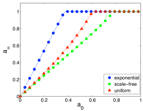
Figure 2: Asymptotic solutions, $a_{\infty}$, of the UR on three types of networks vs. initial condition $a_{0}$. Symbols represent the numerical solutions of Eq. (7). The networks used for this solutions have been generated with $\lambda=-1$, $M=10$ for the exponential, $M=4$ for the uniform and $\lambda=-0.5$, $M=10$ for the scalefree case. Lines are the theoretical results of Eqs. (8), (9) and (11), for the same parameters. The critical value is where the plateau at $1$ is reached (all species extinct).

IV Experiment

In dunne1 ; dunne2 experimental results on foodwebs are presented, which are the outcomes from numerous field studies, see References 9,11,15,28-37 in dunne2 . In dunne1 the number of species having died out as a result of the initial removal of a given fraction of the total population is presented. This constitutes a UR on networks, where – in our notation – the fraction of activated links $a_{t}$ are the ones that have died out after $t$ timesteps. The reported networks there have been exponential, uniform and scalefree. We have re-drawn the data from dunne1 for two examples for each network type in Fig. 3 (symbols). Unfortunately, the network parameters can not get reconstructed from dunne2 . The data presented contains in- and outdegrees mixed together, which makes it impossible to estimate $\lambda$ and $M$ for the indegree only (which is needed for the UR). The lines represent our theoretical results where we have estimated the parameters in the following way. For the exponential we fixed $\lambda$ to the values reconstructed from Fig. 2 in dunne2 , and varied $M$ until good fit was obtained. Of course $M_{\rm opt}$ is less than $M$ reported in Fig. 2 of dunne2 . The uniform case turned out to be optimal with $M_{\rm opt}$ about half of the reported value, the scalefree case was fitted after fixing $M$ to about half of the reported case and varying $\lambda$.

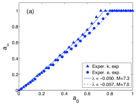
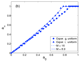
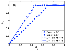
Figure 3: Experimental data from dunne1 ; dunne2 (and references therein), for the number of asymptotically died out species on measured exponential (a), uniform (b) and scalefree (c) distributions (for randomly removed species). Lines are curves from our theoretical solutions with parameters as explained in the text.

V Discussion

We have solved the UR on exponential, uniform and scalefree networks. These solutions relate the structure of the underlying network together with an initial loss of diversity, $a_{0}$ with the final diversity in the system. Once the structure of the underlying network is known, these solutions allow further to find the critical value of initial ’species removal’ $a_{0}^{\rm crit}$ at which (and beyond which) a total collapse of the system will appear. The dynamics on foodwebs (who eats whom) is a particular example of this UR, the reported underlying networks are of exponential, uniform and scalefree nature. We have shown that not only do our results compare well with simulations but also with actual experimental data. The message of this work is to point out the potential danger of uncontrolled anthropogenic species removal.

Acknowledgements We are grateful to support from the Austrian Science Foundation projects P17621 and P19132.

References

- (1) J.A. Dunne, R.J. Williams and N.D. Martinez, Ecology Letters 5, 558-567 (2002).
- (2) J.A. Dunne, R.J. Williams and N.D. Martinez, Proc. Natl. Acad. Sci. USA 99, 12917-12922 (2002).
- (3) R.V. Sole and J.M. Montoya, Proc. Roy. Soc. Lond. B 268 , 2039-2045 (2001).
- (4) J.M. Montoya and R.V. Sole, J. theor. Biol. 214, 405-412 (2002).
- (5) R.J. Williams and N.D. Martinez, Nature 404, 180 (2000).
- (6) J. Camacho, R. Guimera and L.A.N. Amaral, Phys. Rev. Lett. 88, 228102 (2002); Phys. Rev. E 65, 030901 (2002).
- (7) D.B. Stouffer, J. Camacho and L.A.N. Amaral, PNAS 103 50, 19015-19020 (2006).
- (8) S.J. Hall and D. Rafaelli, J. Anim. Ecol. 60, 823-842 (1991); M. Huxham, S. Beaney and D. Rafaelli, Oikos 76, 284-300 (1996).
- (9) P. L. Krapivsky and S. Redner, Phys. Rev. Lett. 90, 238701 (2003).
- (10) M. Mobilia and S. Redner, Phys. Rev. E 68, 046106 (2003).
- (11) R. Lambiotte, M. Ausloos and J. Hołyst, Phys. Rev. E 75, 030101(R) (2007).
- (12) R. Lambiotte, EPL 78, 68002 (2007).
- (13) R. Lambiotte and M. Ausloos, physics/0703266.
- (14) E. Ben-Naim, L. Frachebourg and P. L. Krapivsky, Phys. Rev. E 53, 3078 (1996).
- (15) V. Sood and S. Redner, Phys. Rev. Lett. 94, 178701 (2005).
- (16) C. Castellano, D. Vilone, and A. Vespignani, EPL 63, 153 (2003).
- (17) C. Castellano, V. Loreto, A. Barrat, F. Cecconi and D. Parisi, Phys. Rev. E 71, 066107 (2005).
- (18) R. Axelrod, J. Conflict. Resolut. 41, 203 (1997).
- (19) D. Stauffer, AIP Conference Proceedings 779, 56-68 (2005).
- (20) S. A. Kauffman, The Origins of Order (Oxford University Press, London, 1993).
- (21) M. Huxham, S. Beaney and D. Raffaelli, J. Theor. Bio. 22, 437 467 (1969).
- (22) R. Hanel, S. A. Kauffman and S.Thurner, Phys. Rev. E 72, 036117 (2005).
- (23) R. Hanel, S. A. Kauffman and S.Thurner, arXiv:physics/0703103
- (24) R. Lambiotte, R. Hanel and S. Thurner, arXiv:physics/0612025.
- (25) D. J. Watts, Proc. Natl. Acad. Sci. USA 99, 5766 (2002).
- (26) http://en.wikipedia.org/wiki/Multimedia_Messaging_Service