High-Speed Optical Spectroscopy

Abstract

The large surveys and sensitive instruments of modern astronomy are turning ever more examples of variable objects, many of which are extending the parameter space to testing theories of stellar evolution and accretion. Future projects such as the Laser Interferometer Space Antenna (LISA) and the Large Synoptic Survey Telescope (LSST) will only add more challenging candidates to this list. Understanding such objects often requires fast spectroscopy, but the trend for ever larger detectors makes this difficult. In this contribution I outline the science made possible by high-speed spectroscopy, and consider how a combination of the well-known progress in computer technology combined with recent advances in CCD detectors may finally enable it to become a standard tool of astrophysics.

1 Introduction

High-speed photometry has a long history in optical astronomy. The late 1960s and early 1970s saw the combination of digital recording techniques and photomultiplier tubes to give photon counting high-speed photometry, e.g. Nather:HighSpeed . Equivalent high-speed spectroscopy has never been as straightforward and is still not a standard technique. There are several reasons for this. First, it is technically more difficult and expensive to record spectra at high-speed as one needs fast 2D imagers rather than single pixel devices. An early example, which was developed for faint object spectroscopy but could also take fast spectra, was the Image Photon Counting System (IPCS) Boksenberg:IPCS . The IPCS illustrates a problem typical of high-speed spectroscopy, because although it could take spectra with exposure times well below 1 second, it was rarely used to do so because its design limited its maximum count rate in any given pixel to less than 1 photon/second. A second difficulty of high-speed spectroscopy in the era of the IPCS was simply that it could produce more data than the computer technology of the 1970s and early 1980s could easily deal with; the author of this chapter recalls an observing run on the Anglo-Australian telescope which produced enough magnetic tape to run to and from the local town Coonabarabran 40 km away twice over. Computer technology has since taken enormous strides of course, but the 1980s brought the biggest obstacle of all for high-speed spectroscopy, namely Charge-Coupled Devices (CCDs). Although wonderful detectors in many respects, the CCDs employed in most observatories have two significant disadvantages: they are slow, often taking several tens of seconds to read out, and significant noise is added to each pixel, burying the small signals characteristic of high-speed spectroscopy. The slow readouts of standard CCDs has lead to a small revival of the old photographic method of “trailed spectra” where the target is moved along the slit to give time-resolved spectra Falter:pg1605 ; Schwope:HUAqr1 , but the disadvantages of this method, such as seeing-dependent time-resolution, mean that it is really only a stop gap measure and I will not consider it further.

Despite the problems of CCDs, their other excellent characteristics, in particular their high quantum efficiency (QE), have lead to their complete dominance of optical astronomy, and so the focus of this chapter will be tilted towards the use of CCDs for high-speed spectroscopy. Moreover, CCDs are so dominant that they provide us with an empirical definition of what “high-speed” means when applied to spectroscopy, i.e. any spectroscopic observation that is difficult to carry out with normal CCDs is “high-speed”. This does not always mean very fast: readout noise can make echelle spectroscopy of an 18^th magnitude object difficult to carry out with a time resolution shorter than 10 minutes.

With the above broad definition in mind, an overview is given of the science that high-speed spectroscopy makes possible followed by the technical requirements and the possible application of electron-multiplying CCDs to this area.

2 Scientific Motivation

As the introduction hinted, for a variety of reasons, high-speed spectroscopy has yet to take off fully and many applications exist only in the imagination. There are nonetheless a reasonable number of published examples which give an idea of what to expect, and in addition we have the many applications of high-speed photometry to draw on as a resource when considering what can be learned from high-speed spectroscopy. In this section I will look at what high-speed spectra can tell us when applied to the following phenomena, sticking as far as possible to what is already known:

• pulsating white dwarfs and subdwarf B (sdB) stars

• accreting binary stars

• white dwarf binary stars

Before doing so, it is worth mentioning objects yet to be discovered because surveys are being planned to look for short-timescale variable phenomena which are bound to discover many objects that will need high-speed spectroscopy. Pre-eminent perhaps, although still far-off, is the Large Synoptic Survey Telescope (LSST), in which it is planned to use an $8.4\,$m telescope to survey the observable sky once every 3 nights in 15-second exposures.

2.1 Pulsating white dwarfs and sdB stars

As well demonstrated by helioseismology, pulsations in stars can give us unique insights into stellar structure. The area of asteroseismology tries to use pulsations in other stars in this manner. It is observationally demanding first and foremost because of the need for long, uninterrupted time series in order to obtain clean time series. In the case of white dwarfs and sdB stars, which have pulsation periods of order 100 to 1000 seconds, fairly fast observations are also a requirement. If all goes well, it is possible to pin down stellar parameters with great precision. For instance studies of the pulsating sdB stars PG0014+067, PG1219+534 and Feige 48 have measured their surface gravities to $\sim 1$%, their masses to $\sim 2$% and also determined the masses of their hydrogen envelopes, for which no other method exists, to $\sim 10$% Brassard:PG0014 ; Charpinet:PG1219+534 ; Charpinet:Feige48 . Despite this, even large datasets can leave stars unsolved, especially if they display few pulsation modes, the difficulty being the secure identification of a particular eigenmode with a given frequency.

It is unlikely that spectroscopic data can ever be taken with the same time coverage and uniformity as the photometric data. However spectra can add extra information missing from the photometric studies because the variation of limb darkening with wavelength in combination with the different patterns of different eigenmodes can lead to different variations of pulsation amplitude with wavelength Robinson:G117-B15A . Figure 1 shows

Figure 1: The pulsation amplitudes versus wavelength for spherical harmonics $Y_{lm}$ with different $l$-values. Each curve is normalised by its value at 5500Å. The figure is Fig. 3 taken from Clemens:G29-38

predictions Clemens:G29-38 of the amplitudes of different eigenmodes for the ZZ Ceti star G29-38. This shows that spectra may allow $l=3$ and $l=4$ eigenmodes to be distinguished from $l=1$ and $l=2$ eigenmodes. A signal-to-noise ratio of 1000 only gives a signal-to-noise of 10 in the amplitude spectrum when the amplitude itself is of order one percent as it is in ZZ Ceti stars, and therefore extremely high quality data are needed to separate $l=1$ from $l=2$. Thus this application requires moderately fast data acquisition to resolve the pulsations, but also a large aperture to give high signal-to-noise. Figure 2 shows the result of

Figure 2: Spectra of the first pulsation amplitudes of the ZZ Ceti star G29-38 observed on Keck-II/LRIS by vanKerkwijk:G29-38 . The figure is adapted from Fig. 4 of Clemens:G29-38

4 hours of Keck II/LRIS time devoted to the brightest ZZ Ceti star, G29-38 ($V=13$) vanKerkwijk:G29-38 ; Clemens:G29-38 . The mean spectrum of these data appears almost noiseless Clemens:G29-38 , as might be expected for a bright star on a large telescope, but comparing Figs. 1 and 2 shows how necessary the large aperture is in this case.

This case illustrates another important feature of high-speed spectroscopy: it does not have to be especially “high-speed” by photometric standards to strain the capabilities of standard instrumentation: the data were taken as $700\times 12\,$second exposures, but for each exposure there were a further 12 seconds “deadtime” for readout, etc., so the observations were only 50% efficient. This is quite common; indeed 12 seconds is commendably short in this respect. Reducing deadtime is probably the single most effective way of enabling high-speed spectroscopy and would save countless hours of precious telescope time.

The end result of the work shown in Figs. 1 and 2 is that most of the modes are $l=1$ modes. This shows the power of spectroscopy because in principle this method can be applied to stars showing just a few modes where it would certainly not be possible to unravel the modes purely photometrically.

2.2 Accreting binary stars

I now move on to systems which display variability on much shorter timescales than the white dwarf and sdB pulsators. The shortest dynamical timescales in accreting binaries with compact objects range from $1$ to $10$ seconds in the case of accreting white dwarfs down to about a millisecond in the case of the neutron stars and stellar mass black holes. Variability on seconds timescales is well established from the “dwarf nova oscillations” displayed by dwarf novae during their outbursts. To my knowledge, dwarf nova oscillations have only been observed spectroscopically with sufficient speed to detect them once Steeghs:V2051Oph , but this single observation was enough to show the great diagnostic potential spectra may hold for these poorly-understood but remarkable phenomena.

The variability timescales seen in black-hole and neutron star systems can depend upon the system brightness and instrumental limitations as much as the object. X-ray variability at kilohertz frequencies has been seen in X-ray binaries, while optical variability on timescales well below $0.1$ seconds has been seen in bright systems Motch:GX339-4 . Using ULTRACAM on the Very Large Telescope (VLT) we found significant flaring on timescales of a few seconds in a faint quiescent black-hole accretor (Shahbaz et al, in prep). One can only speculate upon the spectroscopic signatures of this variability at optical wavelengths as no such observations have been made, but it is very likely that there will be some, although in the quiescent black-hole case only an “Extremely Large Telescope” (ELT) would be up to the task. A case of particular interest is the fluorescent Bowen blend emission from the donor stars seen in some X-ray binaries and which in some cases has revealed the donor star for the very first time Steeghs:ScoX-1 . This emission is presumably X-ray driven, and can be expected to respond to X-ray variability; some evidence of this has been obtained using narrow-band photometry with ULTRACAM Casares:echo , but a much cleaner signature could come from high-speed spectra.

A dramatic example of spectral variability from an accreting binary is shown in Fig. 3.

Figure 3: The first and second panels show two of the emission lines of the dwarf nova IP Peg as they are eclipsed, with orbital phase increasing up the plot. The spectra were taken on Subaru during an outburst of IP Peg; the lines are dominated by light from the bright accretion disc during this state. The second panel shows a simple computation of the eclipse of a disc in prograde, Keplerian rotation. Figure adapted from Fig. 2 of Ishioka:IPPeg

This shows the eclipse phases of the white dwarf accretor IP Peg in one of its temporary high states (outburst) Ishioka:IPPeg . The lines from this system come primarily from the accretion disc and have the well-known double-peaked profiles that come from Doppler shifting in accretion discs Horne:Emlines . The spectra plotted cover about 30 minutes and show very large changes as first the approaching side of the disc is obscured, affecting the blue-shifted parts of the lines, followed soon after by their red-shifted counterparts. The right-most panel of Fig. 3 shows a simple model which captures much of the phenomenology of the data while at the same time showing significant discrepancies. The nature of these is not understood although it is possible that the disc during outburst is far from Keplerian in nature. This example is an even starker indication of the problems often faced with facility instruments: IP Peg reaches $V=12$ in outburst, yet despite using the $8\,$m Subaru, the time resolution here was a sluggish 80 seconds, each spectrum consisting of 30 seconds exposure followed by 50 seconds of deadtime. The telescope, instrument and object would have allowed much higher speed than this. Ideally one would want to sample fast enough to resolve structure comparable in size to the white dwarf, which would be about 5 seconds in this case. Unfortunately the detector/data acquisition system was not up to the job, a not-uncommon situation, as instruments are rarely built with high-speed applications in mind.

I finish off this section with a look at Doppler imaging as applied to accreting binary stars in the form of Doppler tomography Marsh:Doppler ; Marsh:doppler_review . Doppler tomography uses the information in line profiles as a function of phase to image binaries. Notable successes have been the discovery of spiral structure in accretion discs during outburst Steeghs:Spiral ; Groot:UGem and the unravelling of the complex accretion structures in the magnetic polar class of accreting white dwarfs Schwope:HUAqr1 . Doppler tomography provides a quantitative illustration of the need for high-speed spectroscopy and is useful in defining requirements for such work. This is because the resolution in Doppler tomography is limited by both spectral and time resolution. If one is aiming for a spatial resolution $\Delta x$, then this imposes the following restrictions on the spectral resolution $R_{\lambda}=\lambda/\Delta\lambda$ and the time resolution $\Delta t$:

$$R_{\lambda} \sim (c/\Omega)(\Delta x)^{-1},$$ (1)

$$\Delta t \sim V^{-1}\Delta x,$$ (2)

where the orbital angular frequency $\Omega=2\pi/P$ where $P$ is the orbital period, and $V$ is the velocity of the feature being imaged. Small $\Delta x$ requires large $R_{\lambda}$ and small $\Delta t$. These relations can be combined into a single one relating spectral and time resolution:

$$\Delta t\sim\Omega^{-1}\frac{c}{V}R_{\lambda}^{-1}.$$ (3)

Taking typical values $P=1.5\,$hours and $V=700\,\mathrm{km}\,\mathrm{s}^{-1}$, and assuming that we are working on a spectrograph with $R_{\lambda}=10$,$000$, then we require $\Delta t<30\,$seconds in order that smearing during the exposures does not degrade the resolution. Equations 1 and 2 imply that the number of counts per detector resolution element per exposure scales as $(\Delta x)^{2}$, and thus Doppler tomography can become challenging even on quite bright objects and large telescopes.

2.3 White dwarf binary stars

For my final example of applications of high-speed spectroscopy I turn to binary stars with white dwarf components. This is another case where there are only a few examples, but where one can point to future applications which will prove tough for even the largest telescopes. Work over the past decade has established the existence of a huge population of detached, close double white dwarfs, with orbital periods of a few days or less Marsh:friends ; Napiwotzki:SPY2 . The shortest period of these is WD0957-666 with $P=88\,$minutes (Fig. 4) Bragaglia:DDs ; Maxted:DDmassratios ; Moran:WD0957-666 .

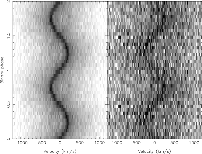
Figure 4: Trailed spectra around H$\alpha$ of the shortest period double white dwarf, WD0957-666, based upon the data of Maxted:DDmassratios . In the left panel, the brightest of the two white dwarfs is clearly seen; the right-hand panel shows the result of subtracting a fit to the brightest star which reveals its companion. The two stars will merge under gravitational radiation in about 200 million years

There are estimated to be of order 100 million such systems in our galaxy, and they should be steadily spiralling towards shorter periods under the action of gravitational wave radiation. The existence of systems such as WD0957-666, which will merge within 200 million years, proves that there must be a population of much shorter period systems that we have yet to detect. This was realised some time ago and it is thought that this population, along with their accreting counterparts, the AM CVn stars, will be the dominant gravitational wave emission sources at frequencies of order $10^{-3}\,\mathrm{Hz}$, right in the waveband of the Laser Interferometer Space Antenna (LISA) Hils:GWR ; Nelemans:GWR0 ; Nelemans:GWR which unlike ground-based detectors is sensitive to gravitational waves of relatively long period . LISA is predicted to be able to detect several thousand of these sources and will be able to narrow down the location of many of them to less than one degree Cooray:DWDs ; Stoeer:DWDs , and it should be possible to optically identify some of them. Optical follow-up can help in the determination of parameters from the LISA data, but will not be easy: the majority of sources will be fainter than $V=22$, and yet have periods of order 10 minutes. Obtaining spectroscopy of these will clearly require very low noise detectors, even on the largest telescopes, including ELTs. For instance, when observing the $88\,$ minute period double white dwarf WD0957-666 Moran:WD0957-666 ,on the $3.9\,$m Anglo-Australian Telescope, our exposure times of 500 seconds were a compromise between smearing the spectra over too much of the orbit versus suffering too much readout noise, and this was on a relatively bright target with $V=14.6$. This is an explicit example of the constraints discussed for Doppler tomography in section 2.2.

A similarly challenging application for high-speed spectroscopy emerges from the eclipses of white dwarfs in detached white dwarf/main-sequence binaries. These are relatively easily studied photometrically Brinkworth:NNSer , but the extra light losses and dispersion of spectroscopy make them a much tougher subject for spectroscopy and I am not aware of any spectroscopic studies which target the eclipses in these objects. There is nevertheless a compelling reason to do so which is that spectroscopy of the white dwarf as it goes in and out of eclipse has the potential to determine its rotation rate by measurement of the radial velocity shifts induced by the eclipse. The rotation rate of white dwarfs in such systems has implications for the stability of double white dwarf binary stars Marsh:mdot . This requires taking spectra every 5 seconds or so (preferably less) and once again, for typical systems, telescopes and instruments, moves us into the realm of readout noise.

This is an appropriate point to change topic and look at the technical difficulties of high-speed CCD spectroscopy.

3 CCD spectroscopy

3.1 Standard CCDs

There are two key issues which make the use of standard CCDs difficult for high-speed work. First of all CCDs are usually slow to read out. It is not unusual for CCDs to be read out at $\sim 100\,$kHz pixel rates, so that an entire chip can take several tens of seconds to be read out. Many chips can be read out faster, but then one suffers worse read noise, which can more than offset any advantage of high-speed. The amount of telescope time spent reading out CCDs is potentially frightening: consider a telescope which spends 8 hours per night, 365 night/year devoted to taking spectra of 8 one hour-long spectra per night together with calibration arcs before and after each one. If each spectrum takes 1 minute to read out, then 18 solid nights would be spent reading out the CCDs. Worse still, any programme that required exposure times shorter than 60 seconds would run at below 50% efficiency. As some of the examples of Sect. 2 showed, this is not as rare as one might imagine. Luckily there are ways around slow readouts. First one can group pixels (bin) and read out sub-sections of the chip (window). These are both often very effective. More radical is to use a frame transfer CCD allowing one half of the CCD to be read out while the other is being exposed. The EEV 47-20 CCDs used by ULTRACAM (Dhillon, this volume) allow most observations to be carried out with a deadtime of only 24 milliseconds using this technique. This would be more than adequate for the vast majority of feasible spectroscopic applications.

This brings us to the more fundamental issue of readout noise. This plays a much more important role in optical spectroscopy than it does in photometry. The key quantity to have in mind is the variance $V$ on a given pixel which is given by

$$V=R^{2}+C,$$ (4)

where $R$ is the RMS readout noise in electrons (typically $\sim 3$) and $C$ is the number of electrons in the pixel, and is equal to the number of photons detected (which in general is the sum of target flux, sky background and dark counts, although the latter can usually be neglected). This is the simplest possible version of this relation and assumes perfect flat-fielding, but this is more often than not a reasonable approximation in the case of high-speed work. Once $C$ drops below $R^{2}\sim 9$, one is starting to lose out significantly to readout noise. There are techniques to alleviate this: binning again is important. If one is observing a point source, then it makes no sense to over-resolve the spatial profile, and in fact under-sampling of the spatial profile is not always much a drawback except for spotting cosmic rays, therefore binning in the spatial direction is often very useful. I have found that people often do not realise how significant an improvement binning spatially can make, but it not hard to demonstrate. Consider a case where two pixels with a total count $C=R^{2}$ are binned into one, and assume that $C$ is dominated by the object (as opposed to sky background). Then the ratio of signal-to-noises, binned to unbinned, is $(3/2)^{1/2}$, equivalent to a 50% increase of exposure time. Apart from this, the only other option may be to increase the exposure time: consider again the marginal case with $C=R^{2}$ when one decides to double the exposure time. Then it is straightforward to show that the improvement in signal-to-noise corresponds to the improvement that would be obtained with an $8/3\sim 2.7$-fold rather than simply two-fold increase in exposure time in the zero readout (Poisson limited) case. Of course increasing the exposure time may not be an option; after all, one is trying to resolve intrinsic variability in a target. The only other capability one then has to affect the final signal-to-noise is not to make things worse by poor reduction; it is well worth using extraction techniques designed to optimise the signal-to-noise ratio Horne:optimal ; Marsh:optimal if at all possible.

When is one readout noise limited?

Despite the various ways in which one can combat readout noise, there is in the end no getting around it apart from changing the detector design which I look at next. Before doing so I pause to consider the parameter space where readout noise is important. Consider a telescope of diameter $D$, feeding a spectrograph of resolution $R_{\lambda}$ leading to a detector with $N_{d}$ pixels per resolution element in the dispersion direction and $N_{s}$ pixels across the spatial profile (loose definitions, but it is the orders of magnitude that matter here). If $\epsilon$ is the total throughput of atmosphere, instrument and detector in terms of photons detected versus those actually incident upon the atmosphere, then an exposure of $t$ seconds of a target of AB magnitude $m$ will produce $C$ counts given by

$$C=\frac{11853\epsilon}{N_{d}N_{s}R_{\lambda}}\left(\frac{D}{1\,\mathrm{m}}\right)^{2}\left(\frac{t}{1\,\mathrm{s}}\right)10^{(16.4-m)/2.5}.$$ (5)

Assuming $N_{d}=N_{s}=3$, $R_{\lambda}=2000$, $D=8\,\mathrm{m}$, $\epsilon=0.2$, then to have $C>R^{2}$ for $R=3$ electrons implies the following relation between $m$ and $t$:

$$m<16.33-2.5\log\left(\frac{t}{1\,\mathrm{s}}\right).$$ (6)

One is therefore readout noise limited for a target of $20^{\mathrm{th}}$ magnitude target and $30$ second exposures on a typical spectrograph on (currently) the world’s largest telescopes. Moving to an echelle with, say, $R_{\lambda}=60$,$000$ and $\epsilon=0.1$, then this limit must be shifted up by $4.5$ mags. A simulation of the effect of readout noise is shown in Fig. 5

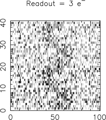
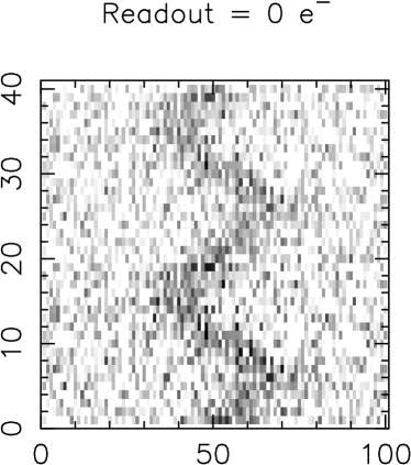
Figure 5: A simulation of the trailed spectrum of the $V=21$ ultra-compact binary star, RX J0806+1527, as taken with 1 night using the VLT and the FORS2 spectrograph (600 grism) with (left) and without (right) readout noise. Time advances upwards; the $x$-range is centred on a single emission line. The exposure time was taken to be 30 seconds in order to resolve the presumed 321 second orbital period of the object, but detector readout time was assumed to be zero in each case. The emission line was taken to be about as strong as seen in the average spectrum of Israel:RXJ0806

for a star of considerable current interest, RX J0806+1527. This is potentially the shortest period binary known, and a strong gravitational wave source, consisting of two white dwarfs with an orbital period of just $321$ seconds Ramsay:RXJ0806 ; Israel:RXJ0806 . This has yet to be proven however, and spectroscopy is by far the most promising avenue for testing it. It is however, as Fig. 5 shows, pushing the capabilities of even the VLT. The fact that as of mid-2006 this observation had yet to be performed is testament to its difficulty. Many would consider $V=21$ to be “bright”, or at least, not especially faint, but it certainly is when one is forced to take short exposures. Observations of this sort are exactly those needed for the gravitational wave sources, Sect. 2.3, except they will in general be more difficult still.

Having seen the limitations imposed by readout noise, I now turn to how it can potentially be avoided.

3.2 Electron-multiplying CCDs

The readout noise that so seriously limits normal CCDs is added by the amplifier which converts the small charge on each pixel into a voltage. To some extent readout noise can be reduced by taking longer over the double-correlated sampling used in low-noise CCD readouts (i.e. spending longer integrating the voltage levels before and after the charge on each pixel is cleared), but $1/f$ noise limits the extent to which one can push this and one cannot in any case take too long reading each pixel if one is interested in high speed. Electron-multiplying CCDs (hereafter EMCCDs, but also known as “low light level” or L3CCDs) get round this limitation in a clever way. In these CCDs, an extra series of stages is added to the serial register before the charge reaches the amplifier. These stages can be clocked with higher than normal voltages which creates a significant probability that one electron will generate another as the charges are moved from stage to stage. With enough stages, a single detected electron can lead to an avalanche of several hundred or even thousands of electrons. These then dwarf the readout noise added by the amplifier. The formulae for signal-to-noise from these devices are more complex than for standard CCDs Basden:L3CCD , but it is necessary to review them here in order to understand the advantages and limitations of these devices.

To first order, the avalanche gain register can be modelled as a series of stages at each of which there is a probability $p$ that any electron will spawn another. If there are $N$ such stages in total then the mean gain $g$, can be shown to be

$$g=(1+p)^{N}.$$ (7)

The value of $p$, and therefore $g$ is a parameter that can be controlled by adjustment of the driving voltages. For example if we take $N=536$ (appropriate to the CCD97 manufactured by the company, e2v) and $p=0.011$, then $g=352$. This gain is itself variable however (after it all it can in principle lie anywhere from 1 to $2^{N}\gg g$ although the extremes are unlikely) which increases the variance of the output over that expected from pure Poisson noise. Thus in a normal CCD readout, a mean detection rate of $C$ electrons leads to the variance contribution of $C$ in (4), while in an EMCCD the signal is amplified to $gC$ on average and the corresponding variance is $(g^{2}+\sigma^{2})C$ where $\sigma^{2}$ is the variance of the gain and is given by

$$\sigma^{2}=\frac{1-p}{1+p}\left(g^{2}-g\right).$$ (8)

Had there been no dispersion in the gain then the variance would have been $g^{2}C$, exactly what one would expect if simply multiplying $C$ by a constant; the variance in the gain thus adss extra noise. If, as is the case in practice, $p\ll 1$ and $g\gg 1$, then $\sigma^{2}\approx g^{2}$, and the variance is a factor of $2$ larger than a constant gain would have produced. Thus (4) is modified to

$$V=R^{2}+2g^{2}C,$$ (9)

and the signal-to-noise ratio for one pixel is given by

$$\frac{C}{\sqrt{(R/g)^{2}+2C}},$$ (10)

compared to

$$\frac{C}{\sqrt{R^{2}+C}},$$ (11)

for a normal CCD. The extra variance can be thought of as being equivalent to a 50% drop in QE. Put this way it sounds bad, but comparing the above two relations for signal-to-noise, and assuming that $g$ is so large that $R/g$ can be neglected, one can see that the EMCCD gains once $C<R^{2}$. In other words once $C\sim R^{2}$, normal CCDs have also effectively lost a factor 2 in QE, but unlike EMCCDs normal CCDs carry on getting worse as $C$ drops. This analysis also shows that (5) marks the dividing line between normal CCDs versus EMCCDs running in “linear” mode with counts proportional to the voltage of the amplifier.

At very low count rates, the full QE can be recovered by operating in a photon counting mode. In this case rather than take the output divided by the mean gain as an estimate of the counts, one defines a threshold $T$ such that an output $>T$ is recorded as one photon, while an output $<T$ is recorded as zero. Provided that one is operating in a regime where the chance of more than 1 e^-/pixel/exposure is small, this adds no extra noise to the output, and the signal-to-noise becomes

$$\frac{C}{\sqrt{(R/g)^{2}+C}}.$$ (12)

If $g$ is large, this implies ideal, Poisson-limited performance. Such a device could give us data looking like the right- rather than the left-hand side of Fig. 5.

Problems: thresholds, non-linearity and Clock-Induced Charges

EMCCDs suffer from some drawbacks, that apply to normal CCDs but which are not usually apparent above readout noise. First of all, given the variable gain, which can in principle be as low as $1$, a finite threshold must imply some loss of counts and therefore QE. To know how much, one needs to know the full probability distribution of the gain. For a single electron input, low $p$, high $g$ case, the output probability distribution function (PDF) for $n$ counts is quite well approximated by $g^{-1}\exp-n/g$ Basden:L3CCD . Figure 6

Figure 6: The solid line shows an exact computation of the output probability distribution function of a 536 stage electron multiplying register with $p=0.011$ given an input of 1 electron. The dashed line shows the approximation $\exp(-n/g)/g$ from Basden:L3CCD where $n$ is the number of counts and the mean gain $g=352$ in this case. The approximation only deviates significantly for values which are very rare

shows a comparison between an exact calculation of the PDF and this simple approximation, showing it to be good. This immediately implies that a threshold $T$ leads to a decrease in the QE by factor of $\exp(-T/g)$. One therefore wants $T\ll g$ to avoid too large a loss in QE, but at the same time $T$ must not be so low that readout noise alone leads to spurious counts, i.e. $T>4$ – $5$ times $R$, so that for gaussian noise there is a very small chance of counts induced artificially by readout noise.

The next problem is a common feature of photon counting devices, which is non-linearity at “high” count rates. In this case significant non-linearity will set in when the mean count rate rises above $\sim 0.2\,$e/pixel/exposure. Thus one can be limited by the rate at which pixels can be clocked out. This is exactly like the IPCS except that one can elect in the case of EMCCDs to work in the linear mode if it is clear that the count rates are too high for reliable photon counting.

The third and worst problem is a new phenomenon, or at least one that is only revealed by the low noise capabilities of EMCCDs: “Clock Induced Charges” or CICs. These are electrons which are spontaneously produced during clocking. Their statistics are complex and I leave a detailed discussion of them to the appendix where I include calculations that as far as I am aware have not been published before. As far as we are concerned they are equivalent to a readout noise and lead to a variance (in the photon counting case) of the form

$$V=\left(\frac{R}{g}\right)^{2}+R_{C}+C,$$ (13)

where $R_{C}$ is the number of CICs/pixel/exposure, equivalent to a readout noise before avalanche amplification of $R_{C}^{1/2}$. The $C$ here should be interpreted as including the $\exp(-T/g)$ factor discussed above, and the $R_{C}$ rate will similarly be threshold dependent in this case. The CICs are better thought of as a source of readout noise than background counts because they are incurred per exposure, not per unit time.

The three possible operating modes of CCDs are summarised in Fig. 7.

Figure 7: The three operating modes of CCDs are shown in terms of the exposure time taken to reach a given signal-to-noise compared to a “perfect” detector of identical QE. Normal mode (solid line) is best at high count levels drops off sharply once readout noise dominates. Photon counting mode (dot-dashed line) is best at very low count levels but cannot go past 1 e^-/pixel/exposure owing to non-linearity. In between, linear or “proportional” mode (dashed line) is best despite the 50% QE drop caused by the variable avalanche gain. The rise at very low counts is caused by CICs, with a rate of $0.01\,$e/pixel/exposure assumed here

For EMCCDs the focus is often on photon counting mode and the need to clock the pixels out fast to retain linearity. Figure 7 shows that there remains a role for the linear mode, the fraction of parameter space it occupies depending upon the CIC rate. Note that I have extended the regime of the linear mode in Fig. 7 towards lower counts than might seem justified by the curves; this is because of the non-linearity of photon counting. In principle it can be corrected to some extent, and this is built into Fig. 7, however in practice non-linearity corrections do not work as well as one might hope and I have restricted the photon counting mode to rates less than $0.3$ e^-/pixel/exposure.

Clearly the CIC rate is of central importance in how well these devices will perform in practice, as has been recognised before Daigle:L3CCD . Rates in the range $0.004$ to $0.1$ CICs/pixel/exposure have been quoted Tulloch:L3CCD . One can hope for manufacture-driven improvements with time, and controller improvements have a significant role to play too MacKay:L3CCD , but one should not lose sight of the fact that already even the high rate of $0.1$ CICs/pixel/exposure is equivalent to an extremely low readout noise and can allow the count rate $C$ to drop by a factor of 100 compared to normal CCDs before the noise floor is hit; this is an impressive potential gain and exactly what it needed to carry out high-time resolution spectroscopy on faint objects. Having said that, CICs do negate the QE advantages of CCDs compared to alternatives, in particular GaAs image intensifiers Daigle:L3CCD .

OPTICON-funded L3CCD for spectroscopy

Given the uncertainties over CIC rates, thresholds, pixel clocking rates and the like, EMCCDs are very much in the development phase for astronomy. We don’t yet know indeed whether they are reliable for spectroscopy in the sense that they can return accurate atomic line profiles, equivalent widths and radial velocities. Thus as part of the OPTICON programme of the EU’s Framework Programme 6 (FP6), the Universities of Sheffield and Warwick, and the Astronomy Technology Centre, Edinburgh have started a programme to characterise an EMCCD for spectroscopic work. We have purchased a CCD201 which is a frame transfer device with a 1k $\times$ 1k imaging area and with one normal and one avalanche readout. As of mid-2006, the device is mounted in a cryostat and producing test data. We will be using hardware developed for the high-speed camera ULTRACAM Dhillon:ULTRACAM . In terms of imaging area, this device is not competitive with existing detectors on spectrographs. On top of this the ULTRACAM controller will not push the device to its limits and so clear improvements are possible even now. However, it will allow us to see whether these devices are a promising route to explore for future development of high-speed spectroscopy.

4 Conclusion

High-speed optical spectroscopy offers a number of unique diagnostics of extreme astrophysical environments and will become only more necessary as larger surveys discover more unusual objects. Unfortunately standard CCDs, the workhorses of optical astronomy, are not well suited to the high-speed and low noise required when light is dispersed. This may be changing with recent developments of avalanche gain CCDs, but they must be tested on celestial objects before we know whether this is truly the case. This is the aim of a programme funded under the EU FP6’s OPTICON consortium.

5 Clock Induced Charge statistics

In this section we detail some of the statistical properties of CICs. CICs come in two varieties: “pre-register” and “in-register” events. Pre-register events suffer the full amplification of the avalanche stage and will have identical statistics to electrons generated from genuine signals. In-register events are amplified by a variable amount depending upon where in the avalanche register they are first produced. This leads to an extremely skewed distribution for these events with lots of low values but a tail extending to very high values as well as shown in Fig. 8.

Figure 8: In the left panel the solid line shows the distribution of in-register CICs for a 536 stage electron multiplying register with $p=0.011$ and CIC probability/stage of $p_{c}=0.0011$, i.e. this is the output PDF given a zero electron input. The dashed line shows the PDF given an input of 1 electron with $p_{c}$ set to zero. The right-hand panel shows the equivalent cumulative distribution functions, and illustrates that the parameters chosen here will give a CIC above 100 counts in about 1 in 10 pixels

The skewed distribution makes it hard to define CIC rates in a general way. For example, Fig. 8 shows that for the particular parameters chosen about 25% of pre-register CICs would on output fall below a threshold of 100, while 90% of the in-register CICs will do so. Lowering the threshold could increase the pre-register rate by at most 25%, but could increase the in-register rate by up to 10 times. When quoting rates, it is important to define how they were measured. In this case a threshold of 100 will lead to a rate of $0.1$ CIC/pixel/exposure, at the high end of total CIC rates (in- plus pre-register) [40], and so presumably the probability of a CIC being generated at any one stage of the avalanche register is usually less than I have assumed.

If the probability of a CIC being generated at any one stage of the avalanche register is $p_{C}$, then one can show that the mean output value, given zero input $\mu_{C}$ is given by

$$\mu_{C}=\frac{p_{C}}{p}(g-1),$$ (14)

while the variance is

$$\sigma^{2}_{C}=\left(\frac{2/(1+p)-p_{c}}{2+p}(g+1)-\frac{1-p}{1+p}\right)\mu_{C}.$$ (15)

For $p\ll 1$, $p_{C}\ll 1$, $g\gg 1$, this boils down to $V_{C}\approx g\mu_{C}$. For the example shown in Fig. 8, $\mu_{C}=35$ while $\sigma_{C}=110$. In proportional mode, this is effectively equivalent to a readout noise component of $R=\sigma_{C}/g=0.3$ entering the variance equation $V=R^{2}+2C$ (ignoring the amplifier readout noise). A threshold of 100 leads to a very similar number for photon counting mode.

There may be some room for optimisation of the threshold in the presence of significant numbers of in-register CICs. In the example shown, a threshold of 100 leads to a 25% reduction in the true event rate and a 10% CIC rate, so that the signal-to-noise would be

$$\frac{0.75P}{\sqrt{0.1+0.75P}},$$ (16)

where $P$ is the mean number of photo-electrons per pixel per exposure. If the threshold is raised to 200, this becomes

$$\frac{0.57P}{\sqrt{0.05+0.57P}},$$ (17)

which is better for $P<0.057$.

The threshold cannot be optimised for pre-register events in the same way since they have identical statistics to genuine events. The relative numbers of in-register and pre-register events appears to depend upon the controller [40, 20]. My suspicion, which is possibly borne out by one of these studies [20], would be that the high voltages required for the avalanche register will make it harder to reduce the in-register compared to pre-register event rates.

References

- [1] A. G. Basden, C. A. Haniff, and C. D. Mackay. Photon counting strategies with low-light-level CCDs. MNRAS, 345:985–991, November 2003.
- [2] A. Boksenberg. UCL Image Photon Counting System. In Auxiliary Instrumentation for Large Telescopes, Proc. of the ESO-CERN Conference, ed. S.Lausten, A.Reiz, page 295, 1972.
- [3] A. Bragaglia, L. Greggio, A. Renzini, and S. D’Odorico. Double degenerates among da white dwarfs. ApJL, 365:L13–L17, December 1990.
- [4] P. Brassard, G. Fontaine, M. Billères, S. Charpinet, J. Liebert, and R. A. Saffer. Discovery and Asteroseismological Analysis of the Pulsating sdB Star PG 0014+067. ApJ, 563:1013–1030, December 2001.
- [5] C. S. Brinkworth, T. R. Marsh, V. S. Dhillon, and C. Knigge. Detection of a period decrease in NN Ser with ULTRACAM: evidence for strong magnetic braking or an unseen companion. MNRAS, 365:287–295, January 2006.
- [6] J. Casares, T. Muñoz-Darias, I. G. Martínez-Pais, R. Cornelisse, P. A. Charles, T. R. Marsh, V. S. Dhillon, and D. Steeghs. Echo Tomography of Sco X-1 using Bowen Fluorescence Lines. In L. Burderi, L. A. Antonelli, F. D’Antona, T. di Salvo, G. L. Israel, L. Piersanti, A. Tornambè, and O. Straniero, editors, AIP Conf. Proc. 797: Interacting Binaries: Accretion, Evolution, and Outcomes, pages 365–370, October 2005.
- [7] S. Charpinet, G. Fontaine, P. Brassard, M. Billères, E. M. Green, and P. Chayer. Structural parameters of the hot pulsating B subdwarf Feige 48 from asteroseismology. A&A, 443:251–269, November 2005.
- [8] S. Charpinet, G. Fontaine, P. Brassard, E. M. Green, and P. Chayer. Structural parameters of the hot pulsating B subdwarf PG 1219+534 from asteroseismology. A&A, 437:575–597, July 2005.
- [9] J. C. Clemens, M. H. van Kerkwijk, and Y. Wu. Mode identification from time-resolved spectroscopy of the pulsating white dwarf G29-38. MNRAS, 314:220–228, May 2000.
- [10] A. Cooray, A. J. Farmer, and N. Seto. The Optical Identification of Close White Dwarf Binaries in the Laser Interferometer Space Antenna Era. ApJL, 601:L47–L50, January 2004.
- [11] O. Daigle, J.-L. Gach, C. Guillaume, C. Carignan, P. Balard, and O. Boisin. L3CCD results in pure photon-counting mode. In J. D. Garnett and J. W. Beletic, editors, Optical and Infrared Detectors for Astronomy. Edited by James D. Garnett and James W. Beletic. Proceedings of the SPIE, Volume 5499, pp. 219-227 (2004)., pages 219–227, September 2004.
- [12] V. Dhillon and T. Marsh. ULTRACAM - studying astrophysics on the fastest timescales. New Astronomy Review, 45:91–95, January 2001.
- [13] S. Falter, U. Heber, S. Dreizler, S. L. Schuh, O. Cordes, and H. Edelmann. Simultaneous time-series spectroscopy and multi-band photometry of the sdBV PG 1605+072. A&A, 401:289–296, April 2003.
- [14] P. J. Groot. Evolution of Spiral Shocks in U Geminorum during Outburst. ApJL, 551:L89–L92, April 2001.
- [15] D. Hils, P. L. Bender, and R. F. Webbink. Gravitational radiation from the galaxy. ApJ, 360:75–94, September 1990.
- [16] K. Horne. An optimal extraction algorithm for CCD spectroscopy. PASP, 98:609–617, June 1986.
- [17] K. Horne and T. R. Marsh. Emission line formation in accretion discs. MNRAS, 218:761–773, February 1986.
- [18] R. Ishioka, S. Mineshige, T. Kato, D. Nogami, and M. Uemura. Line-Profile Variations during an Eclipse of a Dwarf Nova, IP Pegasi. PASJ, 56:481–485, June 2004.
- [19] G. L. Israel, W. Hummel, S. Covino, S. Campana, I. Appenzeller, W. Gässler, K.-H. Mantel, G. Marconi, C. W. Mauche, U. Munari, I. Negueruela, H. Nicklas, G. Rupprecht, R. L. Smart, O. Stahl, and L. Stella. RX J0806.3+1527: A double degenerate binary with the shortest known orbital period (321s). A&A, 386:L13–L17, May 2002.
- [20] C. Mackay, A. Basden, and M. Bridgeland. Astronomical imaging with L3CCDs: detector performance and high-speed controller design. In J. D. Garnett and J. W. Beletic, editors, Optical and Infrared Detectors for Astronomy. Edited by James D. Garnett and James W. Beletic. Proceedings of the SPIE, Volume 5499, pp. 203-209 (2004)., pages 203–209, September 2004.
- [21] T. R. Marsh. The extraction of highly distorted spectra. PASP, 101:1032–1037, November 1989.
- [22] T. R. Marsh. Doppler Tomography. LNP Vol. 573: Astrotomography, Indirect Imaging Methods in Observational Astronomy, pages 1–26, 2001.
- [23] T. R. Marsh, V. S. Dhillon, and S. R. Duck. Low-Mass White Dwarfs Need Friends - Five New Double-Degenerate Close Binary Stars. MNRAS, 275:828–+, August 1995.
- [24] T. R. Marsh and K. Horne. Images of accretion discs. ii - doppler tomography. MNRAS, 235:269–286, November 1988.
- [25] T. R. Marsh, G. Nelemans, and D. Steeghs. Mass transfer between double white dwarfs. MNRAS, 350:113–128, May 2004.
- [26] P. F. L. Maxted, T. R. Marsh, and C. K. J. Moran. The mass ratio distribution of short-period double degenerate stars. MNRAS, 332:745–753, May 2002.
- [27] C. Moran, T. R. Marsh, and A. Bragaglia. A detached double degenerate with a 1.4-h orbital period. MNRAS, 288:538–544, June 1997.
- [28] C. Motch, S. A. Ilovaisky, and C. Chevalier. Discovery of fast optical activity in the X-ray source GX 339-4. A&A, 109:L1–L4, May 1982.
- [29] R. Napiwotzki, L. Yungelson, G. Nelemans, T. R. Marsh, B. Leibundgut, R. Renzini, D. Homeier, D. Koester, S. Moehler, N. Christlieb, D. Reimers, H. Drechsel, U. Heber, C. Karl, and E.-M. Pauli. Double degenerates and progenitors of supernovae type Ia. In ASP Conf. Ser. 318: Spectroscopically and Spatially Resolving the Components of the Close Binary Stars, pages 402–410, November 2004.
- [30] R. E. Nather and B. Warner. Observations of rapid blue variables. I. Techniques. MNRAS, 152:209, 1971.
- [31] G. Nelemans, L. R. Yungelson, and S. F. Portegies Zwart. The gravitational wave signal from the Galactic disk population of binaries containing two compact objects. A&A, 375:890–898, September 2001.
- [32] G. Nelemans, L. R. Yungelson, and S. F Portegies Zwart. Short-period AM CVn systems as optical, X-ray and gravitational-wave sources. MNRAS, 349:181–192, March 2004.
- [33] G. Ramsay, P. Hakala, and M. Cropper. RX J0806+15: the shortest period binary? MNRAS, 332:L7–L10, May 2002.
- [34] E. L. Robinson, T. M. Mailloux, E. Zhang, D. Koester, R. F. Stiening, R. C. Bless, J. W. Percival, M. J. Taylor, and G. W. van Citters. The pulsation index, effective temperature, and thickness of the hydrogen layer in the pulsating DA white dwarf G117-B15A. ApJ, 438:908–916, January 1995.
- [35] A. D. Schwope, K. H. Mantel, and K. Horne. Phase-resolved high-resolution spectrophotometry of the eclipsing polar hu aquarii. A&A, 319:894–908, March 1997.
- [36] D. Steeghs and J. Casares. The Mass Donor of Scorpius X-1 Revealed. ApJ, 568:273–278, March 2002.
- [37] D. Steeghs, E. T. Harlaftis, and K. Horne. Spiral structure in the accretion disc of the binary IP Pegasi. MNRAS, 290:L28–L32, September 1997.
- [38] D. Steeghs, K. O’Brien, K. Horne, R. Gomer, and J. B. Oke. Emission-line oscillations in the dwarf nova V2051 Ophiuchi. MNRAS, 323:484–496, May 2001.
- [39] A. Stroeer, A. Vecchio, and G. Nelemans. LISA Astronomy of Double White Dwarf Binary Systems. ApJL, 633:L33–L36, November 2005.
- [40] S. M. Tulloch. Photon counting and fast photometry with L3 CCDs. In A. F. M. Moorwood and M. Iye, editors, Ground-based Instrumentation for Astronomy. Edited by Alan F. M. Moorwood and Iye Masanori. Proceedings of the SPIE, Volume 5492, pp. 604-614 (2004)., pages 604–614, September 2004.
- [41] M. H. van Kerkwijk, J. C. Clemens, and Y. Wu. Surface motion in the pulsating DA white dwarf G29-38. MNRAS, 314:209–219, May 2000.