Topology of the regular part for infinitely renormalizable quadratic polynomials

Abstract

In this paper we describe the well studied process of renormalization of quadratic polynomials from the point of view of their natural extensions. In particular, we describe the topology of the inverse limit of infinitely renormalizable quadratic polynomials and prove that when they satisfy a-priori bounds, the topology is rigid modulo its combinatorics.

1 Introduction and basic theory

The last quarter of the last century witnessed an explosion of results concerning the quadratic family. Of particular importance was the development of the notion of renormalization which allowed to describe much of the dynamical richness the family posses. In this setting, important contributions were given by the work of several people: Feigenbaum, Douady, Hubbard, Sullivan, Yoccoz, Lyubich and McMullen among many others.

In [20], Sullivan constructed a lamination by Riemann surfaces associated to expanding maps on the circle, by using its inverse limit. Later on in [16], Lyubich and Minsky generalized this construction to every rational map on the sphere. In this setting the construction of the lamination is more involved since the presence of critical orbits forces to consider a subset of the inverse limit, called the regular space, provided with a finer topology than the induced from the product topology on the inverse limit.

Part of the program presented by Lyubich and Minsky, it was to investigate the properties of the regular part for infinite renormalizable polynomials.

Under the assumption of a-priori bounds, the regular part of an infinite renormalizable polynomial $f_{c}$ is a lamination under the topology induced from its inverse limit.

In this paper, we show that the topology of the regular part determines the dynamics of $f_{c}$ up to combinatorial equivalence (Main Theorem). This implies a kind of rigidity of the regular parts associated with infinitely renormalizable maps with a priori bounds.

Outline of this paper. In the rest of this section we give the basic theory of the dynamics of quadratic maps and their renormalizations. In Section 2, we review the definition of the inverse limits and the regular parts generated by quadratic maps. Section 3 is devoted for the statement and the proof of the Structure Theorem (Theorem 4), which claims that regular parts of the persistently recurrent infinitely renormalizable maps are decomposed into “blocks” according to the tree structure associated with the nest of renormalizations. Finally in Section 4, we prove the Main Theorem (Theorem 7) stated as above.

Acknowledgements. We would like to thank for their hospitality and support to the Fields institute and IMPAN (Warsaw) were this work was carried on. We would also want to thank Misha Lyubich for useful conversations. The first author want to thank for the hospitality and support of IMATE (Cuernavaca). The second author is partially supported by JSPS Grant-in-Aid for Young Scientists, the Circle for the Promotion of Science and Engineering, and Inamori Foundation.

1.1 Preliminary

We start with some basic definitions on the dynamics of quadratic maps and inverse limits. Readers may refer [4] and [13] for dynamics of quadratic maps.

Julia and Fatou sets. For quadratic map $f_{c}(z)=z^{2}+c$ on the Riemann sphere $\overline{\mathbb{C}}$ with parameter $c\in\mathbb{C}$, the Julia set $J(f_{c})$ is defined as the closure of the repelling periodic points of $f_{c}$. Its complement $F(f_{c})=\mathbb{C}-J(f_{c})$ is called the Fatou set. The set $K(f_{c})$ of points with bounded orbit is called the filled Julia set. It is known that the boundary $\partial K(f_{c})$ coincides with $J(f_{c})$, and that $K(f_{c})$ and $J(f_{c})$ are either both connected or the same Cantor set.

Böttcher coordinates, equipotentials, external rays. Throughout this paper we assume that $K(f_{c})$ and $J(f_{c})$ are both connected. In this case, the set $A_{c}:=\overline{\mathbb{C}}-K(f_{c})$ is a simply connected region which consists of points whose orbits tend to infinity. We call $A_{c}$ the basin of infinity of $f_{c}$. There exists a unique Riemann map $\psi_{c}:A_{c}\rightarrow\overline{\mathbb{C}}-\overline{\mathbb{D}}$, called the Böttcher coordinate, that conjugates $f_{c}$ in $A_{c}$ with $w\mapsto w^{2}$ on $\overline{\mathbb{C}}-\overline{\mathbb{D}}$ and $\psi_{c}(z)/z\to 1~{}(z\to\infty)$. For $r>1$, $E_{c}(r):=\psi_{c}^{-1}({\left\{w\in\mathbb{C}\,:\,|w|=r\right\}})$ is called the equipotential curve of level $r$. For $\theta\in\mathbb{R}/\mathbb{Z}$, $R_{c}(\theta):=\psi_{c}^{-1}({\left\{w\in\mathbb{C}-\overline{\mathbb{D}}\,:\,\arg w=\theta\right\}})$ is called the external ray of angle $\theta$.

Ray portrait. Let $O={\left\{p_{1},\ldots,p_{m}\right\}}$ be a repelling cycle of $f_{c}$. There are finitely many angles of external rays landing at each $p_{i}$, which we denote by $\Theta(p_{i})$. It is a fact due to Douady and Hubbard [4] that $\Theta(p_{i})$ is a set of rational numbers. The collection $\mathrm{rp}(O)=\{\Theta(p_{1}),\ldots,\Theta(p_{m})\}$ is called the ray portrait of $O$. A ray portrait is called non trivial, if there are at least two rays landing at every point in $O$. A non trivial ray portrait determines a region in the parameter space with a leading hyperbolic component. In this way, every non trivial ray portrait determines a unique superattracting parameter by taking the center of its leading hyperbolic component. (See Milnor’s [19])

Superattracting quadratic maps. Quadratic maps $f_{s}(z)=z^{2}+s$ whose critical orbit is periodic form an important class of quadratic maps, called superattracting quadratic maps. Let ${\left\{{\alpha}_{s}(1),\ldots,{\alpha}_{s}(m)=0\right\}}$ denote the critical cycle with $f_{s}({\alpha}_{s}(i))={\alpha}_{s}(i+1)$, where we take the indexes modulo $m$. Then it is known that the connected component $D_{s}$ of the Fatou set (“Fatou component”) with ${\alpha}_{s}(m)=0\in D_{s}$ is a Jordan domain with dynamics $f_{s}^{m}:\bar{D_{s}}\to\bar{D_{s}}$ conjugate to $f_{0}:\overline{\mathbb{D}}\to\overline{\mathbb{D}}$. Let $\Psi_{s}:\bar{D_{s}}\to\overline{\mathbb{D}}$ be this conjugacy, which we also call a Böttcher coordinate for $\bar{D_{s}}$. The internal equipotential $I_{s}(r)$ of level $r<1$ is defined by $\Psi_{s}^{-1}({\left\{|w|=r\right\}})$. We also denote $\Psi_{s}^{-1}({\left\{|w|<r\right\}})$ by $D_{s}(r)$.

The pull-back of $1\in\overline{\mathbb{D}}$ by $\Psi_{s}$ in $\partial D_{s}$ is a repelling periodic point with period $\leq m$. Let $O_{s}$ be its cycle which is on the boundary of $\bigcup_{1\leq i\leq m}f_{s}^{i}(D_{s})$. We say the ray portrait $\mathrm{rp}(O_{s})$ is the characteristic ray portrait of $f_{s}$. In fact, superattracting $f_{s}$ is uniquely identified by $\mathrm{rp}(O_{s})$. (See Milnor’s [19]).

Quadratic-like maps. Let $U$ and $V$ be topological disks in $\mathbb{C}$ with $U$ compactly contained in $V$. A quadratic-like map $g:U\to V$ is a proper holomorphic map of degree two. The filled Julia set is defined by $K(g):=\bigcap_{n\geq 1}g^{-n}(V)$. Throughout this paper we assume that any quadratic-like map $g:U\to V$ has a connected $K(g)$. Its Julia set $J(g)$ is the boundary of $K(g)$. The postcritical set $P(g)$ is the closure of the forward orbit of the critical point of $g$, since $K(g)$ is connected we have $P(g)\subset U$.

By the Douady-Hubbard straightening theorem [4], there exists a unique $c=c(g)\in\mathbb{C}$ and a quasiconformal map $h:V\to V^{\prime}$ such that $h$ conjugates $g:U\to V$ to $f_{c}:U^{\prime}\to V^{\prime}$ where $U^{\prime}=h(U)={f_{c}}^{-1}(V^{\prime})$ and $\bar{\partial}h=0$ a.e. on $K(g)$. The quadratic map $f_{c}$ is called the straightening of $g$ and $h$ is called a straightening map. Though such an $h$ is not uniquely determined, we always assume that any quadratic-like map $g$ is accompanied by one fixed straightening map $h=h_{g}$.

One can easily check that there exists an $r_{g}>1$ such that if $1<r\leq r_{g}$ and $\theta\in\mathbb{R}/\mathbb{Z}$, the pulled-back equipotentials and external rays

$$E_{g}(r)~{}:=~{}h^{-1}(E_{c}(r))~{}~{}\text{and}~{}~{}R_{g}(\theta)~{}:=~{}h^{-1}({\left\{\rho e^{2\pi i\theta}\,:\,1<\rho\leq r_{g}\right\}})$$

are defined. For the straightening $f_{c}$ of $g$, there exists a repelling or parabolic fixed point $\beta(f_{c})\in K(f_{c})$ which is the landing point of the external ray $R_{c}(0)$. Note that $\beta(f_{c})$ is repelling unless $c=1/4$. We set $\beta(g):=h^{-1}(\beta({f_{c}}))$ and call it the $\beta$-fixed point of $g$.

Renormalization of quadratic maps A quadratic-like map $g:U\rightarrow V$ is said to be renormalizable, if there exist a number $m>1$, called the order of renormalization, and two open sets $U_{1}\subset U$ and $V_{1}\subset V$ containing the critical point of $g$, such that $g_{1}=g^{m}|~{}U_{1}\rightarrow V_{1}$, called a pre-renormalization of $g$, is again a quadratic-like map with connected Julia set $K(g_{1})$. We say $g_{1}:U_{1}\rightarrow V_{1}$ is a renormalization of $g:U\to V$. We call $K_{1}:=K(g_{1})$, $g(K_{1})$, $\cdots$, $g^{m-1}(K_{1})$ the little Julia sets. We also assume that $m$ is the minimal order with this property and that $K_{1}$ has the following property: For any $1\leq i<j\leq m$, $g^{i}(K_{1})\cap g^{j}(K_{1})$ is empty or just one point that separates neither $g^{i}(K_{1})$ nor $g^{j}(K_{1})$. Such a renormalization is called simple or non-crossing. See [17] or [18] for examples of crossing renormalizations.

Infinitely renormalizable maps. In this paper we only deal with quadratic-like maps which are restrictions of some iterated quadratic map. For any quadratic map $f_{c}$ and any $r>1$, $f_{c}|~{}U_{c}(r)\mapsto U_{c}(r^{2})$ is a quadratic map. Set $g_{0}=f_{c}$, $U_{0}:=U_{c}(r)$ and $V_{0}:=U_{c}(r^{2})$. We say $f_{c}$ is infinitely renormalizable if there is an infinite sequence of numbers $p_{0}=1<p_{1}<p_{2}<\cdots$ and two sequences of open sets $\{U_{n}\}$ and $\{V_{n}\}$ such that each $g_{n}=f_{c}^{p_{n}}:U_{n}\to V_{n}$ is a quadratic-like map, with the property that $g_{n+1}$ is a pre-renormalization of $g_{n}$ of order $m_{n}:=p_{n+1}/p_{n}>1$. See [15] for more details. The index $n$ of $g_{n}$ is called the level of renormalization.

Combinatorics of renormalizable maps. For a complete exposition of combinatorics of renormalizable maps we refer to the work of Lyubich in [14] and [15]. From now on $f_{c}$ will denote an infinitely renormalizable quadratic map and ${\left\{g_{n}:U_{n}\to V_{n}\right\}}$ be its associated sequence of quadratic-like maps as above. In order to describe the combinatorics of $f_{c}$, first we observe that the orbit of the $\beta$-fixed point of $g_{n+1}$ forms a repelling cycle $O_{n}$ of $g_{n}$. Since every $g_{n}$ has a unique straightening $f_{c_{n}}$ with $c_{n}=c(g_{n})$ by the straightening map $h_{n}$, $h_{n}(O_{n})$ is also a repelling cycle of $f_{c_{n}}$ with at least 2 external rays landing at each point in $h_{n}(O_{n})$, hence its ray portrait $\mathrm{rp}(h_{n}(O_{n}))$ is non-trivial. Since every non-trivial ray portrait determines a unique superattracting quadratic map, the $n$-level of renormalization induces a unique superattracting map $f_{s_{n}}(z)=z^{2}+s_{n}$ with characteristic ray portrait $\mathrm{rp}(h_{n}(O_{n}))$. We call the infinite sequence of superattracting parameters $\{s_{0},s_{1},s_{2},\ldots\}$ the combinatorics of $f_{c}$, note that the period of the critical point of $f_{s_{n}}$ is equal to $m_{n}$.

We say that $f_{c}$ has bounded combinatorics if the sequence $\{m_{n}\}$ is bounded. The polynomial $f_{c}$ is said to have a-priori bounds if there exist $\epsilon>0$, independent of $n$, such that $mod(V_{n}\setminus U_{n})>\epsilon$. The map $f_{c}$ is called Feigenbaum if it has a priori bounds and bounded combinatorics.

2 Inverse limits and regular parts

In the theory of dynamical systems we use the technique of the inverse limit to construct an invertible dynamics out of non-invertible dynamics. In this section we give some inverse limits associated with quadratic dynamics used in this paper. We also define the regular parts, which is analytically well-behaved parts of the inverse limits, according to [16]. Readers may refer [16] and [8] where more details on the objects defined here are given.

2.1 Inverse limits and solenoidal cones

Inverse Limits. Consider $\{f_{-n}:X_{-n}\rightarrow X_{-n+1}\}_{n=1}^{\infty}$, a sequence of $d$-to-$1$ branched covering maps on the manifolds $X_{-n}$ with the same dimension. The inverse limit of this sequence is defined as

$$\underset{\longleftarrow}{\lim}(f_{-n},X_{-n})~{}:=~{}\{\hat{x}=(x_{0},x_{-1},x_{-2}\ldots)\in\prod_{n\geq 0}X_{-n}\,:\,f_{-n}(x_{-n})=x_{-n+1}\}.$$

The space $\underset{\longleftarrow}{\lim}(f_{-n},X_{-n})$ has a natural topology which is induced from the product topology in $\prod X_{-n}$. The projection $\pi:\underset{\longleftarrow}{\lim}(f_{-n},X_{-n})\to X_{0}$ is defined by $\pi(\hat{x}):=x_{0}$.

Example 1: Natural extensions of quadratic maps. When all the pairs $(f_{-n},X_{-n})$ coincide with the quadratic $(f_{c},\overline{\mathbb{C}})$, following Lyubich and Minsky [16], we will denote $\underset{\longleftarrow}{\lim}(f_{c},\bar{\mathbb{C}})$ by $\mathcal{N}_{c}$. The set $\mathcal{N}_{c}$ is called the natural extension of $f_{c}$. In this case we denote the projection by $\pi_{c}:\mathcal{N}_{c}\to\overline{\mathbb{C}}$. There is a natural homeomorphic action $\hat{f}_{c}:\mathcal{N}_{c}\to\mathcal{N}_{c}$ given by $\hat{f}_{c}(z_{0},z_{-1},\ldots):=(f_{c}(z_{0}),z_{0},z_{-1},\ldots)$.

Let $X$ be a forward invariant set, by $\hat{X}$ we will denote the invariant lift of $X$, that is the set of $\hat{z}\in\mathcal{N}_{c}$ such that all coordinates of $\hat{z}$ belong to $X$. In particular, $\hat{\infty}=(\infty,\infty,\ldots)$.

The natural extension is not so artificial than it appears. For example, it is known that if $f_{c}$ is hyperbolic, then $\hat{f}_{c}$ acting on $\mathcal{N}_{c}-{\left\{\hat{\infty}\right\}}$ is topologically conjugate to a Hénon map of the form $(z,w)\mapsto(z^{2}+c-aw,z)$ with $|a|\ll 1$ acting on the backward Julia set $J^{-}$. See [5] for more details.

Example 2: Dyadic solenoid and solenoidal cones. A well-known example of an inverse limit is the dyadic solenoid $\mathcal{S}^{1}:=\underset{\longleftarrow}{\lim}(f_{0},\mathbb{S}^{1})$, where $f_{0}(z)=z^{2}$ and $\mathbb{S}^{1}$ is the unit circle in $\mathbb{C}$. The dyadic solenoid is a connected set but is not path-connected. Any space homeomorphic to $\underset{\longleftarrow}{\lim}(f_{0},\overline{\mathbb{C}}-\overline{\mathbb{D}})$ will be called a solenoidal cone. For $f_{c}$ with connected $K(f_{c})$, we have an important example of a solenoidal cone $\hat{A}_{c}:=\underset{\longleftarrow}{\lim}(f_{c},A_{c})$ in $\mathcal{N}_{c}$ by looking at $\underset{\longleftarrow}{\lim}(f_{0},\overline{\mathbb{C}}-\overline{\mathbb{D}})$ through the inverse Böttcher coordinate $\psi_{c}^{-1}$. More precisely, the set $\hat{A}_{c}$ is given by $\hat{\psi}_{c}^{-1}(\underset{\longleftarrow}{\lim}(f_{0},\overline{\mathbb{C}}-\overline{\mathbb{D}}))$ where $\hat{\psi}_{c}^{-1}:(z_{0},z_{-1},\ldots)\mapsto(\psi_{c}^{-1}(z_{0}),\psi_{c}^{-1}(z_{-1}),\ldots).$ Then $\hat{A}_{c}-\{\hat{\infty}\}$ is foliated by sets of the form $\mathcal{S}_{r}:=\pi_{c}^{-1}(E_{c}(r))$ with $r>1$. Each of $\mathcal{\pi}_{c}^{-1}(E_{c}(r))$ is homeomorphic to the dyadic solenoid; in fact, the map $\phi_{r}:\mathcal{S}_{r}\rightarrow\mathcal{S}^{1}$ given by $\phi_{r}:(z_{0},z_{1},...)\mapsto(z_{0}/r,z_{1}/r^{1/2},...)$ is a canonical homeomorphism. We call such $\mathcal{S}_{r}$ a solenoidal equipotential.

Let us give a few more examples of solenoidal cones. For any $r>1$, set $\mathbb{D}_{r}:={\left\{|z|<r\right\}}$. We denote the inverse limits associated with the backward dynamics

$$\cdots~{}\rightarrow~{}\overline{\mathbb{C}}-f_{0}^{-2}(\overline{\mathbb{D}}_{r})~{}\rightarrow~{}\overline{\mathbb{C}}-f_{0}^{-1}(\overline{\mathbb{D}}_{r})~{}\rightarrow~{}\overline{\mathbb{C}}-\overline{\mathbb{D}}_{r}$$

of $f_{0}(z)=z^{2}$ by $\hat{A}_{0}(r)$. This is a sub-solenoidal cone compactly contained in $\hat{A}_{0}\subset\mathcal{N}_{0}$. Similarly, we have a sub-solenoidal cone of $\hat{A}_{c}\subset\mathcal{N}_{c}$ given by $\hat{A}_{c}(r):=\hat{\psi}_{c}^{-1}(\hat{A}_{0}(r))$. Note that the boundary of $\hat{A}_{c}(r)$ in $\mathcal{N}_{c}$ is $\mathcal{S}_{r}$. We call the union $\hat{A}_{c}(r)\cup\mathcal{S}_{r}$ a compact solenoidal cone at infinity.

Let $f_{s}$ be a superattracting quadratic map as in the preceding section. For all $r<1$, the inverse limit given by the backward dynamics

$$\cdots~{}\rightarrow~{}D_{s}(r^{1/4})~{}\rightarrow~{}D_{s}(r^{1/2})~{}\rightarrow~{}D_{s}(r)$$

of $f_{s}^{m}$ is also a solenoidal cone. We denote it by $\underset{\longleftarrow}{\lim}(f_{s}^{m},D_{s}(r))$. We may consider $\underset{\longleftarrow}{\lim}(f_{s}^{m},D_{s}(r))$ as a subset of $\mathcal{N}_{s}$ by the following embedding map: For $(x_{0},x_{-1},\ldots)\in\underset{\longleftarrow}{\lim}(f_{s}^{m},D_{s}(r))$, we define $\iota:(x_{0},x_{-1},\ldots)\mapsto(y_{0},y_{-1},\ldots)\in\mathcal{N}_{s}$ so that $x_{-k}=y_{-mk}$ for all $k\geq 0$. Then $\hat{D_{s}}(r):=\iota(\underset{\longleftarrow}{\lim}(f_{s}^{m},D_{s}(r)))$ is a solenoidal cone in $\mathcal{N}_{s}$. Note that $\partial\hat{D_{s}}(r)$ is a proper subset of $\pi_{s}^{-1}(I_{s}(r))$ unless $s=0$. Now $\hat{D}_{s}(r)$, $\hat{f}_{s}(\hat{D}_{s}(r))$, $\ldots$, $\hat{f}_{s}^{m-1}(\hat{D}_{s}(r))$ are disjoint solenoidal cones in $\mathcal{N}_{s}$. We also call the closures of these $m$ solenoidal cones in $\mathcal{N}_{s}$ compact solenoidal cones at the critical orbit.

Quadratic-like inverse limits. Let $g:U\rightarrow V$ be a proper holomorphic map, we might allow here $U=V$, by $\underset{\longleftarrow}{\lim}(g,V)$ we denote the inverse limit for the sequence

$$\cdots~{}\rightarrow~{}g^{-2}(V)~{}\rightarrow~{}g^{-1}(V)~{}\rightarrow~{}V$$

Let us remark that even in the cases where $g$ is defined outside $U$, when taking preimages we will take all branches of the inverse of $g$ satisfying $g^{-n}(V)\subset U$.

Here we show the following fact on the relation between inverse limits of quadratic-like maps and its straightening:

Proposition 1.

Let $g:U\to V$ be a quadratic-like map with straightening $f_{c}(z)=z^{2}+c$. Then the inverse limit $\underset{\longleftarrow}{\lim}(g,V)$ is homeomorphic to $\mathcal{N}_{c}$ with a compact solenoidal cone at infinity removed.

Proof. Set

$$U_{g}(r)~{}:=~{}K(g)\cup\bigcup_{1<\rho<r}E_{g}(\rho)~{}~{}\text{and}~{}~{}U_{c}(r)~{}:=~{}K({f_{c}})\cup\bigcup_{1<\rho<r}E_{c}(\rho)$$

for $1<r<r_{g}$. Then $U_{g}(r)\Subset V$ and $g:U_{g}(\sqrt{r})\to U_{g}(r)$ is a quadratic-like map which is quasiconformally conjugate to ${f_{c}}:U_{c}(\sqrt{r})\to U_{c}(r)$ by straightening map $h$. Thus $\underset{\longleftarrow}{\lim}(g,U_{g}(r))$ is homeomorphic to $\underset{\longleftarrow}{\lim}({f_{c}},U_{c}(r))$, which is $\mathcal{N}_{c}$ with a compact solenoidal cone $\overline{\hat{A}_{c}(r)}$ removed.

Now it is enough to check that the original $\underset{\longleftarrow}{\lim}(g,V)$ is homeomorphic to its subset $\underset{\longleftarrow}{\lim}(g,U_{g}(r))$. But this follows from the fact that $g:U-U_{g}(\sqrt{r})\to V-U_{g}(r)$ is a double covering between annuli and $\underset{\longleftarrow}{\lim}(g,V)-\underset{\longleftarrow}{\lim}(g,U_{g}(r))$ is homotopic to the boundary of $\underset{\longleftarrow}{\lim}(g,U_{g}(r))$. $\blacksquare$

Remark. In fact, the homeomorphism is given by a leafwise quasiconformal map on their regular parts.

2.2 Regular parts and infinitely renormalizable maps

Regular parts of quadratic natural extensions. Let $f_{c}$ be a quadratic map. A point $\hat{z}=(z_{0},z_{-1},\ldots)$ in the natural extension $\mathcal{N}_{c}=\underset{\longleftarrow}{\lim}(f_{c},\overline{\mathbb{C}})$ is regular if there is a neighborhood $U_{0}$ of $z_{0}$ such that the pull-back of $U_{0}$ along $\hat{z}$ is eventually univalent. The regular part(or regular leaf space) $\mathcal{R}_{f_{c}}=\mathcal{R}_{c}$ is the set of regular points in $\mathcal{N}_{c}$. Let $\mathcal{I}_{f_{c}}=\mathcal{I}_{c}$ denote the set of irregular points.

The regular parts are analytically well-behaved parts of the natural extensions. For example, it is known that all path-connected components (“leaves”) of $\mathcal{R}_{c}$ are isomorphic to $\mathbb{C}$ or $\mathbb{D}$. Moreover, $\hat{f}_{c}$ sends leaves to leaves isomorphically. However, most of such leaves are wildly foliated in the natural extension, indeed dense in $\mathcal{N}_{c}$. See [16, §3] for more details.

Example: Regular part of superattracting maps. A fundamental example of regular parts are given by superattracting quadratic maps. Let $f_{s}$ be a superattracting quadratic map with superattracting cycle ${\left\{{\alpha}_{s}(1),\ldots,{\alpha}_{s}(m)=0\right\}}$ as in the previous section. Under the homeomorphic action $\hat{f}_{s}:\mathcal{N}_{s}\to\mathcal{N}_{s}$, the points $\hat{{\alpha}}_{s}(i):=({\alpha}_{s}(i),{\alpha}_{s}(i-1),{\alpha}_{s}(i-2),\ldots)$ form a cycle of period $m$. In this case, the set $\mathcal{I}_{s}$ of irregular points consists of ${\left\{\hat{\infty},\hat{{\alpha}}_{s}(1),\ldots,\hat{{\alpha}}_{s}(m)\right\}}$. Thus the regular part $\mathcal{R}_{s}$ is $\mathcal{N}_{s}$ minus these $m+1$ irregular points. Moreover, it is known that $\mathcal{R}_{s}$ is a Riemann surface lamination with all leaves isomorphic to $\mathbb{C}$.

Regular part of infinitely renormalizable maps. We will need the following fact, due to Kaimainovich and Lyubich, about the topology of inverse limits of quadratic polynomials with a-priori bounds. The proof can be found in [8].

Theorem 2 (Kaimainovich-Lyubich).

If $f_{c}$ has a-priori bounds, then $\mathcal{R}_{c}$ is a locally compact Riemann surface lamination, whose leaves are conformally isomorphic to planes.

Persistent recurrence. A quadratic polynomial $f_{c}:\mathbb{C}\rightarrow\mathbb{C}$ (regarded as a special case of the quadratic-like maps) is called persistently recurrent if $\widehat{P(f_{c})}\subset\mathcal{I}_{c}$. Equivalently, for any neighborhood $U_{0}$ of $z_{0}\in P(f_{c})$ and any backward orbit $\hat{z}=(z_{0},z_{-1},\ldots)$, pull-backs of $U_{0}$ along $z_{0}$ contains the critical point $z=0$. Let $f_{c}$ be a quadratic polynomial with a priori bounds. If $K_{n}$ denotes the little Julia set of the $n$ pre-renormalization, it follows that the postcritical set

$$P(f_{c})=\bigcap_{n\geq 0}\bigcup_{j\geq 0}f_{c}^{j}(K_{n})$$

is homeomorphic to a Cantor set. Moreover, the map $f_{c}$ restricted to $P(f_{c})$ acts as a minimal $\mathbb{Z}$-action. See McMullen’s [17, Theorems 9.4] and the example below. It follows that every $f_{c}$ with a-priori bounds is persistently recurrent.

Hence the set of irregular points in $\underset{\longleftarrow}{\lim}(f_{c},\mathbb{C})$ is $\widehat{P(f_{c})}$ and the projection $\pi$ restricted to $\widehat{P(f_{c})}$ is a homeomorphism over $P(f_{c})$. So, we have the following:

Lemma 3.

If $f_{c}$ is a quadratic polynomial with a-priori bounds, then the irregular part $\mathcal{I}_{c}$ is homeomorphic to a Cantor set together with the isolated point $\hat{\infty}$.

Let us mention that the concept of a-priori bounds is related to the following notion of robustness due to McMullen.

Example. An infinitely renormalizable quadratic map $f_{c}$ is called robust if for any arbitrarily large $N>0$, there exist a level $n>N$ of renormalization and an annulus in $\mathbb{C}-P(f_{c})$ with definite modulus such that the annulus separates $J(g_{n})$ and $P(f_{c})-J(g_{n})$. (Thus it mildly generalizes a priori bounds.) If $f_{c}$ is robust, the $\omega$-limit set $\omega(c)$ of $c$ coincides with $P(f_{c})$ which is a Cantor set and the action of $f_{c}$ on $\omega(c)$ is homeomorphic and minimal. Thus robust $f_{c}$ is also persistently recurrent. The most important property induced by robustness is that $J(f_{c})$ carries no invariant line field, thus $f_{c}$ is quasiconformally rigid [17, Theorems 1.7].

3 Structure Theorem

In this section we will show that the natural extensions of infinitely renormalizable quadratic maps can be decomposed into “blocks” which are given by combinatorics determined by the sequence of renormalization.

Blocks for superattracting maps. We first define the blocks associated with supperattracting quadratic maps. Let $s$ be a superattracting parameter as in Section 1, with a super attracting cycle of period $m$. For a fixed $r>1$, we set

$$\mathcal{B}_{s}~{}:=~{}\mathcal{N}_{s}-\overline{\hat{A}_{s}(r)}\cup\bigsqcup_{i=0}^{m-1}\hat{f}_{s}^{i}(\overline{\hat{D}_{s}(1/r)})$$

and call it a block associated with $f_{s}$. That is, $\mathcal{B}_{s}$ is the natural extension with compact solenoidal cones at each of the irregular points removed. Note that $\mathcal{B}_{s}$ is an open set and has $m+1$ boundary components which are all solenoidal equipotentials.

By the main result of [2] or Theorem 11, if there exists an orientation preserving homeomorphism between $\mathcal{B}_{s}$ and $\mathcal{B}_{s^{\prime}}$ for some superattracting parameters $s$ and $s^{\prime}$, then $s=s^{\prime}$. Thus the blocks associated with superatracting maps are “rigid” in this sense.

In addition, we also define

$$\mathcal{Q}_{s}~{}:=~{}\mathcal{N}_{s}-{\left\{\hat{\infty}\right\}}\cup\bigsqcup_{i=0}^{m-1}\hat{f}_{s}^{i}(\overline{\hat{D}_{s}(1/r)})$$

for later use.

Structure Theorem for infinitely renormalizable maps. For infinitely renormalizable $f_{c}$ which is persistently recurrent, it is known that $\mathcal{R}_{c}$ is a Riemann surface lamination with leaves isomorphic to $\mathbb{C}$ (Theorem 2 [8, Corollary 3.21]). In addition, we will establish:

Theorem 4 (Structure Theorem).

Let ${f_{c}}$ be a persistently recurrent infinitely renormalizable map and ${\left\{g_{n}=f_{c}^{p_{n}}|~{}U_{n}\to V_{n}\right\}}_{n\geq 0}$ be the associated sequence of renormalizations with combinatorics ${\left\{s_{0},s_{1},\ldots\right\}}$. Then there exist disjoint open subsets $\mathcal{B}_{0},\mathcal{B}_{1},\ldots$ of $\mathcal{N}_{c}$ such that:

1. For $n=0$, the set $\mathcal{B}_{0}$ is homeomorphic to $\mathcal{Q}_{s_{0}}$. Moreover, the union $\mathcal{B}_{0}\cup{\left\{\hat{\infty}\right\}}$ forms a neighborhood of $\hat{\infty}$ with $m_{0}=p_{1}/p_{0}$ boundary components which are all homeomorphic to the dyadic solenoid.

2. For each $n\geq 1$, the set $\mathcal{B}_{n}$ is homeomorphic to $\mathcal{B}_{s_{n}}$. Moreover, $\mathcal{B}_{n}$ has $m_{n}+1$ (where $m_{n}=p_{n+1}/p_{n}$) boundary components which are all homeomorphic to the dyadic solenoid.

3. For any $n\geq 1$ and $1\leq i<j\leq p_{n}$, the sets $\hat{f}_{c}^{i}(\mathcal{B}_{n})$ and $\hat{f}_{c}^{i}(\mathcal{B}_{n})$ are disjoint.

4. For $0\leq n<n^{\prime}$, the closures $\overline{\mathcal{B}_{n}}$ and $\overline{\mathcal{B}_{n^{\prime}}}$ intersects iff $n^{\prime}=n+1$. In this case, for all $1\leq i\leq m_{n}$ the closures $\overline{\hat{f}_{c}^{p_{n}i}(\mathcal{B}_{n+1})}$ and $\overline{\mathcal{B}_{n}}$ share just one of their solenoidal boundary components.

5. The set

   $$\bigsqcup_{n=0}^{\infty}\bigsqcup_{i=0}^{p_{n}-1}\hat{f}_{c}^{i}(\mathcal{B}_{n})$$

   is equal to the regular part $\mathcal{R}_{c}$.

6. The original natural extension is given by

   $$\mathcal{N}_{c}~{}=~{}\mathcal{R}_{c}\sqcup\widehat{P(f_{c})}\sqcup{\left\{\hat{\infty}\right\}}.$$

By 3. and 4. above, the regular part $\mathcal{R}_{c}$ of $f_{c}$ has a (locally finite) tree structure given by configuration of blocks $\{\hat{f}_{c}^{i}(\mathcal{B}_{n})\}$. More precisely, we join vertices “$\hat{f}_{c}^{i}(\mathcal{B}_{n})$” and “$\hat{f}_{c}^{i^{\prime}}(\mathcal{B}_{n^{\prime}})$” by a segment if they share one of their boundary component homeomorphic to the dyadic solenoid. Then we have a configuration tree associated to $f_{c}$. Notice that, by construction, the $n$-th level of the configuration tree of $f_{c}$ is a subset of the regular part of $\mathcal{R}_{c}$. However, we do not know in general (i.e., without persistent recurrence) whether every regular point belongs to some level of the configuration tree associated to $f_{c}$.

Let us remark that the statement of Theorem 4 is quite topological. For instance, the block $\mathcal{B}_{n}$ which we will construct may not be an invariant set of $f_{c}^{p_{n}}$. In the next section, however, we will see that the topology of $\mathcal{R}_{c}$ given by such blocks determines the original dynamics modulo combinatorial equivalence.

Note. The original motivation of this paper was to give answers to some problems by Lyubich and Minsky [16, §10]. In Problem 6, in particular, they asked whether the hyperbolic 3-lamination $\mathcal{H}_{c_{0}}$ and its quotient lamination $\mathcal{M}_{c_{0}}$ (they are analogues of the hyperbolic 3-space and the quotient orbifold of a Kleinian group) associated with the Feigenbaum parameter $c_{0}$, which is the parameter of the infinitely renormalizable map $f_{c_{0}}$ with combinatorics ${\left\{-1,-1,\ldots\right\}}$, reflects the sequential bifurcation process from $f_{0}(z)=z^{2}$. In this case $f_{c_{0}}$ is persistently recurrent and $\mathcal{H}_{c_{0}}$ is constructed out of the regular part $\mathcal{R}_{c_{0}}$. Thus the topology of $\mathcal{H}_{c_{0}}$ strongly reflects the tree structure described by the Structure Theorem. However, since the block decomposition of $\mathcal{R}_{c_{0}}$ is not invariant under the dynamics, we cannot say much about the topology of the quotient lamination $\mathcal{M}_{c_{0}}$.

A possible direction is to get $\mathcal{M}_{c_{0}}$ by a limiting process of finitely many parabolic bifurcations. In fact, if superattracting (or parabolic) $f_{s}$ is given by finitely many parabolic bifurcations (and degenerations) from $f_{0}$, then the topologies of $\mathcal{R}_{s}$, $\mathcal{H}_{s}$ and $\mathcal{M}_{s}$ are described in detail [9, 10].

3.1 Proof of the Structure Theorem

To simplify the proof of the Structure Theorem, we first state the main step of the proof in a proposition.

Let us start with a slightly general setting of renormalizable quadratic-like maps. Let $g:U\to V$ be an infinitely renormalizable quadratic-like map with a (simple) renormalization $g_{1}=g^{m}|~{}U_{1}\to V_{1}$. Here we have to keep in mind that we actually consider the case of $g=g_{n}$ and $g_{1}=g_{n+1}$. But the argument also works when $g=g_{0}$ and $g=g_{n}$. In general we do not have $V_{1}\subset U$. However, we may modify $U\Subset V$ and $U_{1}\Subset V_{1}$ as follows: For arbitrarily fixed $1<r<r_{g}$, we replace $U$ and $V$ by $U:=U_{g}(\sqrt{r})$ and $V:=U_{g}(r)$ as in the proof of Proposition 1. Note that if we choose $r$ sufficiently close to 1 then the boundary of $V$ is arbitrarily close to $K(g)$. Next we replace $U_{1}$ and $V_{1}$ by $U_{1}:=U_{g_{1}}(\sqrt{r_{1}})$ and $V:=U_{g_{1}}(r_{1})$ with $r_{1}$ slightly larger than 1 so that

$$U_{1}~{}\Subset~{}V_{1}~{}\Subset~{}g^{-m}(V)~{}\Subset~{}U~{}\Subset~{}V.$$

Here the condition $V_{1}\Subset g^{-m}(V)$ guarantees that the map $g^{i}|_{V_{1}}$ makes sense and $g^{i}(V_{1})\subset V$ for all $1\leq i\leq m$.

There exists a unique superattracting $f_{s}$ whose characteristic ray portrait $\mathrm{rp}(O_{s})$ is given by the cyclic orbit of $\beta(g_{1})$ by $g$. The proposition will state the relation between $\mathcal{X}:=\underset{\longleftarrow}{\lim}(g,V)$, $\mathcal{X}_{1}:=\underset{\longleftarrow}{\lim}(g_{1},V_{1})$, and the block $\mathcal{B}_{s}$ associated with $f_{s}$ in a modified form.

Let us consider a natural embedding $\iota:\mathcal{X}_{1}\to\mathcal{X}$ as follows: For $\hat{x}=(x_{0},x_{-1},\ldots)\in\mathcal{X}_{1}$, set $\iota(\hat{x}):=(x^{\ast}_{0},x^{\ast}_{-1},\ldots)\in\mathcal{X}$ so that $x_{-k}=x^{\ast}_{-mk}$ for all $k\geq 0$. Set $\mathcal{X}_{1}^{\ast}:=\iota(\mathcal{X}_{1})$.

Since $U=g^{-1}(V)\subset V$, we have a natural lift $\hat{g}^{-1}:\mathcal{X}\to\mathcal{X}$ of $g^{-1}$ given by $\hat{g}^{-1}(z_{0},z_{-1},\ldots):=(z_{-1},z_{-2},\ldots)$. Note that $\hat{g}^{-n}=(\hat{g}^{-1})^{n}$ embeds $\mathcal{X}$ homeomorphically into itself. Thus we can define a lift $\hat{g}^{n}:\hat{g}^{-n}(\mathcal{X})\to\mathcal{X}$ of $g^{n}:g^{-n}(V)\to V$ for $n\geq 0$.

Now we claim:

Proposition 5.

There exist subsets $\mathcal{Y}\subset\mathcal{X}$ and $\mathcal{Y}_{1}\subset\mathcal{X}_{1}$ with the following properties:

1. $\mathcal{Y}\approx\mathcal{X}$ and $\mathcal{Y}_{1}\approx\mathcal{X}_{1}$ (i.e., homeomorphic).

2. Set $\mathcal{Y}_{1}^{\ast}:=\iota(\mathcal{Y}_{1})\subset\mathcal{X}_{1}^{\ast}$. Then for all $0\leq i<m$, $\hat{g}^{i}(\mathcal{Y}_{1}^{\ast})$ are defined and disjoint.

3. $\mathcal{Y}~{}-~{}\bigsqcup_{i=0}^{m-1}\hat{g}^{i}(\overline{\mathcal{Y}_{1}^{\ast}})~{}\approx~{}\mathcal{B}_{s}$.

By Proposition 1, the set $\mathcal{Y}_{1}(\approx\mathcal{X}_{1})$ is homeomorphic to $\mathcal{N}_{c^{\prime}}$ with a compact solenoidal cone removed where $f_{c^{\prime}}$ is the straightening of $g_{1}$.

Remark. Actually we can always take $\mathcal{Y}=\mathcal{X}$, but we can not take $\mathcal{Y}_{1}^{\ast}=\mathcal{X}_{1}^{\ast}$ in general. Because $(\beta(g_{1}),\beta(g_{1}),\ldots)\in\mathcal{X}_{1}^{\ast}$ may be a fixed point of $\hat{g}^{-1}$ (in the case of “$\beta$-type” renormalizations), so we need to modify $\mathcal{X}_{1}^{\ast}$ to get the second property of the proposition.

Proof of (a) and (b).

First we set $\mathcal{Y}:=\mathcal{X}=\underset{\longleftarrow}{\lim}(g,V)$. Then $\mathcal{Y}\subset\mathcal{X}$ and $\mathcal{Y}\approx\mathcal{X}$ are trivial.

Next we construct $\mathcal{Y}_{1}$: (In the following construction of the topological disk $W^{\prime}$, we use an idea similar to [18, Lemmas 1.5 and 1.6].) Set $\beta_{1}:=\beta(g_{1})$ (the $\beta$-fixed point of $g_{1}$) and $K_{1}:=K(g_{1})$. Let us consider the pulled-back external rays landing at $\beta_{1}$ by the straightening map $h=h_{g}$. Then there are two of such rays $R_{1}$ and $R_{2}$ such that $R_{1}\cup R_{2}$ separates any other rays landing at $\beta_{1}$ and $K_{1}-{\left\{\beta_{1}\right\}}$. Analogously, for the preimage $\beta_{1}^{\ast}:=g_{1}^{-1}(\{\beta_{1}\})-\{\beta_{1}\}$, there are two rays $R_{3}$ and $R_{4}$ landing at $\beta_{1}^{\ast}$ with the same property. We call the rays $\{R_{1},R_{2},R_{3},R_{4}\}$ the supporting rays of $K_{1}$. Let $\theta_{i}\in\mathbb{R}/\mathbb{Z}$ be the angles of these $R_{i}$ with representatives $\theta_{1}<\theta_{2}<\theta_{3}<\theta_{4}<\theta_{1}+1$. (See Figure 1.)

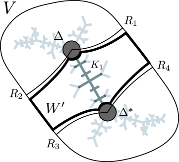
Figure 1: The heavy curves show the boundary of $W^{\prime}$.

Next we choose a sufficiently small round disk $\Delta^{\prime}\subset V_{1}$ about $\beta_{1}$ so that $g_{1}^{-1}(\Delta^{\prime})$ consists of two topological disks $\Delta$ and $\Delta^{\ast}$ with $\beta_{1}\in\Delta\Subset\Delta^{\prime}$ and $\beta_{1}^{\ast}\in\Delta^{\ast}$. We also choose a sufficiently small $\eta>0$ such that if $t$ satisfies $|\theta_{i}-t|<\eta$ for some $1\leq i\leq 4$, then $R_{g}(t)$ intersects with either $\Delta$ or $\Delta^{\ast}$.

Now $V=U_{g}(r)$ minus the union

$${\left(R_{g}(\theta_{1}-\eta)\cup R_{g}(\theta_{2}+\eta)\cup\overline{\Delta}\right)}\sqcup{\left(R_{g}(\theta_{3}-\eta)\cup R_{g}(\theta_{4}+\eta)\cup\overline{\Delta^{\ast}}\right)}$$

consists of three topological disks. We define $W^{\prime}$ by the one containing $K_{1}-\overline{\Delta}\cup\overline{\Delta^{\ast}}$.

Let $W_{1}$ denote the topological disk that is the connected component of $W^{\prime}\cap V_{1}$ containing the critical point of $g_{1}$. Since $W_{1}\subset V_{1}\Subset g^{-m}(V)$, the sets $W_{1}$, $g(W_{1})$, $\ldots$, $g^{m-1}(W_{1})$ are all defined and disjoint.

Now the inverse limit of the family ${\left\{g_{1}:g_{1}^{-n-1}(W_{1})\to g_{1}^{-n}(W_{1})\right\}}_{n\geq 0}$, denoted by $\underset{\longleftarrow}{\lim}(g_{1},W_{1})$, is a proper subset of $\mathcal{X}_{1}=\underset{\longleftarrow}{\lim}(g_{1},V_{1})$.

Set $\mathcal{Y}_{1}:=\underset{\longleftarrow}{\lim}(g_{1},W_{1})\subset\mathcal{X}_{1}$. Let us check that $\mathcal{Y}_{1}\approx\mathcal{X}_{1}$. By definition $V_{1}-W_{1}$ consists of disjoint topological disks and does not intersects $P(g_{1})$ since we take a sufficiently small $\Delta^{\prime}$. (Recall that $g$ is infinitely renormalizable, so the $\beta$-fixed point is at a certain distance away from the postcritical set $P(g)$. See [17, Theorem 8.1] for example. This is the only part we use the infinite renormalizability.) Thus $g_{1}:g_{1}^{-n-1}(V_{1})\to g_{1}^{-n}(V_{1})$ is isotopic to $g_{1}:g_{1}^{-n-1}(W_{1})\to g_{1}^{-n}(W_{1})$ for each $n\geq 0$ and this isotopy gives a homeomorphism between the inverse limits.

Let $\mathcal{Y}_{1}^{\ast}$ be the embedding of $\mathcal{Y}_{1}$ into $\mathcal{X}$ by the map $\iota$. For all $0\leq i<m$, the sets $\hat{g}^{i}(\mathcal{Y}_{1}^{\ast})$ are defined and disjoint since their projections $g^{i}(W_{1})$ are defined and disjoint. Hence we have (a) and (b) of the statement.

Proof of (c). Set $\mathcal{B}:=\mathcal{Y}-\bigsqcup_{i=0}^{m-1}\hat{g}^{i}(\overline{\mathcal{Y}_{1}^{\ast}})$. Now it is enough to show that $\mathcal{B}$ is homeomorphic to the block $\mathcal{B}_{s}$ associated with $f_{s}$, that is,

$$\mathcal{B}_{s}~{}=~{}\mathcal{N}_{s}-\overline{\hat{A}_{s}(r)}\cup\bigsqcup_{i=0}^{m-1}\hat{f}_{s}^{i}(\overline{\hat{D}_{s}(1/r)})~{}=~{}\pi_{s}^{-1}(U_{s}(r))-\bigsqcup_{i=0}^{m-1}\hat{f}_{s}^{i}(\overline{\hat{D}_{s}(1/r)}).$$

Here we take the same $r$ as in the construction of $V=U_{g}(r)$. For later use we also set $V_{s}:=U_{s}(r)$.

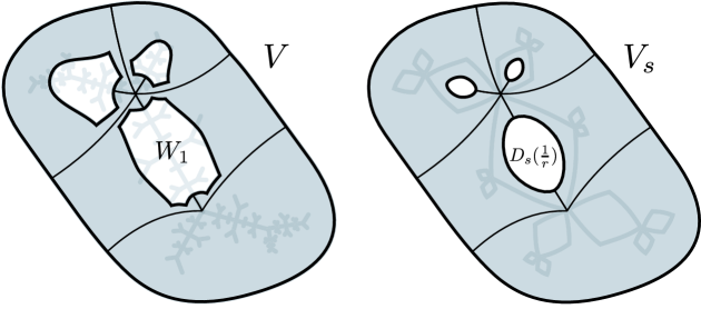
Figure 2: The shaded region show $B$ and $B_{s}$ with their markings drawn in.

We first work with the dynamics downstairs. Set $B:=V-\bigsqcup_{i=0}^{m-1}g^{i}(\overline{W_{1}})$ and mark $B$ with some arcs given as follows (See Figure 2, left): First join $g(\beta_{1})$ and $\partial g(W_{1})$ by an arc $\delta$ within $g(\Delta)$. Since $g:W_{1}\to g(W_{1})$ is a branched covering, the pull-back $g^{-1}(\delta)$ has two components in $\Delta$ and $\Delta^{\ast}$. Now the markings are given by $g^{-1}(\delta)$, $\delta$, $g(\delta),\ldots,g^{m-2}(\delta)$ and all of the forward images of the supporting rays $\bigcup_{j=1}^{4}R_{j}$. The markings decompose $B$ into finitely many pieces that are all topological disks. Note that the boundary of each piece intersects the equipotential $E_{g}(r)$ and at least two external rays.

Correspondingly, set $B_{s}:=V_{s}-\bigsqcup_{i=1}^{m-1}f_{s}^{i}(\overline{D_{s}(1/r)})$, and complete the marking of $B_{s}$ by taking all the forward images of supporting rays of $D_{s}$ and small arcs from each point in the cycle $O_{s}$ to the corresponding equipotentials $f_{s}^{i}(I_{s}(1/r))$ (Figure 2, right). The markings also decompose $B_{s}$ into some pieces as in the case of $B$.

Clearly, there is a homeomorphism $\phi$ from $B$ to $B_{s}$ respecting the configuration of the markings which in particular sends the supporting external rays into the supporting external rays without changing angles.

Lifting the homeomorphism. Now we claim: The map $\phi$ lifts to a homeomorphism $\hat{\phi}$ from $\pi^{-1}(B)$ in $\mathcal{Y}$ to $\pi_{s}^{-1}(B_{s})$ in the regular leaf space $\mathcal{R}_{s}$.

The proof requires the notion of external rays upstairs. Any backward sequence of external rays $R_{s}(\theta_{0})\leftarrow R_{s}(\theta_{-1})\leftarrow R_{s}(\theta_{-2})\leftarrow\cdots$ with $2\theta_{-n}=\theta_{-n+1}$ corresponds to an arc in $\mathcal{R}_{s}$. Each of such arcs is parameterized by “angles” of the form $\hat{\theta}=(\theta_{0},\theta_{-1},\ldots)$ and we denote it by $R_{s}(\hat{\theta})$. We define external rays $R_{g}(\hat{\theta})$ of $\mathcal{X}$ in the same way. (Note that such angles $\{\hat{\theta}\}$ and $\mathcal{S}^{1}=\underset{\longleftarrow}{\lim}(f_{0},\mathbb{S}^{1})$ has a one-to-one correspondence.)

Recall that by construction of $W_{1}$, the postcritical set $P(g)$ is contained in $\bigcup_{i=0}^{m-1}g^{i}(W_{1})$ so $g:g^{-n-1}(B)\to g^{-n}(B)$ is a covering map for each $n\geq 0$. Let $\Pi$ be one of the open pieces of $B$ decomposed by the markings. Since $\Pi$ is disjoint from the postcritical set, on each path-connected component $\hat{\Pi}$ of $\pi^{-1}(\Pi)$ (we call it a “plaque”) the projection $\pi|~{}\hat{\Pi}\to\Pi$ is a homeomorphism. Moreover, since $\partial\Pi$ intersects with two external rays, the plaque $\hat{\Pi}$ intersects with two external rays upstairs. Thus the angles of these rays upstairs determine the plaques of $\pi^{-1}(\Pi)$.

We have exactly the same situation for $B_{s}$. For $\Pi_{s}:=\phi(\Pi)$, which is one of the compact pieces of $B_{s}$ disjoint from $P(f_{s})$, we have a natural homeomorphic lift $\hat{\phi}:\pi^{-1}(\Pi)\to\pi_{s}^{-1}(\Pi_{s})$ which sends external rays upstairs on the boundary to those without changing the angles.

Now we have the desired homeomorphism $\hat{\phi}:\pi^{-1}(B)\to\pi_{s}^{-1}(B_{s})$ by gluing all of such $\hat{\phi}:\pi^{-1}(\Pi)\to\pi_{s}^{-1}(\Pi_{s})$ according to the angles of boundary external rays upstairs.

Extending the homeomorphism. We want to extend the homeomorphism $\hat{\phi}:\pi^{-1}(B)\to\pi_{s}^{-1}(B_{s})$ to $\hat{\phi}:\mathcal{B}\to\mathcal{B}_{s}$. To extend $\hat{\phi}$ to $\mathcal{B}-\pi^{-1}(B)$, we first describe what this remaining set is.

It may be easier to start with the dynamics of $f_{s}$. There are two types of backward orbits which start at the cyclic Fatou components $D_{s},f_{s}(D_{s}),\ldots,f_{s}^{m-1}(D_{s})$: One passes through $D_{s}$ infinitely many times, and one does only finitely many times. Correspondingly, there are two kinds of path-connected components of $\pi_{s}^{-1}(V_{s}-B_{s})$: One which is contained in the compact solenoidal cones $\bigsqcup_{i=0}^{m-1}\hat{f}_{s}^{i}(\overline{\hat{D}_{s}(1/r)})$, and one which is not. In particular, the latter is a closed disk in $\mathcal{B}_{s}$. Thus $\mathcal{B}_{s}-\pi_{s}^{-1}(B_{s})$ consists of such disks.

We have the same situation in the dynamics of $g$. Any path-connected component of $\pi^{-1}(V-B)$ is either contained in the closure of $\mathcal{Y}_{1}^{\ast}=\iota(\underset{\longleftarrow}{\lim}(g_{1},W_{1}))$; or not contained. The latter consists of orbits that escape from the nest of the renormalization so it is a closed disk in $\mathcal{B}$. Thus $\mathcal{B}-\pi^{-1}(B)$ also consists of closed disks.

Hence it is enough to extend $\hat{\phi}$ to such “escaping” orbits in $\mathcal{B}$. Let us choose a homeomorphic extension of $\phi$ which maps $V$ to $V_{s}$ and $g^{i}(W_{1})$ to $f_{s}^{i}(D_{s}(1/r))$ for all $0\leq i<m-1$. According to the markings on $\mathcal{B}$ and $\mathcal{B}_{s}$, the path-connected components of $\mathcal{B}-\pi^{-1}(B)$ and $\mathcal{B}_{s}-\pi_{s}^{-1}(B)$ are labeled by the angles of external rays. Thus there is a natural homeomorphic lift of the extended $\phi$ over those components. This gives a desired homeomorphism.

$\blacksquare$(Proposition 5)

Proof of Theorem 4 (The Structure Theorem). One can inductively apply the argument of Proposition 5 to each level of the renormalization ${\left\{g_{n}=f_{c}^{p_{n}}|~{}U_{n}\to V_{n}\right\}}_{n\geq 0}$, by setting $g:=g_{n}$ and $g_{1}:=g_{n+1}$.

We first apply the proposition with $n=0$. Then we construct $W_{1}$ and $\mathcal{B}=\mathcal{B}_{0}$ homeomorphic to $\mathcal{B}_{s_{0}}$. Next we apply the proposition with $n=1$. When we take modified $g_{1}:U_{1}\to V_{1}$ and $g_{2}:U_{2}\to V_{2}$ (i.e., when we replace $V_{1}$ by $V_{1}:=U_{g_{1}}(r_{1})$, etc.), we take a smaller $1<r_{2}<r_{g_{2}}$ so that $U_{2}:=U_{g_{2}}(\sqrt{r_{2}})$ and $V_{2}:=U_{g_{2}}(r_{2})$ satisfy the original condition

$$U_{2}~{}\Subset~{}V_{2}~{}\Subset~{}g_{1}^{-m_{1}}(V_{1})~{}\Subset~{}U_{1}~{}\Subset~{}V_{1}$$

and the extra condition

$$V_{2}\sqcup g_{1}(V_{2})\sqcup\cdots\sqcup g_{1}^{m_{1}-1}(V_{2})~{}\Subset~{}W_{1}.$$

As we construct $W_{1}\subset V_{1}$, we construct $W_{2}\subset V_{2}$ so that $\mathcal{Y}_{2}:=\underset{\longleftarrow}{\lim}(g_{2},W_{2})$ is homeomorphic to $\mathcal{X}_{2}=\underset{\longleftarrow}{\lim}(g_{2},V_{1})$ and that $\mathcal{Y}_{2}^{\ast},~{}\hat{g}_{1}(\mathcal{Y}_{2}^{\ast}),\ldots,\hat{g}_{1}^{m_{1}-1}(\mathcal{Y}_{2}^{\ast})$ are defined and disjoint, where $\mathcal{Y}_{2}^{\ast}$ denote the natural embedding of $\mathcal{Y}_{2}$ into $\mathcal{X}_{1}=\underset{\longleftarrow}{\lim}(g_{1},V_{1})$. By the extra condition above, we have

$$\mathcal{Y}_{2}^{\ast}\sqcup\hat{g}_{1}(\mathcal{Y}_{2}^{\ast})\sqcup\cdots\sqcup\hat{g}_{1}^{m_{1}-1}(\mathcal{Y}_{2}^{\ast})~{}\Subset~{}\mathcal{Y}_{1}.$$

Moreover, we have a block $\mathcal{B}_{1}^{\prime}~{}:=~{}\mathcal{Y}_{1}-\bigsqcup_{i=0}^{m_{1}-1}\hat{g}_{1}^{i}(\overline{\mathcal{Y}_{2}^{\ast}})$ homeomorphic to $\mathcal{B}_{s_{1}}$. Finally we define $\mathcal{B}_{1}$ by the natural embedding of $\mathcal{B}_{1}^{\prime}$ into $\mathcal{X}_{0}=\underset{\longleftarrow}{\lim}(g_{0},V_{0})\subset\mathcal{N}_{c}$.

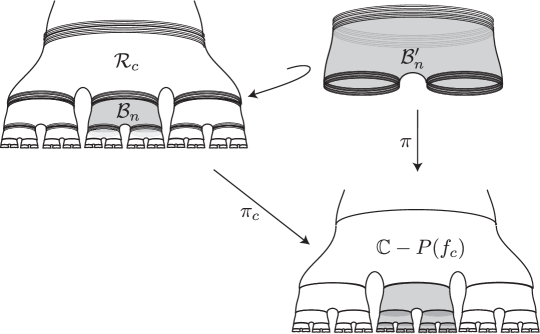
Figure 3: A caricature of the tree structure of $\mathcal{R}_{c}$. It comes from a natural tree structure in the set $\mathbb{C}-P(f_{c})$.

Clearly the same argument works for the other levels $n\geq 2$. Note that $\mathcal{B}_{n}^{\prime}$ constructed as above is contained in $\underset{\longleftarrow}{\lim}(g_{n},W_{n})$. (See Figure 3.) So we need to iterate the natural embeddings

$$\mathcal{B}_{n}^{\prime}~{}\hookrightarrow~{}\underset{\longleftarrow}{\lim}(g_{n-1},W_{n-1})~{}\hookrightarrow~{}\cdots\hookrightarrow~{}\underset{\longleftarrow}{\lim}(g_{1},W_{1})~{}\hookrightarrow~{}\underset{\longleftarrow}{\lim}(g_{0},V_{0})$$

to obtain $\mathcal{B}_{n}\subset\mathcal{N}_{c}$.

In addition, we replace $\mathcal{B}_{0}$ by the set $\mathcal{B}_{0}\cup\overline{\hat{A}(r_{0})}-{\left\{\hat{\infty}\right\}}$ (where $\hat{A}(r_{0})$ is a solenoidal cone, with $r_{0}$ satisfying $V_{0}=U_{g_{0}}(r_{0})$) so that $\mathcal{B}_{0}$ covers the neighborhood of $\hat{\infty}$. Then we have property 1 of the statement. Properties 2, 3, and 4 of the statement are clear by the construction of blocks.

Now every backward orbit that leaves $P(f_{c})\cup{\left\{\infty\right\}}$ is contained in one of such blocks $\{\hat{f}_{c}^{i}(\mathcal{B}_{n})\}_{n,i}$. Since $f_{c}$ is persistently recurrent, the set $\widehat{P(f_{c})}\cup{\left\{\hat{\infty}\right\}}$ consists of all irregular points so the union of the blocks $\{\hat{f}_{c}^{i}(\mathcal{B}_{n})\}_{n,i}$ coincide with $\mathcal{R}_{c}$. Thus we have 4 and 5 of the statement.

$\blacksquare$

3.2 Buildings at finite level

To end this section we show a proposition that is important for the arguments in the next section.

For an infinite sequence of combinatorics ${\left\{s_{0},s_{1},\ldots\right\}}$, its subsequence ${\left\{s_{0},s_{1},\ldots,s_{n}\right\}}$ determines a superattracting parameter $\sigma_{n}$. More precisely, for $\beta$-fixed point $\beta(g_{n+1})$ of $g_{n+1}=f_{c}^{p_{n+1}}$, its forward orbit $O_{n+1}$ by $f_{c}$ forms a repelling periodic point. Then its ray portrait $\mathrm{rp}(O_{n+1})$ determines a superattracting quadratic map $f_{\sigma_{n}}$. It is known that it depends only on the sub-combinatorics ${\left\{s_{0},s_{1},\ldots,s_{n}\right\}}$ of the renormalizations.

For persistently recurrent infinitely renormalizable $f_{c}$ as above, we define

$$\mathcal{Q}_{n}~{}:=~{}\mathcal{R}_{c}-\bigsqcup_{k=n+1}^{\infty}\bigsqcup_{i=0}^{p_{k}-1}\hat{f}_{c}^{i}(\mathcal{B}_{k}).$$

Then we have:

Proposition 6.

For $f_{c}$ as above, let $\mathcal{Q}_{n}$ be the set defined as above. Then we have a homeomorphism $h_{n}$ between $\mathcal{Q}_{n}$ and $\mathcal{Q}_{\sigma_{n}}$.

Proof. The proof is almost straightforward by Proposition 5. In fact, we can apply the same argument by setting $g:=g_{0}$ and $g_{1}:=g_{n+1}$. $\blacksquare$

4 Rigidity

In this section we prove the Main Theorem of the paper which is the following:

Theorem 7 (Main Theorem).

Let $c$ be a non-real complex number, such that the map $f_{c}$ is infinitely renormalizable with a-priori bounds. If $h:\mathcal{R}_{c}\rightarrow\mathcal{R}_{c^{\prime}}$ is oriented homeomorphism, then $c$ and $c^{\prime}$ belong to the same combinatorial class.

From the point of view of the parameter plane, it is known that $c$ is combinatorially rigid if and only if the Mandelbrot set is locally connected at $c$. In view of that, our main theorem has the following corollary.

Corollary 8.

Assume that $c$ is as in the Main Theorem and that the Mandelbrot set is locally connected (MLC) at $c$, then $c=c^{\prime}$.

In [15], Lyubich proved MLC for $f_{c}$ with a-priori bounds with some extra condition on combinatorics, called secondary limb condition. In this direction, there is recent work by Jeremy Kahn [6] and Kahn and Lyubich [7] where they prove a-priori bounds and MLC for infinite renormalizable parameters with special combinatorics.

4.1 Combinatorics of quadratic polynomials

There are several models describing the combinatorics of quadratic polynomials, a comprehensive text can be found in [1], in this paper we are going to adopt the description given by rational laminations. Any quadratic polynomial $f_{c}$ with $c$ in the Mandelbrot set, determines a relation, called the rational lamination of $f_{c}$, in $\mathbb{Q}/\mathbb{Z}$. Given $\theta$ and $\theta^{\prime}$ in $\mathbb{Q}/\mathbb{Z}$, we say that $\theta\sim\theta^{\prime}$ if the external rays $R_{\theta}$ and $R_{\theta^{\prime}}$ land at the same point in the Julia set $J(f_{c})$. Jan Kiwi gave a set of properties which guarantee that if a given relation in $\mathbb{Q}/\mathbb{Z}$ satisfies these properties then the relation is a rational lamination of some polynomial $P$, the interested reader can consult [11]. For us, the most relevant property of rational laminations is the following:

Lemma 9.

Let $R$ and $R^{\prime}$ be two rational laminations, assume that there is $\theta\in\mathbb{Q}/\mathbb{Z}$ such that each class in $R^{\prime}$ is obtained by rotating a class in $R$ by angle $\theta$. Then $\theta=0\,\mod(1)$.

Let us call a leaf $L$ in $\mathcal{R}_{c}$ repelling if it contains a repelling periodic point of $\hat{f}_{c}$. Clearly, every repelling leaf is invariant under some iterate of $\hat{f}_{c}$, the converse is not true in general, because in the presence of parabolic point there are invariant leaves without periodic points. In the case of the dyadic solenoid $\mathcal{S}^{1}$ if a leaf $L\subset\mathcal{S}^{1}$ is invariant under some iterate of $\hat{f}_{0}$, then $L$ is repelling. The fact that all periodic leaves in $\mathcal{S}^{1}$ are repelling allow us to lift combinatorial properties of periodic points in $J(f_{c})$ to repelling leaves in $\mathcal{R}_{c}$.

More precisely, let $L$ be a repelling leaf in $\mathcal{R}_{c}$ and let $\mathcal{S}_{r}$ some solenoidal equipotential, the intersection $L\cap\mathcal{S}_{r}$ consists of some leaves in $\mathcal{S}_{r}$ under the canonical identification, it turns out, every such leaf is repelling in $\mathcal{S}^{1}$ under $\hat{f}_{0}$. Moreover, the pullback to $L$ of each of these periodic points is precisely the intersection of a periodic solenoidal external ray landing at the periodic point of $L$.

In the dynamical plane, if $p$ is a periodic point in the Julia set $J(f_{c})$ then $p$ is the landing point of external rays which are periodic under $f_{c}$, see [19], if the periodic lift $\hat{p}$ belongs to the regular part, then there are periodic solenoidal external rays landing at $\hat{p}$ in $L(\hat{p})$, each of these solenoidal external rays will intersect a leaf of a solenoidal equipotential. As a consequence we have:

Lemma 10.

Two leaves $\mathcal{S}_{r}$, coming from periodic leaves in $\mathcal{S}^{1}$, belong to the same leaf $L$ in $\mathcal{R}_{c}$ if and only if they intersect periodic solenoidal external rays landing in the same point in $\pi^{-1}(J(f_{c}))\cup\mathcal{R}_{c}$.

We will see that, for quadratic polynomials with a-priori bounds, repelling leaves have topological relevance. Such was the approach in [3] (see also [2]) to prove rigidity for hyperbolic maps and complex semi-hyperbolic. We can resume the main results in [3] with the following theorem:

Theorem 11.

Let $h:\mathcal{N}_{c}\rightarrow\mathcal{N}_{c^{\prime}}$ be a homeomorphism between natural extensions, such that:

1. $h(\hat{\infty})=\hat{\infty}$; and

2. $h$ sends repelling leaves into repelling leaves.

Then $f_{c}$ and $f_{c^{\prime}}$ belong to the same combinatorial class.

The proof of this theorem is decomposed in three statements; Lemma 12 whose proof can be found in [3], Proposition 13 due to Jaroslaw Kwapisz [12], and Lemma 14. The first starts by noting that the foliation of the solenoidal cone by solenoidal equipotentials defines a local base of neighborhoods at $\hat{\infty}$ in $\mathcal{N}_{c}$. Hence, given a homeomorphism $h$ as in Theorem 11, we can find a solenoidal equipotential $\mathcal{S}_{r}$ whose image lies between two solenoidal equipotentials. Recall that a solenoidal equipotential $\mathcal{S}_{r}$ has associated a canonical homeomorphism $\phi_{R}:\mathcal{S}_{r}\rightarrow\mathcal{S}^{1}$, moreover, $\phi_{R^{2}}\circ\hat{f}_{c}\circ\phi_{R}^{-1}=\hat{f}_{0}$. Hence, we are in the following situation:

Lemma 12.

Let $e:\mathcal{S}^{1}\rightarrow\mathcal{S}^{1}\times(0,1)$ be a topological embedding, then there is a map $e^{\prime}$ isotopic to $e$ such that $e^{\prime}(\mathcal{S}^{1})=\mathcal{S}^{1}\times{1/2}$.

We can pull back the isotopy in this lemma, to an isotopy defined on $\mathcal{S}_{r}$ which extends to an isotopy defined on a neighborhood of $\mathcal{S}_{r}$. Hence, we can find a homeomorphism $h^{\prime}$, isotopic to $h$, that sends homeomorphically a solenoidal equipotential into a solenoidal equipotential. With the canonical homeomorphism of solenoidal equipotentials to $\mathcal{S}^{1}$, $h^{\prime}$ induces a self homeomorphism of the dyadic solenoid $\mathcal{S}^{1}$. Now, as described by Kwapisz in [12], each homotopic class of homeomorphisms of $\mathcal{S}^{1}$ is uniquely represented by a map with a special form:

Proposition 13 (Kwapisz).

Let $\phi:\mathcal{S}^{1}\rightarrow\mathcal{S}^{1}$ be a homeomorphism of the dyadic solenoid, then there exist $n$ and an element $\tau\in\mathcal{S}^{1}$ such that $\phi$ is isotopic to $\hat{z}\mapsto\tau\hat{f}^{n}_{0}(\hat{z})$.

The number $n$ is uniquely determined by the homotopic class of $h^{\prime}$, so if we post-compose $h^{\prime}$ with $f^{-n}_{c^{\prime}}$, Proposition 13 implies that we can find a new homeomorphism from $\mathcal{N}_{c}$ to $\mathcal{N}_{c^{\prime}}$ sending one solenoidal equipotential into a solenoidal equipotential, such that under the canonical identification, the map between these solenoidal equipotentials is just the left translation by $\tau$ of the dyadic solenoid $\mathcal{S}^{1}$.

All isotopies above, and the map $\hat{f}_{c^{\prime}}$, send repelling leaves into repelling leaves, so our new homeomorphism will also send repelling leaves into repelling leaves. By the previous lemmas, if $h$ is a homeomorphism like in Theorem 11, then we can assume that $h$ sends a solenoidal equipotential $\mathcal{S}_{r}$ homeomorphically into a solenoidal equipotential and, that under canonical isomorphisms, the map $h$ restricted to $\mathcal{S}_{r}$ is just a translation $\tau$ by an element in $\mathcal{S}^{1}$. Now the combinatorial information of $f_{c}$ give us more restrictions on the isotopy class of $h$:

Lemma 14.

Assume $h$ is a homeomorphism like in Theorem 11, then the induced translation $\tau$ in Proposition 13 is homotopic to the identity.

Proof. Let us consider the restriction of $h$ to the solenoidal equipotential $\mathcal{S}_{r}$ such that $h(\mathcal{S}_{r})$ is also a solenoidal equipotential, under canonical homeomorphisms the map $H=h|\mathcal{S}_{r}$ is a map from $\mathcal{S}^{1}$ into itself. We assume that $H$ has the form $\hat{z}\mapsto\tau\hat{z}$. By Lemma 10, $h|\mathcal{S}_{r}$ sends repelling leaves into repelling leaves.

Let $L$ be a periodic leaf in $\mathcal{S}^{1}$ with $\hat{\theta}$ the periodic point in $L$, let $\hat{\theta}^{\prime}$ be the periodic point in $H(L)$. By sliding $\mathcal{S}^{1}$ along $h|\mathcal{S}_{r}(L)$ to send $H(\hat{\theta})$ to $\hat{\theta}^{\prime}$, this operation induces a new map $H^{\prime}$ in the isotopy class of $H$, which satisfies $H(\hat{\theta})=\tau^{\prime}\hat{\theta}=\hat{\theta}$, since $\hat{\theta}$ and $\hat{\theta}^{\prime}$ are periodic in $\mathcal{S}^{1}$, $\tau^{\prime}$ must be periodic as well. Hence, the map $H^{\prime}$ leaves the set of periodic points in $\mathcal{S}^{1}$ invariant.

Now, periodic points in $\mathcal{S}^{1}$ are determined by the first coordinate. The translation $\tau$ induces a rotation in the set of periodic angles which extends to a rotation on the rational lamination. By Lemma 9 this implies that the rational laminations are the same, and that the translation $\tau^{\prime}$ is the identity, by construction $\tau^{\prime}$ is isotopic to $\tau$. $\blacksquare$

Proof. [Proof of Theorem 11] As a consequence of the previous Lemma the rational laminations of $f_{c}$ and $f_{c^{\prime}}$ are the same. This implies that $c$ and $c^{\prime}$ belong to the same combinatorial class. $\blacksquare$

4.2 Ends of the regular part

A path $\gamma:[0,\infty)\rightarrow\mathcal{R}_{c}$ is said to escape to infinity if it leaves every compact set $K\subset\mathcal{R}_{c}$. we define an end of $\mathcal{R}_{c}$ to be an equivalence class of paths escaping to infinity. Let $\gamma$ and $\sigma$ two paths escaping to infinity, we say that $\gamma$ and $\sigma$ access the same end if for every compact set $K\subset\mathcal{R}_{c}$, the paths $\gamma$ and $\sigma$ eventually belong to the same connected component of $\mathcal{R}_{c}\setminus K$. Consider the set $End(\mathcal{R}_{c})$ consisting of $\mathcal{R}_{c}$ union with the abstract set of ends.

Let $f_{c}$ be an infinitely renormalizable quadratic polynomial with a-priori bounds, by Theorem 2 the regular part $\mathcal{R}_{c}$ is locally compact and then $End(\mathcal{R}_{c})$ is a compact set, which we will call the end compactification of $\mathcal{R}_{c}$.

Proposition 15.

Let $f_{c}$ be an infinite renormalizable quadratic polynomial with a-priori bounds, then $End(\mathcal{R}_{c})$ is homeomorphic to $\mathcal{N}_{c}$.

Proof. We will show that there exist a bijection $\Phi$ between the set of irregular points and the set of ends. Let $\hat{i}$ be an irregular point in $\mathcal{N}_{c}$, let $i_{0}=\pi(\hat{i})$ and take any $z_{0}\in\mathbb{C}\setminus\omega(c)$. Since $\omega(c)$ is a Cantor set, there is a path $\sigma$ be a path connecting $z_{0}$ with $i_{0}$ which intersects $\omega(c)$ only at $i_{0}$. We can lift the path $\sigma$ to $\mathcal{N}_{c}$ to a path $\hat{\sigma}$ from a point in the fiber of $z_{0}$ connecting to $\hat{i}$. By construction, the path $\hat{\sigma}$ intersects $\mathcal{I}_{c}$ at $\hat{i}$, then the restriction of $\hat{\sigma}$ to $\mathcal{R}_{c}$ is a path escaping to infinity. Let $\Phi(\hat{i})=[\hat{\sigma}]$, where $[\hat{\sigma}]$ is the end represented by $\hat{\sigma}$. Now we check that $\Phi$ is well defined, let $\hat{\sigma}$ and $\hat{\sigma^{\prime}}$ be two paths in $\mathcal{N}_{c}$ intersecting the irregular set only at the end point $\hat{i}$. These paths do not need to start at the same point or belong to the same leaf. Let $L$ be the leaf containing $\sigma([0,1))$ in $\mathcal{R}_{c}$. Since every leaf is dense in $\mathcal{R}_{c}$ and is simply connected, we can construct a family of paths $\hat{\sigma_{n}}$ in $L$, ending at $\hat{i}$ and such that $\hat{\sigma}_{n}\rightarrow\hat{\sigma}^{\prime}$ pointwise. Let $K$ be any compact set in $\mathcal{R}_{c}$, and $U$ be a connected component of $\mathcal{R}_{c}\setminus K$ which eventually contains $\hat{\sigma}^{\prime}$. Since $U$ is open, there is a $N$ such that $\hat{\sigma}_{N}$ also eventually belongs to $U$, but $\hat{\sigma}$ and $\hat{\sigma}_{N}$ belong to the same path connected component (same leaf), thus $\hat{\sigma}$ must also be eventually contained in $U$.

To see that $\Phi$ is injective, let $\hat{i}$ and $\hat{i}^{\prime}$ be two irregular points, since the projection $\pi$ is a homeomorphism between the set of irregular points and $\omega(c)$ we have $\pi(\hat{i})\neq\pi(\hat{i}^{\prime})$, and any two paths $\phi$ and $\phi^{\prime}$ escaping to $\hat{i}$ and $\hat{i}^{\prime}$ respectively, must eventually belong to different components of some level of renormalization.

Finally, let us prove that $\Phi$ is surjective. Let $e$ be an end of $\mathcal{R}_{c}$, and consider $\phi$ a path escaping to $e$. Let $D_{r}$ be a closed ball containing $J(f)$. For each level of renormalization $n$, let $Q_{n}$ be a family of disjoint open neighborhoods of the little Julia sets of level $n$, if these Julia set touch, we can shrink the domains a little to make them disjoints as in the proof of Theorem 4. Let $W_{n}$ be the union of the domains in $Q_{n}$. Then $K_{n}=B_{r}\setminus Q_{n}$ is a compact set in $\mathbb{C}\setminus\omega_{c}$. Thus $\pi^{-1}(K_{n})$ is compact in $\mathcal{R}_{c}$, by definition the path $\phi$ must eventually escape $\pi^{-1}(K_{n})$. It follows that the projection $\pi(\phi)$ eventually belongs either to a neighborhood of infinity, and then $\phi$ escapes to $\hat{\infty}$, or to a domain in $Q_{n}$, say $V_{n}$, by the disjoint property of the sets in $Q_{n}$, it is clear that $V_{n+1}$ is contained in $V_{n}$. By construction, the domains $\{V_{n}\}$ shrink to a point $i_{0}$ in $\omega(c)$. This process can be repeated for every coordinate of $\phi$ to get a sequence of points $\{i_{n}\}$ in $\omega(c)$ which are the coordinates of a point $\hat{i}$ in $\widehat{\omega(c)}$. Since $f$ is persistently recurrent $\hat{i}$ is irregular. $\blacksquare$

On the remaining part of the paper $h$ will denote a homeomorphism of the regular parts of two infinite renormalizable quadratic polynomials $f_{c}$ and $f_{c^{\prime}}$ with a-priori bounds.

Corollary 16.

The map $h$ admits an extension to a homeomorphism $\tilde{h}:\mathcal{N}_{c}\rightarrow\mathcal{N}_{c^{\prime}}$ of the regular extensions. Moreover, $\tilde{h}(\hat{\infty})=\hat{\infty}$.

Proof. By Proposition 15 the map $h$ extends to the natural extensions sending irregular points to irregular points, and by Lemma 3 the point $\hat{\infty}$ is the only isolated irregular point, hence $h(\hat{\infty})=\hat{\infty}$. $\blacksquare$

4.3 Topology of Periodic leaves

Since leaves are path connected components of $\mathcal{R}_{c}$, given a leaf $L\subset\mathcal{R}_{c}$ we can consider how many access to $\hat{\infty}$ the leave has. That is, the number of path components of $L\setminus K$ that are connected to $\hat{\infty}$ in $\mathcal{N}_{c}$, for a suitable large compact set $K\subset\mathcal{R}_{c}$. Note that a leaf has access to points in $\omega(c)$ if and only if intersects infinitely many levels in the tree structure of $\mathcal{R}_{c}$. However, this is not the case for repelling leaves:

Lemma 17.

Let $L$ be a repelling leaf, then $L$ there is a level $n$ such that $L\subset\mathcal{Q}_{n}$. In this case, $L$ has access only to $\hat{\infty}$.

Proof. Let $\hat{p}$ be the periodic point in $L$ and let $p=\pi(p)$. Since $f_{c}$ is infinite renormalizable, $p$ is repelling, and therefore it must belong to the Julia set $J(f_{c})$, moreover, the inverse of the classical Königs linearization coordinate around $p$ provides a global uniformization coordinate for $L$. From this uniformization it follows that a point $\hat{z}$ in $\mathcal{R}_{c}$ belongs to $L$ only if the coordinates of $\hat{z}$ converge to the cycle of $p$.

Since the intersection of the renormalization domains is just the postcritical set, we can find a level $n+1$ of the renormalization such that the orbit of the renormalization domains of level $n+1$ is outside a neighborhood of the cycle of $p$. By this choice, no point in $L$ can intersect the level $n+1$ of the tree structure of $\mathcal{R}_{c}$. The statement of the lemma now follows. $\blacksquare$

When $f_{c}$ is superattracting, every leaf $L$ invariant under some iterate of $\hat{f}$ must contains a repelling periodic point and hence $L$ is repelling. In this case, there are no critical points in the Julia set $J(f_{c})$ so the fiber $\pi^{-1}(J(f_{c}))$ is compact. If $p$ is a periodic point in $J(f_{c})$. Let $\hat{p}$ be invariant lift of $p$ in $\mathcal{R}_{c}$, and $L(\hat{p})$ the leaf containing $\hat{p}$. From [3], we have the following:

Proposition 18.

The number of access of $L$ to $\hat{\infty}$ is equal to the number of external rays landing at $p$. Moreover, if $L$ is a leaf which has at least three access to infinity, then $L$ must be repelling.

Let us remark that in the superattracting case, Proposition 15 also holds, however, repelling leaves may have access to other irregular points. Nevertheless, if some repelling leaf $L$ has at least three access to $\hat{\infty}$ then by Proposition 18, the corresponding periodic point $p$ has at least three external rays landing at $p$. This situation only can happen if the imaginary part of $c$ is not 0.

Let us now go back to the case were $f_{c}$ is infinite renormalizable with a-priori bounds:

Lemma 19.

Let $f_{c}$ be infinite renormalizable with a-priori bounds, and let $L\subset\mathcal{R}_{c}$ be a leaf which has at access only to $\hat{\infty}$, and such that the number of access to infinity is at least 3, then $L$ must be a repelling leaf. Moreover, this implies that $Im(c)\neq 0$.

Proof. Since the only access to infinity of $L$ is $\hat{\infty}$, there is a level $n$ such that $L\subset\mathcal{Q}_{n}$. By Corollary 16 the map $h$ extends to the natural extensions and $\hat{\infty}$, so the image $h(L)$ is also a leave with the same number of access to $\hat{\infty}$. Regarding $L$ as a subset of $\mathcal{Q}_{n}$, the leaf $L$ has at least 3 access to $\infty$ in $\mathcal{Q}_{n}$ by Proposition 18 the leaf $L$ must be repelling in $\mathcal{Q}_{n}$ under dynamics of $\hat{f}_{s_{n}}$, by the block homeomorphism in the proof of Theorem 6, this implies that $L$ itself must be repelling under dynamics of $\hat{f}_{c}$. $\blacksquare$

Now we are ready to prove the Main Theorem:

Proof of Main Theorem. By Corollary 16, the map extends to a homemorphisms of natural extensions $\tilde{h}$ with $\tilde{h}(\hat{\infty})$. Since $Im(c)\neq 0$ then there exist a repelling leaf $L$ in $\mathcal{N}_{c}$ such that $L$ has at least three access to $\hat{\infty}$. This is a topological property, so $h(L)$ is also a leaf with at least 3 access to $\hat{\infty}$. By Lemma 19 $h(L)$ is also repelling and moreover $Im(c^{\prime})\neq 0$. In this way, $\tilde{h}$ sends a repelling leaf into a repelling leaf. By an isotopy argument similar to the one used in the proof of Lemma 14, we can see that this implies that $h$ sends repelling leaves into repelling leaves. Hence, $\tilde{h}$ satisfies the conditions of Theorem 11, which implies that $f_{c}$ and $f_{c^{\prime}}$ belong to the same combinatorial class. $\blacksquare$

	Carlos Cabrera
	Institute of Mathematics of the
	Polish Academy of Sciences
	ul. Śniadeckich 8
	00-956 Warszawa, Poland

	Tomoki Kawahira
	Graduate School of Mathematics
	Nagoya University
	Nagoya 464-8602, Japan

References

- [1] H. Bruin and D. Schleicher, Symbolic dynamics of quadratic polynomials, Mittag-Leffler Preprint Series (2002).
- [2] C. Cabrera, Towards classification of laminations associated to quadratic polynomials, Ph.d thesis, Stony Brook, 2005, http://www.math.sunysb.edu/cgi-bin/thesis.pl?thesis05-3.
- [3] , On the classification of laminations associated to quadratic polynomials, arXiv:math/0703159 (2006).
- [4] A. Douady and J. H. Hubbard, Étude dynamique des polynômes complexes I & II, Publ. Math. Orsay (1984).
- [5] John H. Hubbard and Ralph W. Oberste-Vorth, Hénon mappings in the complex domain. II. Projective and inductive limits of polynomials, Real and complex dynamical systems (Hillerød, 1993), NATO Adv. Sci. Inst. Ser. C Math. Phys. Sci., vol. 464, Kluwer Acad. Publ., Dordrecht, 1995, pp. 89–132.
- [6] J. Kahn, A priori bounds for some infinitely renormalizable quadratics. I. Bounded primitive combinatorics., arXiv:math.DS/0609045 (2006).
- [7] J. Kahn and M. Lyubich, A priori bounds for some infinitely renormalizable quadratics. II. Decorations., arXiv:math.DS/0609046 (2006).
- [8] V. Kaimanovich and M. Lyubich, Conformal and harmonic measures on laminations associated with rational maps, Mem. Amer. Math. Soc. 173 (2005), no. 820.
- [9] T. Kawahira, On the regular leaf space of the cauliflower, Kodai Math. J. (2003), no. 26, 167–178.
- [10] , Tessellation and Lyubich-Minsky laminations associated with quadratic maps I & II, arXiv:math.DS/0609280 & arXiv:math.DS/0609836 (2006).
- [11] J. Kiwi, Rational laminations of complex polynomials, Laminations and foliations in dynamics, geometry and topology (Stony Brook, NY, 1998), Contemp. Math., vol. 269, Amer. Math. Soc., Providence, RI, 2001, pp. 111–154.
- [12] J. Kwapisz, Homotopy and dynamics for homeomorphisms of solenoids and Knaster continua, Fund. Math. 168 (2001), no. 3, 251–278.
- [13] M. Lyubich, Dynamics of the rational transforms; the topological picture, Russian Math. Surveys (1986).
- [14] , Combinatorics, geometry and attractors of quasi-quadratic maps, Ann. of Math. (2) 140 (1994), no. 2, 347–404.
- [15] , Dynamics of quadratic polynomials. I, II, Acta Math. 178 (1997), no. 2, 185–247, 247–297.
- [16] M. Lyubich and Y. Minsky, Laminations in holomorphic dynamics, J. Diff. Geom. 47 (1997), 17 – 94.
- [17] C. McMullen, Complex dynamics and renormalization, Annals of Mathematics Studies, vol. 135, Princeton University Press, Princeton, NJ, 1994.
- [18] J. Milnor, Local connectivity of Julia sets: expository lectures, The Mandelbrot set, theme and variations, London Math. Soc. Lecture Note Ser., vol. 274, Cambridge Univ. Press, Cambridge, 2000, pp. 67–116.
- [19] , Periodic orbits, external rays and the Mandelbrot set: An expository account, Asterisque 261 (2000).
- [20] D. Sullivan, Bounds, quadratic differentials, and renormalization conjectures, A.M.S. centennial publications, Vol. II (Providence, RI, 1988), A.M.S., Providence, RI, 1992, pp. 417–466.