Dynamical Systems On Three Manifolds
Part II: 3-Manifolds, Heegaard Splittings and Three-Dimensional Systems

Abstract

The global behaviour of nonlinear systems is extremely important in control and systems theory since the usual local theories will only give information about a system in some neighbourhood of an operating point. Away from that point, the system may have totally different behaviour and so the theory developed for the local system will be useless for the global one.

In this paper we shall consider the analytical and topological structure of systems on 2- and 3- manifolds and show that it is possible to obtain systems with ’arbitrarily strange’ behaviour, i.e., arbitrary numbers of chaotic regimes which are knotted and linked in arbitrary ways. We shall do this by considering Heegaard Splittings of these manifolds and the resulting systems defined on the boundaries.
Keywords: Heegaard Splitting, Automorphic functions, Connected Sum, Fuchsian group, C-homeomorphisms.

1 Introduction

In a recent paper ([Banks & Song, 2006]), we have shown how to define general (analytic) systems on 2-manifolds by using the theory of automorphic functions. The importance of this theory to dynamical systems is that, globally, they are defined not on ‘flat’ Euclidean spaces, but on manifolds. In fact, it was shown in ([Banks & Song, 2006]) that the simple pendulum ‘sits’ naturally on a Klein bottle. In this paper, we consider the case of three-dimensional systems and derive some results on the nature of three-dimensional dynamical systems and the 3-manifolds on which they ‘live’.

The main difficulty compared with the 2-manifold case is that 3-manifold topology is much more complex. Indeed, there is no procedure for finding a complete set of topological invariants for a three manifold although a great many invariants have been found, surprisingly from quantum group theory ([Ohtsuki, 2001]). There we shall extend our 2-manifold theory coupled with Heegaard Splittings and Connected Sums to approach a theory of 3-dimensional dynamical systems.

2 Three Manifolds and Heegaard Splittings

We shall consider, in this paper, dynamical systems defined on 3-manifolds. A 3-manifold M is a separable metric space such that each point $x\in\emph{M}$ has an open neighbourhood, which is homeomorphic to $\mathbb{R}^{3}$ or $\mathbb{R}_{+}^{3}=\{x\in{\mathbb{R}^{3}}:\;x_{3}\geq{0}\}$, we can assume all the 3-manifolds we consider here are differentiable (or p.l.) manifolds since any 3-manifold has a unique p.l. or differentiable structure (see [Hempel, 1976]). Points in M which look locally like $\mathbb{R}^{3}$ are called boundary points. The set of all boundary points is denoted by $\partial\emph{M}$. Note that $\partial\partial\emph{M}=\emptyset$. A manifold which is compact and for which $\partial\emph{M}=\emptyset$ is called closed.

Definition 2.1

A Heegaard Splitting of a closed connected 3-manifold M is a pair $(C_{1},C_{2})$ of cubes with handles such that

$$M=C_{1}\cup C_{2}$$

and

$$C_{1}\cap C_{2}=\partial C_{1}=\partial C_{2}.$$

The following results are well known (see, e.g. [Hempel, 1976]):

Theorem 2.1

Every closed, connected 3-manifold has a Heegaard Splitting.

Proposition 2.1

There is exactly one nonorientable 3-manifold with a genus one Heegaard Splitting, the nonorientable 2-sphere bundle over $S^{1}$, i.e., the trivial gluing of two solid Klein bottle.

Let $(C_{1},C_{2})$ be a Heegaard Splitting of a 3-manifold M. A Heegaard diagram, $(C_{1};\partial D_{1},\cdots,\partial D_{n})$, for the splitting $(C_{1},C_{2})$ consists of a set $\{D_{1},\cdots,D_{n}\}$ of pairwise disjoint, properly embedded, 2-cells in $C_{2}$ which cut it into a 3-cell. We can regard M as being obtained from $C_{1}$ and $C_{2}$ by choosing a homeomorphism of $\partial C_{1}$ onto $\partial C_{2}$ which maps a standard set of longitudinal or meridian curves on $\partial C_{1}$ to $\{\partial D_{1},\cdots,\partial D_{n}\}$ situated on $\partial C_{2}$ (and extending this homeomorphism throughout $C_{1}$ and $C_{2}$). Lickorish ([Lickorish, 1962]) shows that such a surface homeomorphism can be generated (up to isotopy) by a sequence of C-homeomorphisms, i.e., homeomorphisms of the following form:

Take a nontrivial cycle l on the surface S, cut along l, twist one side of the cycle through $2\pi$ and reconnect the ‘two sides’ of l.

As an example, Fig 1 shows us how to get a trefoil knot from a trivial one in this way.

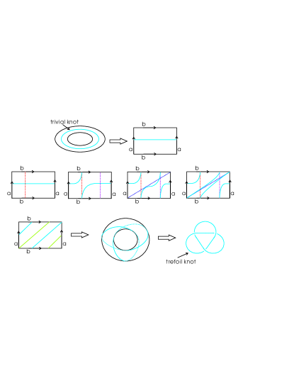
Figure 1: Generating a trefoil knot from a trivial one via C-homeomorphisms

We shall use this result to perform surgery on our 2-dimensional automorphic systems and their extensions to obtain dynamical systems on 3-manifolds in §3. In §4 we shall look for sufficient conditions under which a nonlinear dynamical system on a 3-manifold M carries a Heegaard Splitting which is compatible with the dynamics in the sense that the Heegaard surface is invariant.

3 Gluing Two Systems

In this section we shall consider generating a three-dimensional dynamical system by gluing together two systems defined on ‘cubes with handles’ along specified links. Modifying systems along links to generate Pseudo-Anosov diffeomorphisms has been considered in [Lozano, 1997]. Here we will apply the results of [Banks and Song, 2006] to generate an analytic (automorphic) system on one manifold and induce a twisted version on the other manifold by using the so-called C-homeomorphisms of [Lickorish, 1962].

Suppose, therefore, that we wish to determine the analytic systems defined on compact 3-manifolds which have an invariant surface contained in the manifold. Let M be a 3-manifold of that kind with boundary S which is a surface of genus g. As shown in [Banks and Song, 2006], a dynamical system on S is given by a generalized automorphic function F, which satisfies

$$F(Tz)=\frac{ad-bc}{(cz+d)^{2}}F(z),\qquad T\in\Gamma$$ (1)

where $\Gamma$ is any Fuchsian group and $T\in\Gamma$ is of the form

$$T(z)=\frac{az+b}{cz+d}$$ (2)

Any meromorphic function satisfying Equation(1) is called an automorphic vector field on S. The neat result shows that we can extend a meromorphic system defined on S as above to the whole of M by adding a single equilibrium point in $M/S$, plus one in each handle.

Theorem 3.1

Given a dynamical system on a surface S of genus g, we can extend it to a dynamical system defined throughout the solid handle-body with boundary S by adding a single equilibrium at the ‘centre’ and one in the interior of each handle.

Proof. Let $\{D_{1},\cdots,D_{g}\}$ be a set of disjoint properly embedded 2-cells in M which cut M into a ball (3-cell) which do not contain any equilibriums on S, and shrink these 2-cells to points. We again obtain a 3-cell with $2g$ extra equilibrium points on the boundary. We may then regard this 3-cell as a standard ball with a spherical boundary. Now extend the system defined on the surface into the whole 3-ball by simply shrinking the surface dynamics to fit on a nested set of spheres which fill out the 3-ball. thus the dynamics are foliated on concentric spheres, and are identical on each sphere. The singularity at the origin has index $2(1-g)$ by $Poincar\acute{e}$’s theorem. To remove the equilibria inside the 3-ball apart from the one at the origin, we add a normal vector field to the spheres which is zero at the origin and the surface of the 3-ball and nonzero elsewhere. Having defined an extension on the 3-ball we can return to the original 3-manifold with a surface of genus g by gluing the appropriate points of the sphere and ‘blowing up’ the singularities there. This can clearly be done so that each resulting handle has a single equilibrium in its interior. This process is shown in Fig 2. $\Box$

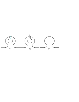
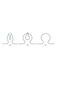
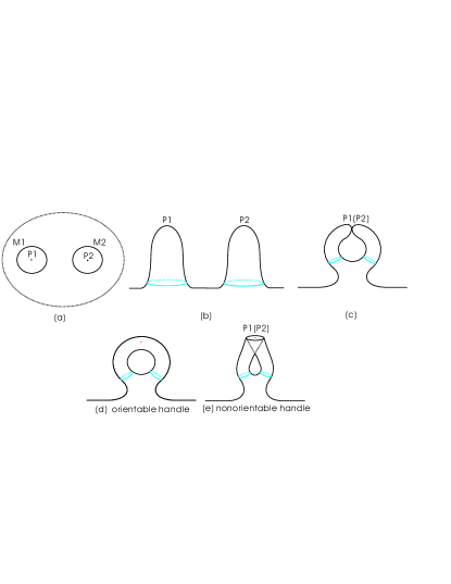
Figure 2: Extending the surface dynamics throughout a solid handle

Now let us see some examples.

Example 3.1

A single pendulum is given by the following dynamical equations

$$\dot{\theta} = {\omega}$$

$$\dot{\omega} = -\frac{g}{l}\sin{\theta}$$

Fig 3.(a) gives the dynamics in the phase-plane.

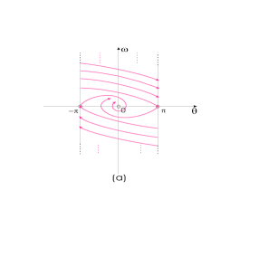
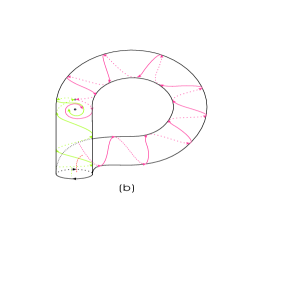
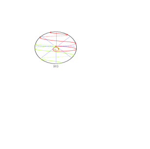
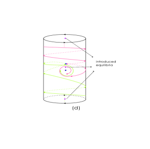
Figure 3: Extending the dynamics through Klein bottle

By identifying $-\pi$ and $\pi$ and then gluing the two ends together, we know that a pendulum is defined on a Klein bottle (see Fig 3.(b))

Next open the nonorientable handle as stated in Fig 2 from Theorem(3.1), the surface dynamics can be effectively extended throughout the 3-ball (Fig 3.(c)). Then after pulling and expanding the two poles, (as shown in Fig 3.(d)), we can glue the two ends back together and recover the Klein bottle. This time the system is situated on the whole solid Klein bottle with the surface dynamics stay unchanged.

From Proposition(2.1), we know that there is exactly one nonorientable 3-manifold with a genus $1$ Heegaard Splitting, and since Klein bottle is a nonorientable genus $1$ surface, the identity map will certainly be the homeomorphism that glues the two of them together. So in our pendulum case, there will be exactly two same systems defined on the solid Klein bottle in the above way, and via the Heegaard diagram, these two 3-manifolds will be glued by the identity map obtaining a nonorientable 3-manifold.

Example 3.2

As shown in [Banks, 2002], a surface of genus $2$ can only carry two distinct knot types. Fig 4 gives us the whole procedure of transforming a simplest knot to one type of those which can be situated on a 2-hole surface by performing the C-homeomorphisms.

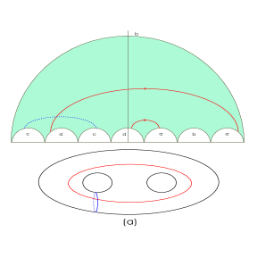
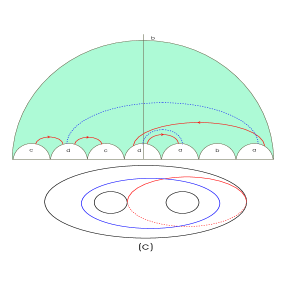
Figure 4: Transforming a simple knot to one type of the two that can be carried by a surface of genus $2$ via C-homeomorphisms

Also in [Banks & Song, 2006], we gave an explicit construction of a system that is situated on a $2$-hole torus by using the generalized automorphic functions. The system itself has Fuchsian group generated by the transformations

$$T_{1}(z) = -\frac{2z+13}{z+6}$$

$$T_{2}(z) = -\frac{1}{z+4}$$

$$T_{3}(z) = \frac{6z-13}{z-2}$$

$$T_{4}(z) = 7z-28$$

Choose

$$H_{1}(z)=\frac{1}{z+2-3i},\quad H_{2}(z)=\frac{1}{z-2-3i}$$

we obtain a system with a pole at $-2+3i$ and a zero at $2+3i$. The actual dynamics is shown in Fig 5.(a)

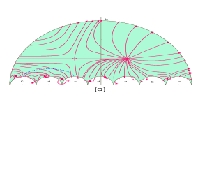
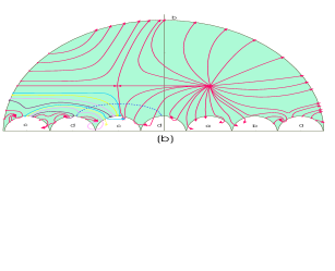
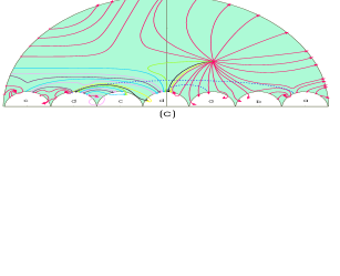
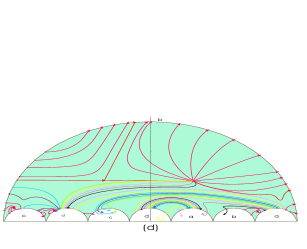
Figure 5: Change of the surface dynamics according to the C-homeomorphism surgery performed

When performing the surgery on the genus $2$ surface (as shown in Fig 4), the dynamics is also changed accordingly. Fig 5.(b)-(d) explain this procedure.

We can then extend the system throughout the solid $2$-hole torus respectively, and use the C-homeomorphisms introduced in Fig 5 to glue the surface while the matching of the dynamics is being guaranteed.

In this way, we obtain a new system which is defined on a more complicated 3-manifold from two simpler ones each sits on a solid $2$-hole torus.

4 Three-Dimensional Dynamical Systems and Heegaard Splittings

In this section we consider a three-dimensional dynamical system defined on a three-manifold without boundary containing only a finite number of equilibria. we shall examine conditions under which such a system has a Heegaard Splitting that respects the dynamics, i.e., contains an invariant genus p surface, which defines a Heegaard Splitting. Our main technical tools will be the Poincar$\acute{e}$-Hopf index theorem and the flow-box theorem. The latter may be stated as follows:

Theorem 4.1

If $\phi_{t}$ denotes a dynamical system on a manifold M of dimension n, then if $x\in M$ is not an equilibrium point (i.e., $\phi_{t}(x)\neq x,t\neq 0$), there exists a (closed) local coordinate neighbourhood U of x such that on U, $\phi_{t}$ is topological conjugate to the dynamical system

$$\left.\begin{array}[]{c}\dot{x}_{1}=c\\ \dot{x}_{2}=0\\ \vdots\\ \dot{x}_{n}=0\end{array}\right\}\quad\quad x\in\{0\leq x_{i}\leq 1,1\leq i\leq n\}$$

where c is a constant.    $\Box$

This says that locally, away from equilibria, the flow can be “parallelized”, e.g., in two dimensions the flow looks locally like the one in Fig 6.

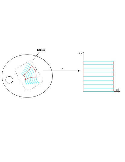
Figure 6: A local flowbox in 2-dimensional surface

Since an invariant surface in M can only have those singularities of M, in order that there exists an invariant Heegaard Splitting of genus $p\neq 1$, the dynamical system must have at least one equilibrium, so that systems with no equilibria can only have genus $1$ Heegaard Splittings, i.e., torus or Klein bottle splittings.

Theorem 4.2

In order that a 3-dimensional dynamical system on a compact manifold M has a Heegaard splitting (compatible with the dynamics) of genus p, it is necessary that it contains at least one equilibrium and that in some subset of the equilibria, ${M_{1},\cdots,M_{l}}$, there is an invariant two-dimensional local surface passing through the equilibrium with (2-dimensional) index $\vartheta_{i}$, such that

$$\sum_{i=1}^{l}\vartheta_{i}=2(1-p)\quad\quad\qquad\Box$$

Corollary 4.1

A dynamical system on a compact 3-manifold which has only linearizable equilibria and a compatible Heegaard Splitting of genus $p\geq 1$ must have at least $2(p-1)$ hyperbolic points.      $\Box$

The above necessary conditions are not sufficient, in general, to find sufficient conditions for a dynamical Heegaard Splitting we first recall the following result for a topological Heegaard Splitting and give a proof in order to motivate the generalization.

Theorem 4.3

(see [Hempel, 1976]) Every closed, connected 3-manifold M has a Heegaard Splitting.

Proof. Take a triangulation K of M and let $\Gamma_{1}$ be the set of all $1$-simplexes of K(i.e., the $1$-skeleton). Let $\Gamma_{2}$ be the dual $1$-skeleton, which is the maximal $1$-subcomplex of the first derived complex $K^{\prime}$ which is disjoint from $\Gamma_{1}$. Then if we put

$$V_{i}=N(\Gamma_{i},K^{\prime\prime})$$

where N is the normal neighbourhood of $\Gamma_{i}$ with respect to $K^{\prime\prime}$ (the second derived of K), it can be shown that $(V_{1},V_{2})$ is a Heegaard Splitting of M. $\Box$

It follows that any Heegaard Splitting can be described in this way. Suppose there is a dynamical Heegaard Splitting of a dynamical system on a closed connected manifold M. Let K be a triangulation of M determining the splitting as in Theorem(4.3). Then if $V_{i}=N(\Gamma_{i},K^{\prime\prime})$ as above, $S=V_{1}\cap V_{2}$ is a surface which is invariant under the dynamics. Since M is compact, we can cover M by a finite number of open sets $\{F_{1},F_{2},\cdots,F_{L}\}$ where $F_{i}$ is a flow box if it does not contain an equilibrium point of the dynamics or just a neighbourhood of such a point otherwise. Suppose that $\{p_{1},\cdots,p_{k}\}$ are equilibrium points of the dynamics which belong to S, and that $p_{i}\in F_{i}$ $(1\leq i\leq k)$. (This can always be done by renumbering the $F_{i}$’s.) Let

$${E_{i}}^{j}=F_{i}\cap V_{j}\quad\quad 1\leq i\leq k,1\leq j\leq 2$$

Then we can find a refinement $\{{F_{1}}^{\prime},\cdots,{F_{l_{1}}}^{\prime},{F_{1}}^{\prime\prime},\cdots,{F_{l_{2}}}^{\prime\prime}\}$ of the remaining open sets $\{F_{k+1},\cdots,F_{L}\}$ so that there exists a partition

$$\Gamma^{1}=\{E_{1}^{1},E_{2}^{1},\cdots,E_{k}^{1},{F_{1}}^{\prime},\cdots,{F_{l}}^{\prime}\}$$

$$\Gamma^{2}=\{E_{1}^{2},E_{2}^{2},\cdots,E_{k}^{2},{F_{1}}^{\prime\prime},\cdots,{F_{l}}^{\prime\prime}\}$$

such that

$$\cup\Gamma^{i}\subseteq V_{i},\quad\quad 1\leq i\leq 2$$

so that the sets $\Gamma^{1}$ and $\Gamma^{2}$ are invariant under the dynamics. By taking the flow boxes small enough, we can associate a triangulation of the manifold M (by taking the corners of the flow boxes away from the vertices) which is arbitrarily close to the original one. Clearly, conversely, if we can find a system of flow boxes for the dynamics on M with the above properties and the associated triangulation, then we will have a dynamical Heegaard Splitting. Thus we have proved

Theorem 4.4

Consider a compact 3-manifold M on which is given a compact dynamical system. Suppose there is a refinement $\Gamma^{1}\cup\Gamma^{2}$ of a covering of M by flow boxes or neighbourhoods of equilibria, such that $\Gamma^{1}$ and $\Gamma^{2}$ are invariant under the dynamics. Let $\Gamma^{1}$ and $\Gamma^{2}$ be triangulations of $\cup\Gamma^{1},\cup\Gamma^{2}$, respectively, such that $\Gamma^{1}\cup\Gamma^{2}$ is a triangulation of $M^{\prime}$. Then $(\cup\Gamma^{1},\cup\Gamma^{2})$ is a dynamical Heegaard Splitting of M if $\Gamma^{1}$ and $\Gamma^{2}$ are dual triangulations or the two-skeletons of $\Gamma^{1}$ and $\Gamma^{2}$ have equal Euler characteristics.   $\Box$

5 Connected Sums

Connected Sums of 2- and 3-manifolds provide an effective means of generating ‘complicated’ manifolds out of simpler ones. In this section we shall consider sums of dynamical systems on 2- and 3-manifolds.

Consider first the case of 2-manifolds. Given two (topological) 2-manifolds $S_{1}$ and $S_{2}$, their connected sum $S_{1}\#S_{2}$ is obtained by removing discs $D_{1}$, $D_{2}$ from $S_{1}$ and $S_{2}$ and sewing $S_{1}/S_{2}$ to $S_{2}/D_{2}$ along the boundaries of the discs. If $S_{2}$ is a sphere, note that

$$S_{1}\#S_{2}=S_{1}$$ (3)

Lemma 5.1

Let $S_{1}$ and $S_{2}$ be two surfaces on which dynamical systems $\phi_{1}$ and $\phi_{2}$ are defined. If we form the connected sum by removing discs $D_{1}$, $D_{2}$ from $S_{1}$ and $S_{2}$ away from any critical points, then we must introduce two hyperbolic equilibria (with index $-1$) on the disc boundaries.

Proof. Since there are no equilibrium points in the discs being removed, we can find flow boxes $F_{1}$ and $F_{2}$ in $S_{1}$ and $S_{2}$, respectively, so that

$$D_{i}\leq F_{i},\quad\quad i=1,2$$

provided $D_{1},D_{2}$ are small enough. The discs can be chosen so that there are two trajectories which are tangent to the discs at two points. (see Fig 7)

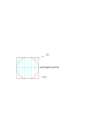
Figure 7: Trajectories in flow box $F_{1}$ tangent to disc $D_{1}$

If we now pull out tubes to form the connected sum S, these two points clearly become singular points on the connected sum as in Fig 8.

Figure 8: Change to the dynamics after gluing two tori via Connected Sum

Suppose that one surface, say $S_{2}$, is a sphere. Since $S=S_{1}\#S_{2}=S_{1}$ in this case and $\chi(S_{2})=2$, the total index of the two singular points on the removed discs must be $-2$.   $\Box$

Suppose next that we form a connected sum by removing discs containing equilibria. There are several conditions that we have to consider.

Lemma 5.2

If we form the connected sum of two surfaces $S_{1},S_{2}$ by removing discs $D_{1}$ and $D_{2}$, which each contain an equilibrium $p_{i}(i=1,2)$ without introducing new equilibria, then these equilibria must be ‘dual’ in the sense that if one equilibrium has $n_{1}$ elliptic sectors and $n_{2}$ hyperbolic sectors, then the other must have $n_{1}$ hyperbolic sectors and $n_{2}$ elliptic ones.

Proof. Again we can assume $S_{2}$ is a sphere without loss of generality. Let

$$S=S_{1}\#S_{2}=S_{1}$$

so that

$$\chi(S)=\chi(S_{1})$$

The index of one equilibrium point is

$$I(p_{1})=1+\frac{n_{1}-n_{2}}{2}$$

Since $\chi(S_{2})=2$, and without introducing extra equilibria, $p_{2}$ must have index satisfying

$$I(p_{2})+I(p_{1})=2$$

so that

$$I(p_{2})=2-I(p_{1})=1+\frac{n_{2}-n_{1}}{2}.\quad\quad\Box$$

Also, after removing discs containing equilibria and gluing the rest together, we may introduce extra critical points on the disc boundaries as well.

Lemma 5.3

Stick to the same notations as in Lemma(5.2), if there are new equilibria being introduced, and the structure of $p_{1}$ and $p_{2}$ are exactly the same, (i.e., $p_{1}$ and $p_{2}$ both have $n_{1}$ elliptic sectors and $n_{2}$ hyperbolic sectors,) then the introduced equilibria must be $n_{1}$ elliptic (with index $+1$) and $n_{2}$ hyperbolic (with index $-1$).

Proof. Without loss of generality,we first look at the case of a hyperbolic equilibrium (with index $-1$). It has $4$ hyperbolic sectors. The removed discs $D_{1}$ and $D_{2}$ can be chosen such that there are exactly four trajectories tangent to the discs at four different points, as shown in Fig 9.(A) .

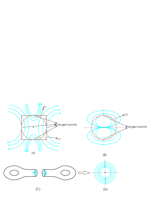
Figure 9: Gluing two tori while introducing extra equilibria

The same argument in the proof of Lemma(5.1) applies here. Referring to Fig 8, one hyperbolic sector generates one hyperbolic equilibrium (with index $-1$) after the gluing. And since $p_{i}$ has $n_{2}$ hyperbolic sectors, we end up with $n_{2}$ hyperbolic equilibria (all with index $-1$ respectively) being introduced after the gluing via connected sum.

We next consider the elliptic sectors. Suppose $p_{1}$ and $p_{2}$ only contain $n_{1}$ elliptic sectors, as shown in Fig 9.(B), within an elliptic sector, it is always possible to find two closed elliptic trajectories which are tangent to discs $D_{1}$ and $D_{2}$, respectively. If we then pull out tubes to form the connected sum S, these two points will certainly turn into two singular points on the sphere, which are elliptic equilibria and contain cycles only. (See Fig 9.(C) and (D)).

Still, we let $S_{2}$ be a sphere and

$$S=S_{1}\#S_{2}=S_{1}$$

such that

$$\chi(S)=\chi(S_{1})=m$$

also we have

$$I(p_{1})=I(p_{2})=1+\frac{n_{1}}{2}$$

Suppose there are $n$ elliptic equilibria (with index $1$) being introduced after the gluing, and since $\chi(S_{2})=2$, we have

$$m-(1+\frac{n_{1}}{2})+2-(1+\frac{n_{1}}{2})+n=m$$

which gives us $n=n_{1}$. So there are $n_{1}$ new elliptic equilibria appearing in $S$.     $\Box$

Certainly, the structure of $p_{1}$ can be different from $p_{2}$ even if there are extra equilibria being introduced.

Lemma 5.4

If we form the connected sum of two surfaces $S_{1},S_{2}$ via removing discs $D_{1}$ and $D_{2}$ which each contain an equilibrium $p_{i}(i=1,2)$, then there must exist a separation to the sectors in $p_{1}$: $n_{11}$ elliptic and $n_{21}$ hyperbolic sectors share the same structure as those in $p_{2}$, while the rest are ‘dual’ to the remaining in $p_{2}$.

Proof. The proof follows from those of Lemma(5.2) and (5.3) since these two are the only conditions that can happen to the dynamics situated on surfaces when performing the connected sum. Separate $n_{1}$ elliptic sectors of $p_{1}$ to $n_{11}$ and $n_{12}$, $n_{2}$ hyperbolic ones to $n_{21}$ and $n_{22}$, with $n_{11}$ and $n_{21}$ being attached to the same structure on $p_{2}$, while $n_{12}$ and $n_{22}$ being glued to their ‘dual’ respectively.

Again, without loss of generality, we assume one surface, $S_{2}$, is a sphere such that $\chi(S_{2})=2$ and $S=S_{1}\#S_{2}=S_{1}=m$. And since

$$I(p_{1})=1+\frac{n_{1}-n_{2}}{2}=1+\frac{n_{11}+n_{12}-n_{21}-n_{22}}{2}$$ (4)

$$I(p_{2})=1+\frac{n_{11}+n_{22}-n_{21}-n_{12}}{2}$$ (5)

From Equation(4), (5) and Lemma(5.3),

$$m-I(p_{1})+2-I(p_{2})+n_{11}-n_{21}=m$$

is satisfied.     $\Box$

We now extend the above results to the three-dimensional case. In this case, the connected sum of two compact 3-manifolds $M_{1},M_{2}$ is defined by removing two 3-cells from $M_{1}$ and $M_{2}$ and attaching their (spherical) boundaries together. This time, the Euler Characteristic of a compact 3-manifold is $0$, so by $Poincar\acute{e}$-$Hopf$ theorem, the total index of any vector field on the manifold is $zero$. First we form a connected sum by removing 3-cells which contain no equilibria. This time the singular set is a (topological) circle, so we must introduce an infinite set of equilibria or a limit cycle - we can do this by twisting the cells before gluing. Note that the cycle does not change the index, as expected. If we perform the connected sum by removing cells containing equilibria without introducing new singularities, then the equilibria must be ‘dual’ in the sense that regions on one part which point out of the cell must be matched by those on the other part which point inwards. Clearly, the indices of such critical points in 3-dimensions are the inverse of each other, going a total index change of $0$, again as expected by the $Poincar\acute{e}$-$Hopf$ theorem. If during the procedure of removing 3-cells containing critical points, we introduce new singularities, then from the combination of the statements above, we know the total change of index is still $zero$.

6 Conclusions

In this paper, we have show how to generate a new dynamical system on a complicated 3-manifold from a given one situated on a much simpler 3-manifold by considering the corresponding Heegaard diagram, C-homeomorphisms and the resulting dynamics on the boundaries. Also, we gave the sufficient conditions under which a system, which is defined on a three-manifold without boundary while containing only a finite number of equilibria, has a Heegaard Splitting which respects the dynamics. A deeper look at Connected Sum and its effect on the natural dynamics will be taken in the future paper.

References

- [1] Banks, S. P. and Song, Y. [2006] “Elliptic and automorphic dynamical systems on surfaces”, Int. J. of Bifurcation and Chaos, in press.
- [2] Banks, S. P. [2002]“Three-dimensional stratifications, knots and bifurcations of two-dimensional dynamical systems”, Int. J. of Bifurcation and Chaos, 12, No. 1, 1-21.
- [3] Hempel, J. [1976] “3-Manifolds”, Princeton University Press.
- [4] Lickorish, W. B. R. [1962] “A representation of orientable combinatorial 3-manifolds”, Ann. of Math. 76(1962), 531-540.
- [5] Ohtsuki, T. [2001] “Quantum invariants - A study of knots, 3-manifolds, and their sets”, World scientific, Series on knots and everything - Vol. 29.
- [6] Lozano, M. T. and Montesinos-Amilibia [1997] “Geodesic flows on hyperbolic orbifolds, and universal orbifolds”, Pacific J. of Mathematics, Vol. 177, No. 1.