Automorphic Forms and Reeb-Like Foliations on Three-Manifolds

Abstract

In this paper, we consider different ways of generating dynamical systems on 3-manifolds. We first derive explicit differential equations for dynamical systems defined on generic hyperbolic 3-manifolds by using automorphic function theory to uniformize the upper half-space model. It is achieved via the modification of the standard Poincaré theta series to generate systems invariant within each individual fundamental region such that the solution trajectories match up on the appropriate sides after the identifications which generate a hyperbolic 3-manifold. Then we consider the gluing pattern in the conformal ball model. At the end we shall study the construction of dynamical systems by using the Reeb foliation.
Key words:Automorphic functions, hyperbolic manifolds, upper half-space model, Poincaré theta series, conformal ball model, Reeb foliation, Heegaard splittings.

1 Introduction

Nonlinear dynamical systems are defined globally on manifolds. Consider a system

$$\dot{x}=Ax$$ (1)

where $x\in\mathbb{R}^{n}$. The phase-space portrait of this system is defined as all the solution curves in $\mathbb{R}^{n}$ (see, e.g., [Perko, 1991].) Geometrically, these curves determine the motion of all the points in the space under this specific dynamical system.

Moreover, the global manifold on which a system is stratified can be reached by studying the phase-space portrait. For example, given a spherical pendulum (see fig. 1 for illustration), it has two degrees of freedom, and the Lagrangian for this system is

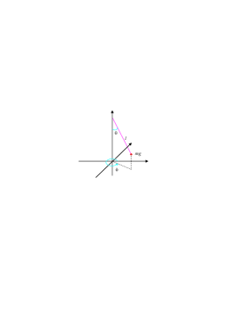
Figure 1: A spherical pendulum

$$L=\frac{1}{2}m\big{(}l^{2}{\dot{\theta}}^{2}+l^{2}(\sin{\theta})^{2}{\dot{\phi}}^{2}\big{)}+mgl\cos{\theta}.$$ (2)

The Euler-Lagrange equations give

$$\left\{\begin{array}[]{l}\frac{d}{dt}(ml^{2}\dot{\theta})-ml^{2}\sin{\theta}\cos{\theta}{\dot{\phi}}^{2}+mgl\sin{\theta}=0\\ \frac{d}{dt}\big{(}ml^{2}({\sin{\theta}})^{2}\dot{\phi}\big{)}=0\end{array}\right.$$ (3)

so the system is given by two equations of motion, i.e.,

$$\left\{\begin{array}[]{l}\ddot{\theta}={\dot{\phi}}^{2}\sin{\theta}\cos{\theta}-g/l\cdot\sin{\theta}\\ \ddot{\phi}=-({2\cos{\theta}\cdot\dot{\theta}\cdot\dot{\phi}})/{\sin{\theta}}\end{array}\right.$$ (4)

In phase-space coordinates, if set $x_{1}=\theta$, $x_{2}=\dot{\theta}=\omega_{\theta}$, $x_{3}=\phi$, $x_{4}=\dot{\phi}=\omega_{\phi}$, we then have

$$\left\{\begin{array}[]{l}\dot{x}_{1}=x_{2}\\ \dot{x}_{2}={x_{4}}^{2}\sin{x_{1}}\cos{x_{1}}-g/l\cdot\sin{x_{1}}\\ \dot{x}_{3}=x_{4}\\ \dot{x}_{4}=-({2\cos{x_{1}}\cdot x_{2}\cdot x_{4}})/{\sin{x_{1}}}\end{array}\right.$$ (5)

This is a 4-dimensional system. Now assume $x_{3}={\phi}=k$, where k is a constant, consequently $\dot{x}_{3}=0$ and ${\dot{x}}_{4}={\dot{\omega}}_{\phi}=0$, the system will then become

$$\left\{\begin{array}[]{l}\dot{x}_{1}=x_{2}\\ \dot{x}_{2}=-g/l\cdot\sin{x_{1}}\\ \dot{x}_{3}=0\\ \dot{x}_{4}=0\end{array}\right.$$ (6)

which stands for a single pendulum that sits on a 2-dimensional plane. It is known that this system is defined on a Klein bottle, (see [Banks & Song, 2006] and fig. 2 for an illustration.)

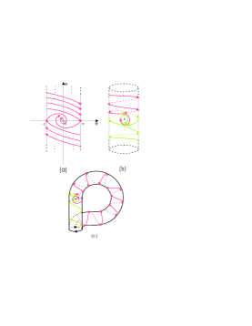
Figure 2: A single pendulum is defined on a Klein bottle

If set ${\dot{x}}_{3}=\omega_{\phi}=k$, i.e., the system has a fixed angular velocity in $\phi$, the system then becomes

$$\left\{\begin{array}[]{l}\dot{x}_{1}=x_{2}\\ \dot{x}_{2}={x_{4}}^{2}\sin{x_{1}}\cos{x_{1}}-g/l\cdot\sin{x_{1}}\\ \dot{x}_{3}=k\\ \dot{x}_{4}=0\end{array}\right.$$ (7)

which is essentially a 3-dimensional hyperplane given by $x_{4}=k$ within the 4-dimensional space. Moreover, since the vector field is periodic in both $x_{1}$ and $x_{3}$ with period $2\pi$, it is naturally defined within the cube

$$C:\{(x_{1},x_{2},x_{3}):-\pi\leq x_{1}\leq\pi,-\infty<x_{2}<\infty,$$

$$-\pi\leq x_{3}\leq\pi\}$$

as shown in fig. 3(a).

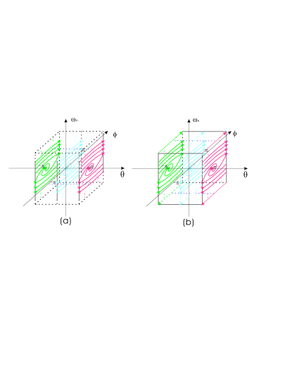
Figure 3: Phase-plane portrait of the spherical pendulum when $\omega_{\phi}=k$

Note that the phase-space portrait is a 2-dim single pendulum that sits on different slices defined by $\phi=k$, and because we know that $\theta,\phi=\pi$ and $\theta,\phi=-\pi$ are physically the same respectively, we can identify them by pairing the opposite sides via translation.

In order to define the system on a compact manifold, we compress the infinite cube to a finite one, as shown in fig. 3(b), and since the dynamics at the two ends are pointing the opposite directions, the identification will result in a self-intersection in the 3-dimensional Euclidean space, fig. 4 shows an embedding in $\mathbb{R}^{3}$.

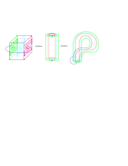
Figure 4: Construction of a 3-dimensional solid Klein bottle

Thus, we obtain the 3-manifold on which this special spherical pendulum is defined. We call it 3-dimensional solid Klein bottle.

In [Banks & Song, 2006], we showed that a dynamical system on a two-dimensional surface is given by a generalized automorphic function F. In this paper, we will extend the previous result and propose to show how to generalise explicit differential equations that naturally have global behaviour on 3-manifolds. Again we will use the theory of automorphic functions to achieve it.

2 Geometric 3-Manifolds

We shall now give a brief resumé of 3-manifolds which will be needed in the following sections. Note that all the results are well-known, for example in [Ratcliffe, 1994].

Definition 2.1

A $3$-manifold M without boundary is a $3$-dimensional Hausdorff space that is locally homeomorphic to $\mathbb{E}^{3}$,i.e., for every point $x$ $(x\in M)$ there exists a homeomorphism that maps a neighbourhood A of x onto the $3$-dimensional Euclidean space; while if M has a boundary, then the homeomorphism maps A onto the upper-half $3$-dimensional Euclidean space  $\overline{\mathbb{U}^{3}}=\{x\in\mathbb{E}^{3}:x_{3}\geq 0\}$.

Equivalently, a 3-manifold M is called a geometric 3-space. Assume that $\Gamma$ is a group which acts on a 3-dimensional geometric space X, then

Definition 2.2

The orbit space of the action $\Gamma$ on $X$ is the set of $\Gamma$–orbits,

$$X/\Gamma=\{\Gamma_{X}:x\in\Gamma\},$$

with the metric topology being the quotient topology, and the quotient map given by

$$\pi:X\to X/\Gamma.$$

Moreover, if $\Gamma$ is a discrete group of isometries of X, then $\Gamma$ is discontinuous and called a 3-dimensional Fuchsian group. In fact, it defines a fundamental region F of X which, together with its congruent counterparts, generates a tessellation of X.

Definition 2.3

For a discrete group $\Gamma$ of isometries of a geometric space X, a subset F of X is a fundamental region if and only if

1. the set F is open in X;

2. the members of $\{gF:g\in\Gamma\}$ are mutually disjoint;

3. $X=\cup\{g\overline{R}:g\in\Gamma\}$

For example, let $\tau_{i}$ be the translation of $\mathbb{E}^{3}$ by $e_{i}$ for $i=1,2,3$, then $\{\tau_{1},\tau_{2},\tau_{3}\}$ defines a discrete subgroup $\Gamma_{a}$ of $I(\mathbb{E}^{3})$. A fundamental region for $\Gamma_{a}$ will be the open unit cube in $\mathbb{E}^{3}$, as shown in fig. 5, in fact, $\Gamma_{a}$ generates a tessellation of $\mathbb{E}^{3}$.

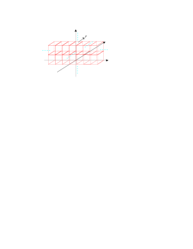
Figure 5: Tessellation of $\mathbb{E}^{3}$ by $\Gamma_{a}$ generated via translation $e_{i}$

If $\Gamma$ acts freely on X, the orbit space $X/\Gamma$ is then a 3-manifold which can also be called an X-space-form. Also, by assuming G is a group of similarities of a 3-dimensional geometric space X and M is a 3-manifold, we have

Definition 2.4

An $(X,G)$–atlas for M is a group of maps

$$\Phi=\{\phi_{i}:U_{i}\to X\}_{i\in\mathcal{I}}$$

such that:

1. The set $U_{i}$ is an open connected subset of M for each i.

2. $\phi_{i}$ maps $U_{i}$ homeomorphically onto an open subset of X for each i.

3. $\bigcup_{i\in\mathcal{I}}U_{i}=M$

4. If $U_{i}$ and $U_{j}$ overlap, then the map

   $$\phi_{j}\phi_{i}^{-1}:\phi(U_{i}\cap U_{j})\rightarrow\phi_{j}(U_{i}\cap U_{j}),$$

   agrees in a neighbourhood of each point of its domain with an element in G.

Note that $\Phi$ consists of the charts of the (X,G)–atlas. An (X,G)–structure is then defined as the maximal (X,G)–atlas for M. Hence a 3-manifold M with an (X,G)–structure is called an (X,G)–manifold. It is well-known (e.g., [Ratcliffe, 1994]) that the orbit space $X/\Gamma$, together with the induced $(X,\Gamma)$–atlas, is an $(X,\Gamma)$-manifold. Furthermore, we can obtain this 3-manifold by gluing one fundamental region F along the corresponding sides.

Let $\mathcal{F}$ be a family of fundamental regions in a geometric space X and $\Gamma$ be a group of isometries of X. We can then construct the $(X,\Gamma)$–manifold by applying the $\Gamma$-side-pairing.

Definition 2.5

A $\Gamma$-side-pairing for $\mathcal{F}$ is a subset of  $\Gamma$,

$$\Gamma=\{\tau_{s}:\textrm{S is a side of one fundamental region in}~{}\mathcal{F}\},$$

such that for each side S in $\mathcal{F}$,

1. there exists a side $S^{\prime}$ in $\mathcal{F}$ that satisfies $\tau_{s}(S^{\prime})=S$,

2. $\tau_{s^{\prime}}=\tau_{s}^{-1},$

3. if S is a side of F in $\mathcal{F}$ and ${S^{\prime}}$ is a side of ${F^{\prime}}$, then

   $$F\cap g_{s}(F^{\prime})=S.$$

The elements of $\Gamma$ are called the side-pairing transformations of $\mathcal{F}$, which generates an equivalence relation on the set $\prod=\bigcup_{F\in\mathcal{F}}F$, i.e., the cycles of $\Gamma$. Moreover, $S^{\prime}$ is uniquely determined by $S$. So if the $\Gamma$-side-pairing is proper, i.e., each cycle of $\Gamma$ is finite and has solid angle sum $4\pi$, then by choosing two fundamental regions in $\mathcal{F}$, say $F$ and $F^{\prime}$, the elements in $\Gamma$ will associate each side in $F$ with a unique one in $F^{\prime}$, identifying the corresponding sides together will eventually generate a 3-manifold with an $(X,\Gamma)$-structure attached. For instance, as in the previous example, after pairing the opposite sides of the unit cube by translations $\Gamma$, we effectively end up with a 3-manifold M which is known as the cubical Euclidean 3-torus (see fig. 6 for illustration).

Figure 6: Construction of the cubical Euclidean 3-torus

3 Automorphic Functions and Systems on Hyperbolic 3-Manifolds

In this section we shall first give a brief resumé of automorphic functions. More details can be found in, for example, [Ford, 1929; Ratcliffe, 1994].

To denote the points in $\mathbb{R}^{3}$, we use the following coordinates:

$$\mathbb{R}^{3} = \mathbb{C}\times(-\infty,\infty)$$

$$= \{(z,r)\mid z\in\mathbb{C},r\in\mathbb{R}\}$$

$$= \{(x,y,r)\mid x,y,r\in\mathbb{R}\}$$

Also, we can think $\mathbb{R}^{3}$ as a subset of Hamilton’s quaternions $\mathcal{H}$, so a point p $(p\in\mathbb{R}^{3})$ can be expressed as a quaternion whose fourth term equals to zero, i.e.,

$$p=(z,r)=(x,y,r)=z+rj,$$

where $z=x+yi$ and $j=(0,0,1)$, then

Definition 3.1

A Möbius transformation of  ${\widehat{\mathbb{R}}}^{3}$ is a finite composition of reflections of  ${\widehat{\mathbb{R}}}^{3}$ in spheres, where  ${\widehat{\mathbb{R}}}^{3}$ is the one-point compactification of  $\mathbb{R}^{3}$, i.e.,

$${\widehat{\mathbb{R}}}^{3}=\mathbb{R}^{3}\cup\{\infty\}.$$

It is exactly the linear fractional transformations of the form

$$T=\frac{ap+b}{cp+d}.$$ (8)

where $a,b,c,d\in\mathbb{R}^{3}$ and $ad-bc\neq 0$.

A Möbius transformation is a conformal map of the extended 3-space, (i.e., Riemann 3-manifold), denoted by $\textbf{Aut}(\widehat{\mathbb{R}}^{3})$. Moreover, (8) can be represented in terms of a matrix

$$G=\left(\begin{array}[]{cc}a&b\\ c&d\\ \end{array}\right).$$ (9)

In fact there exists a group homeomorphism: $\textrm{GL}(2,\mathbb{R}^{3})\to\textbf{Aut}({\widehat{\mathbb{R}}}^{3})$ given by

$$\left(\begin{array}[]{cc}a&b\\ c&d\\ \end{array}\right)\longrightarrow T,$$

which becomes an isomorphism on the projective special linear group $\textrm{PSL}(2,\mathbb{R}^{3})$ (i.e., those elements of $\textrm{GL}(2,\mathbb{R}^{3})$ of positive determinant modulo the scalar matrices).

It is known that 3-dimensional hyperbolic space (or 3-dimensional hyperbolic manifold) is the unique 3-dimensional simply connected Riemannian manifold with constant sectional curvature $-1$ (see, e.g., [Elstrodt, 1998]). Also, since Möbius transformations are defined on Riemannian manifold, they can be used to generate a discrete group of discontinuous isometries, $\Gamma$, of the upper half-space $\mathbb{U}^{3}$, where

$$\mathbb{U}^{3}: = \mathbb{C}\times(0,\infty)$$

$$= \{(z,r)\mid z\in\mathbb{C},r>0\}$$

$$= \{(x,y,r)\mid x,y,r\in\mathbb{R},r>0\}.$$

Note that $\mathbb{U}^{3}$ is a model for hyperbolic space, so we can use $\Gamma$ to tessellate $\mathbb{U}^{3}$ and obtain a 3-manifold, M, by $\Gamma$-side-pairing either the fundamental region or a finite collection of discrete regions congruent to the fundamental region. Obviously M is with $(\mathbb{U}^{3},\Gamma)$-structure.

We shall continue using Hamilton’s quaternion $\mathcal{H}$, and the notation for points p in $\mathbb{U}^{3}$ will be the same as that in $\mathbb{R}^{3}$, only with $r>0$.

Furthermore, since we restrict attention to the upper half-space, the automorphism group becomes $\textrm{PSL}(2,\mathbb{C})$ (linear fractional transformation with complex coefficients). If T is a map of the form (8), where $a,b,c,d\in\mathbb{C}$, we have

$$T(p) = T(z+rj)$$ (10)

$$= \frac{(az+b)(\bar{c}\bar{z}+\bar{d})+a\bar{c}r^{2}}{\|cp+d\|^{2}}$$

$$+j\frac{r}{\|cp+d\|^{2}}~{}.$$

For an element $g\in\textrm{PSL}(2,\mathbb{C})$, $g\neq\pm I$ is classified as follows:

1. if $|tr(g)|=2$  &  $tr(g)\in\mathbb{R}$, T is parabolic;

2. if $|tr(g)|>2$  &  $tr(g)\in\mathbb{R}$, T is hyperbolic;

3. if $0\leq|tr(g)|<2$  &  $tr(g)\in\mathbb{R}$, T is elliptic;

To define explicit expressions for dynamical systems on M, we first need to find the so-called automorphic functions that are invariant under the elements of $\Gamma$.

By definition, an automorphic function A for the Fuchsian group $\Gamma$ is a meromorphic function generated on $\mathbb{U}^{3}$ such that

$$A\big{(}T_{i}(p)\big{)}=A(p)$$

for all $T_{i}\in\Gamma$ and $p\in\mathbb{U}^{3}$ $(p=z+rj)$.

It would be nice if the dynamics on the 3-manifold M can be defined as

$$\dot{p}=A(p),$$ (11)

where A is an automorphic function. However, since we are dealing with vector fields, the solutions generated by (11) in $\mathbb{U}^{3}$ are not $\Gamma$-invariant in the sense that dynamics at the boundary of the fundamental region won’t match up when applying the $\Gamma$-side-pairing. In order to obtain systems $\dot{p}=f(p)$ with $\Gamma$-invariant trajectories, we require the following invariance of the vector field f:

Lemma 3.1

The system

$$\dot{p}=f(p)$$

will have $\Gamma$-invariant trajectories for any given discrete group  $\Gamma$ of isometries of hyperbolic $3$-space X, if

$$f(p)=\frac{d\Big{(}T^{-1}\big{(}T(p)\big{)}\Big{)}}{dp}\cdot f\big{(}T(p)\big{)},\qquad\forall~{}T\in\Gamma.$$ (12)

Proof. To make the dynamics match up after the side-pairing, we require the “ends” of infinitesimal vectors in the direction of $f(p)$ to map appropriately under $\Gamma$ (see fig. 7 for illustration).

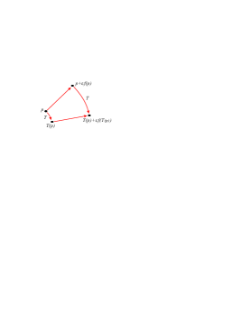
Figure 7: Mapping the vector field under any $\textit{T}\in\Gamma$

Hence we require

$$T\big{(}p+\varepsilon f(p)\big{)}=T(p)+\varepsilon f\big{(}T(p)\big{)}$$

for sufficiently small $\varepsilon$. Thus

$$f(p) = \frac{T^{-1}\Big{(}T(p)+\varepsilon f\big{(}T(p)\big{)}\Big{)}-p}{\varepsilon}$$

$$f(p) = \frac{T^{-1}\Big{(}T(p)+\varepsilon f\big{(}T(p)\big{)}\Big{)}-T^{-1}\big{(}T(p)\big{)}}{\varepsilon f\big{(}T(p)\big{)}}$$

$$\cdot f\big{(}T(p)\big{)}$$

$$\therefore\qquad f(p)=\frac{dT^{-1}}{dp}\big{(}T(p)\big{)}\cdot f\big{(}T(p)\big{)},$$

so the lemma is proved.   $\square$

To work out the relation between $f(p)$ and $f\big{(}T(p)\big{)}$ explicitly, we have, from (8),

$$T^{-1}(p)=\frac{dp-b}{-cp+a}$$

$$\therefore\qquad\frac{d}{dp}\big{(}T^{-1}(p)\big{)}=\frac{ad-bc}{(a-cp)^{2}}$$

$$\Longrightarrow\qquad\frac{dT^{-1}}{dp}\big{(}T(p)\big{)}=\frac{(cp+d)^{2}}{ad-bc}$$

Therefore, for such a map $\textit{T}\in\Gamma$, the invariance of the dynamical system f given by (12) can be written in the form

$$F\big{(}T(p)\big{)}=\frac{ad-bc}{(cp+d)^{2}}\cdot F(p)$$ (13)

Note that (13) differs from the scalar invariance

$$A\big{(}T(p)\big{)}=A(p),\qquad\textit{T}\in\Gamma,$$

which is given by any automorphic function. So we shall obtain vector fields F that satisfies (13) by modifying the Poincaré theta series (see [Ford, 1929]) which can be used to generate automorphic functions for those Fuchsian groups with infinite elements.

Definition 3.2

Let H be a rational function, which has no poles at the limit points of the isometry group $\Gamma$, the theta series is given by

$$\theta(p)=\sum_{i=0}^{\infty}(c_{i}p+d_{i})^{2}\cdot H(p_{i}),$$

where $p\in\mathbb{U}^{3}$, $I,T_{1},T_{2},T_{3},\cdots$ are the elements of  $\Gamma$, and

$$p_{i}=T_{i}(p)=\frac{a_{i}p+b_{i}}{c_{i}p+d_{i}}.$$

It is easy to verify that

$$\theta(p_{i})=(c_{i}p+d_{i})^{2m}\cdot\theta(p)$$

for each i, and by definition, two distinct theta series $\theta_{1}$ and $\theta_{2}$ with the same choice on m, we can have

$$F(p)=\frac{\theta_{1}(p)}{\theta_{2}(p)}.$$

Moreover,

$$F(p_{i})=F(p)$$

for each i, i.e., F is an automorphic function.

From (13), we know that in the case of dynamical systems, some modification must be made to the theta series so that they can provide the invariance of the vector fields. Therefore instead of  $\theta_{1}$, we define

$$\widetilde{\theta}_{1}(p)=\sum_{i=0}^{\infty}\frac{(c_{i}p+d_{i})^{2-2m}}{(a_{i}d_{i}-b_{i}c_{i})}\cdot H_{1}\big{(}T_{i}(p)\big{)}$$

while keep  $\theta_{2}(p)$ as usual.

Lemma 3.2

The function

$$F(p)=\frac{{\widetilde{\theta}}_{1}(p)}{\theta_{2}(p)}$$

satisfies

$$F\big{(}T_{i}(p)\big{)}=\frac{a_{i}d_{i}-b_{i}c_{i}}{(c_{i}p+d_{i})^{2}}\cdot F(p)$$

for each i and so defines a $\Gamma$-invariant dynamical system if $m\geq 2$.

Proof. Since $\theta_{2}$ is the normal theta series, we have

$$\theta_{2}\big{(}T_{j}(p)\big{)}=(c_{j}p+d_{j})^{2m}\cdot\theta_{2}(p)$$

for each j, while for  $\widetilde{\theta}_{1}$, we have

$$\widetilde{\theta}_{1}\big{(}T_{j}(p)\big{)} = \sum_{i=0}^{\infty}\frac{H_{1}\big{(}T_{i}T_{j}(p)\big{)}}{\Big{(}c_{i}(\frac{a_{j}p+b_{j}}{c_{j}p+d_{j}})+d_{i}\Big{)}^{2m-2}(a_{i}d_{i}-b_{i}c_{i})}$$

$$= \sum_{i=0}^{\infty}\frac{(c_{j}p+d_{j})^{2m-2}}{\big{(}(c_{i}a_{j}+d_{i}c_{j})p+c_{i}b_{j}+d_{i}d_{j}\big{)}^{2m-2}}$$

$$\cdot\frac{H_{1}\big{(}T_{i}T_{j}(p)\big{)}}{(a_{i}d_{i}-b_{i}c_{i})}$$

$$= (c_{j}p+d_{j})^{2m-2}(a_{j}d_{j}-b_{j}c_{j})\cdot$$

$$\sum_{i=0}^{\infty}\frac{1}{\big{(}(c_{i}a_{j}+d_{i}c_{j})p+c_{i}b_{j}+d_{i}d_{j}\big{)}^{2m-2}}$$

$$\cdot\frac{H_{1}\big{(}T_{i}T_{j}(p)\big{)}}{(a_{i}d_{i}-b_{i}c_{i})(a_{j}d_{j}-b_{j}c_{j})}$$

$$= (c_{j}p+d_{j})^{2m-2}(a_{j}d_{j}-b_{j}c_{j})\cdot\widetilde{\theta}_{1}(p),$$

since

$$T_{i}T_{j}(p) = \frac{a_{i}\frac{a_{j}p+b_{j}}{c_{j}p+d_{j}}+b_{i}}{c_{i}\frac{a_{j}p+b_{j}}{c_{j}p+d_{j}}+d_{i}}$$

$$= \frac{(a_{i}a_{j}+b_{i}c_{j})p+(a_{i}b_{j}+b_{i}d_{j})}{(c_{i}a_{j}+d_{i}c_{j})p+(c_{i}b_{j}+d_{i}d_{j})},$$

and

$$\textrm{det}\big{(}T_{i}T_{j}(p)\big{)} = (a_{i}a_{j}+b_{i}c_{j})(c_{i}b_{j}+d_{i}d_{j})$$

$$-(a_{i}b_{j}+b_{i}d_{j})(c_{i}a_{j}+d_{i}c_{j})$$

$$= (a_{j}d_{j}-b_{j}c_{j})\cdot(a_{i}d_{i}-b_{i}c_{i}).$$

Hence

$$F(p) = \frac{\widetilde{\theta}_{1}(p)}{\theta_{2}(p)}$$

$$= \frac{\frac{1}{(c_{j}p+d_{j})^{2m-2}(a_{j}d_{j}-b_{j}c_{j})}\cdot\widetilde{\theta}_{1}\big{(}T_{j}(p)\big{)}}{\frac{1}{(c_{j}p+d_{j})^{2m}}\cdot\theta_{2}\big{(}T_{j}(p)\big{)}}$$

$$= \frac{(c_{j}p+d_{j})^{2}}{a_{j}d_{j}-b_{j}c_{j}}\cdot F\big{(}T_{j}(p)\big{)}$$

$$= \big{(}(T_{j})^{-1}\big{)}^{\prime}\big{(}T_{j}(p)\big{)}\cdot F\big{(}T_{j}(p)\big{)},$$

therefore the result follows.   $\Box$

Definition 3.3

An automorphic vector field on $\mathbb{U}^{3}$ is a meromorphic, hypercomplex valued function F, such that it satisfies (13) for each isometry T in the Fuchsian group $\Gamma$.

From the discussion above, we know that such functions F, generate dynamics situated on hyperbolic 3-manifolds, which is written in the form

$$\dot{p}=F(p).$$

The trajectories are $\Gamma$-invariant on any fundamental region, we can then either “wrap up” one of them or choose a finite number and apply the $\Gamma$-side-pairing, both of which will give rise to systems sit on the resulting hyperbolic 3-manifold explicitly.

Example. It is known that the upper half-space $\mathbb{U}^{3}$ can be tessellated by hyperbolic ideal tetrahedron. Fig. 8 shows one particular representation.

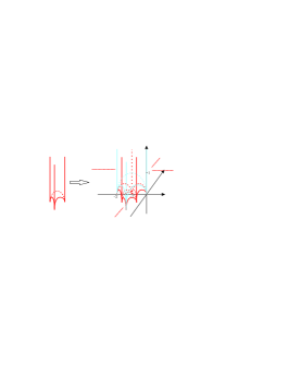
Figure 8: Tessellation of $\mathbb{U}^{3}$ by hyperbolic tetrahedra

Let the $\Gamma$-side-pairing be either translations or simple expansions and contractions. According to fig.8 we then have the Fuchsian group generated by the transformations

$$\begin{array}[]{ll}T_{1}(p)=\frac{p-2}{2};&\qquad T_{2}=\frac{p}{2};\\ T_{3}(p)=\frac{p-1-\sqrt{3}i}{2};&\qquad T_{4}(p)=\frac{p+3+{\sqrt{3}}i}{2};\\ T_{5}(p)=p+2.\end{array}$$

Choosing

$$H_{1}(p)=p+\frac{1}{2}+\frac{\sqrt{3}}{2}i+5j,\qquad H_{2}(p)=1.$$

We can obtain a dynamical system by using the modified automorphic functions. Note that in this example, $H_{1}$ and $H_{2}$ don’t define poles within the phase-space, however, the system will have poles introduced by the modified theta series. In fact, the whole z–plane will be covered with equilibria due to the fact that it contains only cusp points. Fig. 9 shows one possible construction of a hyperbolic 3-manifold by translation. Moreover, fig. 10 illustrates the solution trajectories of the system (computed in MAPLE), and the vector fields match up perfectly at the boundaries.

Figure 9: Side-pairing two tetrahedra by translation

Figure 10: The solution trajectories for the system $\dot{p}=F(p)$, where F is generated by $H_{1}$ and $H_{2}$.

4 Gluing 3-Manifolds Using the Conformal Ball Model

We now propose another way of generating dynamical systems on 3-manifolds. Instead of using the upper half-space model, we shall now investigate hyperbolic 3-manifolds under the conformal ball model. The same argument applies here, i.e., given a group $\Gamma$ of isometries of $X$ and a proper $\Gamma$-side-pairing, we can form a 3-manifold $M$ with an $(X,\Gamma)$-structure by gluing a finite number of disjoint convex polyhedra. Moreover, if we take into consideration of the dynamical systems naturally situated on those solid fundamental polyhedra, the $\Gamma$-side-pairing will then yield a new system defined on the resulting manifold $M$ if and only if the trajectories match up according to the gluing pattern.

Again, as an example, we consider a regular ideal tetrahedron in $B^{3}$, which has the shape in fig. 11.

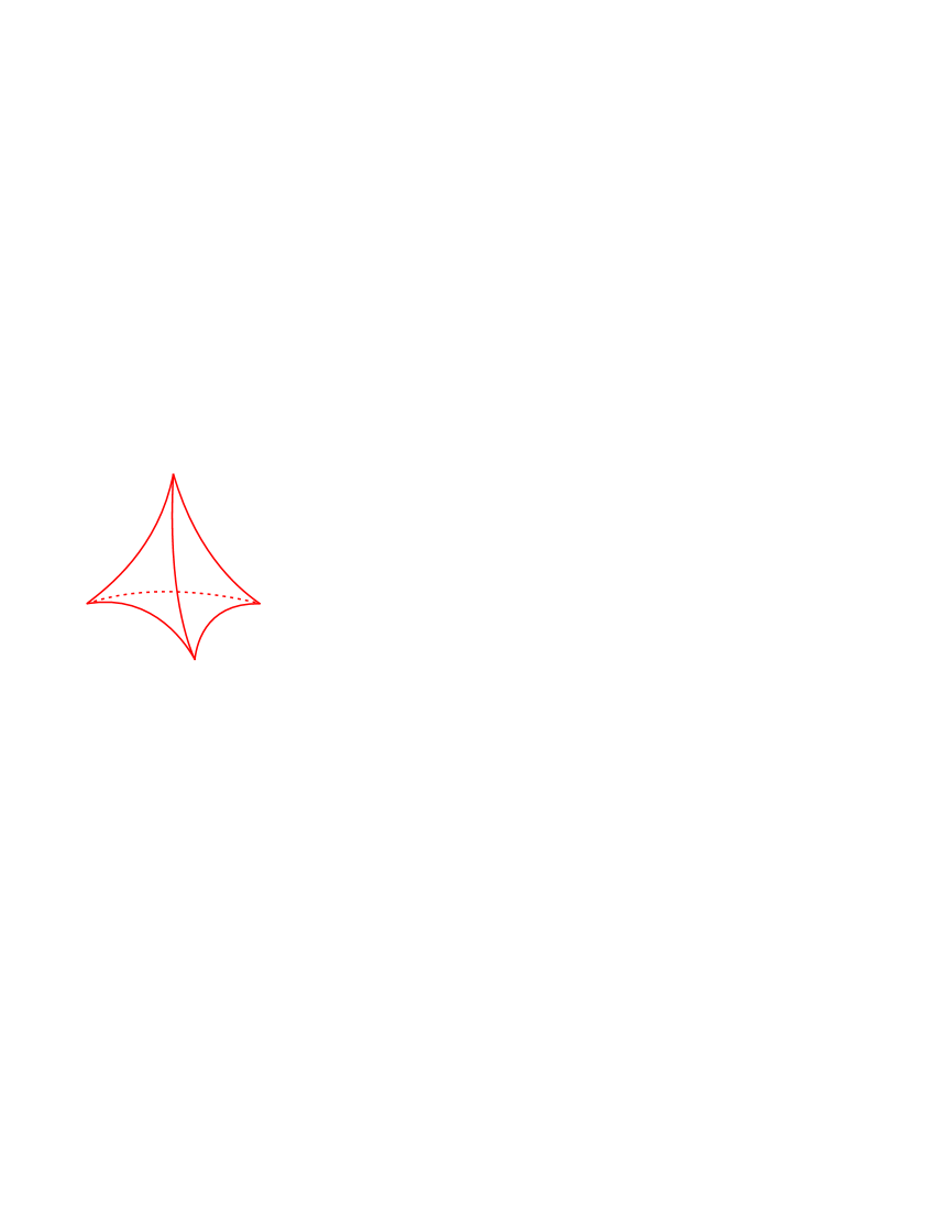
Figure 11: An ideal tetrahedron

Let $T_{1}$ and $T_{2}$ be two disjoint regular ideal tetrahedrons in $B^{3}$, illustrated in fig. 12. For simplification, we regard them as regular tetrahedrons in the Euclidean space.

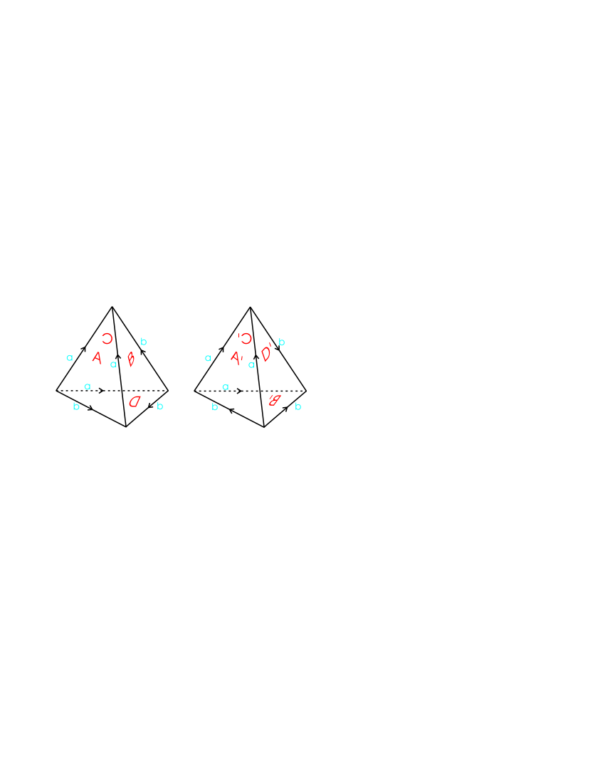
Figure 12: The gluing pattern of two regular ideal tetrahedrons

Because a Möbius transformation of the unit ball $B^{3}$ leaves it invariant, the permutation of the four vertices will determine the gluing pattern accordingly. If we label the sides and edges of $T_{1}$ and $T_{2}$ as in fig. 12, there must exist an isometry of $B^{3}$ such that the sides of $T_{2}$, namely, $A^{\prime}$, $B^{\prime}$, $C^{\prime}$, $D^{\prime}$, are mapped onto those of $T_{1}$, i.e., $A$, $B$, $C$, $D$, and exactly in this order. It can be proved that this side-pairing is proper, hence implies that the resulting space will be a hyperbolic 3-manifold, say $M$, which is known as the figure-eight knot complement.

Now by assuming the existence of systems on these solid regular tetrahedrons, a new dynamical system can then be constructed on the resulting manifold via the side-pairing if and only if the trajectories match up on the corresponding boundaries of the polyhedra components. As an example, fig. 13 illustrates this matching up by applying the side-pairing that we mentioned above. Note that the explicit dynamics in (a) and (c) are obtained by repeating (b) and (d) on all sides and edges of $T_{1}$ and $T_{2}$, respectively.

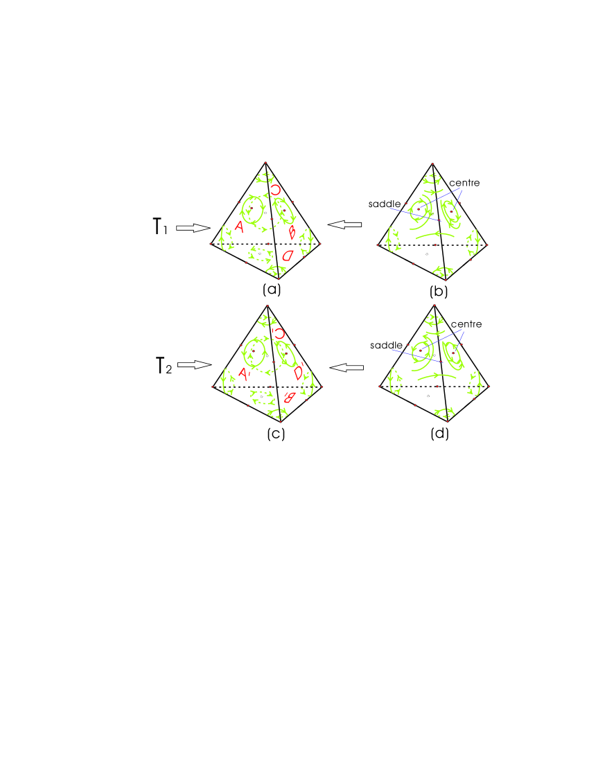
Figure 13: Dynamical systems on T1 and T2

5 Modified Reeb Foliations and Systems on 3-Manifolds

The classical Reeb foliation of the sphere and the torus are well-known (see [Moerdijk & Mrcun, Candel & Conlon, 2000]). These are obtained first from a Heegaard splitting of the sphere

$$S^{3}\cong X\cup_{\partial X}X$$

where $X$ is a solid torus and each copy of $X$ carries the foliation shown below in fig. 14.

Figure 14: The Reeb Foliation.

Each leaf apart from the bounding torus is a plane immersed into the solid torus. In this paper we shall show that an infinite set of dynamical systems exists on the 3-sphere which are formed by taking a genus $p$ (for any $p\geq 1$) Heegaard Splitting of $S^{3}$ and finding a generalized Reeb foliation on the solid genus $p$ bounded 3-manifolds. Each leaf (apart from the bounding genus $p$ surfaces and a singular leaf) will be an unbounded surface of infinite genus. Of course, it is well-known that every compact three-manifold has a (nonsingular) foliation (see [Candel & Conlon, 2000]), essentially proved by Dehn surgery on embedded tori, each of which carries a Reeb component. However, this is an existence result and it is difficult to use to define explicit dynamical systems on three-manifolds.

We begin by describing a simple system on the torus which can be mapped onto each leaf of the Reeb foliation to give a system on $\mathbb{R}^{2}$ with an infinite number of equilibria. The basic system on the torus will consist of a source, a sink and two saddles as shown in fig. 15.

Figure 15: A Simple system on the torus

(Note that the converse of the Poincar$\acute{e}$ index theorem is not true, so it is not possible to have just a source and a saddle on the torus, although their total index would be $0$.) Consider a single noncompact leaf in the Reeb foliation consisting of a ‘rolled up’ plane as in fig. 16,

Figure 16: A single leaf $L$

The plane $P$ cuts the leaf $L$ into an infinite number of cylinders plus a disk. Mapping the dynamics of fig. 15 onto each cylinder and adding a source at the origin of the disk gives the system on the plane shown in fig. 17.

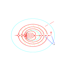
Figure 17: Resulting dynamics on the cylinder

We shall organize the dynamics on the leaf so that the sources lie ‘below’ the point $x$ on the torus when the leaf is folded up.

Note that the size of the shaded region in fig. 17 depends on the leaf and shrinks to zero with origin ‘below’ $x$ as in fig. 18.

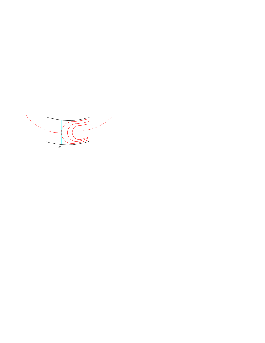
Figure 18: Shrinking of the leaf

We shall now show that there is a (singular) foliation of a 3-manifold of genus $p$ containing a compact leaf consisting of the bounding genus $p$ surface, an uncountable number of unbounded leaves of infinite genus and a set of one-dimensional singular leaves. Consider first the genus $2$ case.

Lemma 5.1

Consider the orientable $3$-manifold with boundary consisting of the closed surface of genus $2$. There is a singular foliation of this manifold defined by a dynamical system with a singular one-dimensional invariant submanifold, an infinite number of noncompact invariant submanifolds of infinite genus and a single leaf consisting of the boundary.

Proof. We obtain the foliation by modifying the Reeb foliation and its associated dynamical system introduced above. Hence consider two systems of the form in fig. 17, where one has the arrows reversed (i.e. we reverse time in the corresponding dynamical system). We then form the connected sum of the bounding tori by removing a disk around the source (or sink) at the point $x$. Then we ‘plumb’ each leaf in a similar way (again removing the source or sink). This will require one singular line joining the origins of the leaves which occur just ‘below’ $x$. See fig. 19 for illustration.

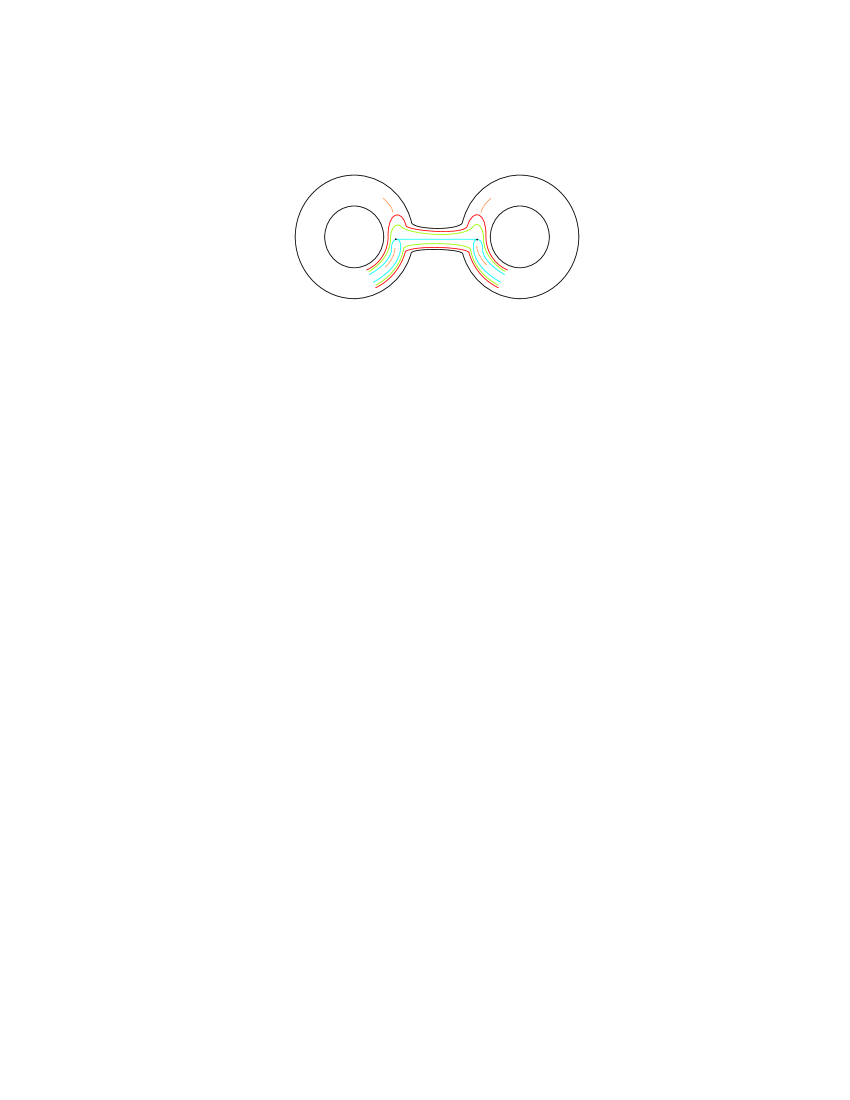
Figure 19: Gluing two tori via the leaves

The leaves clearly have the form stated in the lemma.   $\Box$

Remarks. The nonsingular leaves (apart from the genus $2$ boundary surface) are embeddings of the surfaces shown in fig. 20.

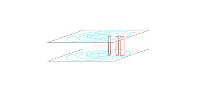
Figure 20: A typical leaf

Note that we must have at least one singular fibre in order to introduce such a foliation on a higher genus surface. For we have

Theorem 5.1

Any foliation of codimension $1$ of a compact orientable manifold $M$ of dimension $3$ with finite fundamental groups and genus $>1$, which is transversally oriented, must have a singular leaf.

Proof. By Novikov’s theorem (see [Moerdijk & Mrcun, 2003]), any codimension $1$ transversely orientable foliation of $M$ has a compact leaf and if $M$ is orientable, this compact leaf is a torus containing a Reeb component. Thus, if $M$ contains a compact leaf of genus $>1$, it is not a torus and hence there must exist a singular leaf.   $\Box$

Remarks. We can find a similar singular foliation of a genus $2$ 3-manifold by adding a handle between the stable and unstable points on the torus in fig. 15. This gives a typical leaf shown in fig. 21, rather than the one in fig. 20.

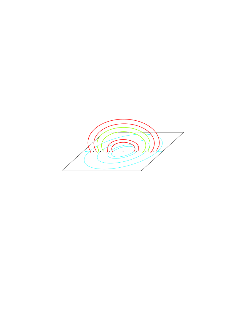
Figure 21: A typical leaf obtained by adding handles

We now define systems on 3-manifolds by gluing two systems of the form above situated on solid genus-$p$ surfaces by the use of a Heegaard diagram. We first recall the general theory of Heegaard Splittings of 3-manifolds (see, e.g. [Hempel, 1976]). A Heegaard Splitting of genus $p$ $(V_{1},V_{2})$ of a 3-manifold $M$ is a pair of solid cubes with $p$ handles $V_{1}$, $V_{2}$ such that $M$ is obtained from $V_{1}$ and $V_{2}$ by gluing $\partial V_{1}$ to $\partial V_{2}$. Using a simplicial decomposition of $M$ and a dual complex, it can be seen that any 3-manifold has a Heegaard Splitting. Let $\{D_{1},D_{2},\cdots,D_{n}\}$ be pairwise disjoint properly embedded $2$ cells in $V_{2}$ which cut $V_{2}$ into a 3-cell. Then $\{\partial D_{1},\partial D_{2},\cdots,\partial D_{n}\}$ cut $\partial V_{2}=\partial V_{1}$ into a 2-sphere with $2n$ holes. We call $(V_{1};\partial D_{1},\cdots,\partial D_{n})$ a Heegaard diagram of $(V_{1},V_{2})$. We can get back to $M$ from a Heegaard diagram in the following way:

1. Attach a copy of $B^{2}\times I$ to $V_{1}$ ($B^{2}$ is the 2-ball, $I=[0,1]$) for each $i=1,\cdots,n$ by identifying $\partial B^{2}\times I$ with a neighbourhood of $\partial D_{i}$ in $\partial V_{1}$. The resulting manifold $M_{1}$ has a 2-sphere boundary.

2. Attach a copy of $B^{3}$ ($=$3–ball) to $M_{1}$ via $\partial B^{3}$ to $\partial M_{1}$. This gives $M$.

We can now state

Theorem 5.2

For any $3$-manifold $M$, and any $p>0$, there is a Reeb-like dynamical system on $M$ given by gluing two systems of the form given in Lemma 5.1.

Proof. Let $(V_{1},V_{2})$ be a Heegaard Splitting of $M$ of genus $p$ and let $\phi_{1},\phi_{2}$ be dynamical systems defined on $V_{1},V_{2}$, respectively, of the form given in Lemma 5.1. Let $\psi:\partial V_{1}\to\partial V_{2}\simeq\partial V_{1}$ be the homeomorphism defined in (i), (ii) above. By using C-homeomorphisms of the type in [Lickorish, 1962], we can assume that $\psi$ is smooth. Now let $V_{2}(t)$ be a solid genus-$p$ handle-body contained within $V_{2}$ (as in fig. 22) so that $V_{2}(1)=V_{2}$ and $V_{2}(0)$ is a solid genus-$p$ handle-body properly contained in $V_{2}$. We can extend $\psi$ to a smooth map $\widetilde{\psi}:V_{2}\to V_{2}$ by the homotopy

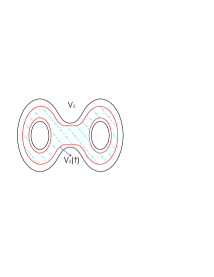
Figure 22: A solid genus-$p$ handle-body contained within $V_{2}$

$$\widetilde{\psi}=\left\{\begin{array}[]{ll}(1-t)I+t\psi&\textrm{on}~{}\partial V_{2}(t)\\ I&\textrm{on}~{}V_{2}(0)\end{array}\right.$$ (14)

Let $X_{2}$ be the vector field corresponding to $\phi_{2}$ on $\partial V_{2}$. Then we ‘twist’ the dynamics on $V_{2}$ by $\psi$, i.e., $(\psi^{-1})_{\ast}X_{2}$ and extend this to $V_{2}$ in an obvious way using (14). Then the dynamics on $\partial V_{2}$ match those on $\partial V_{1}$ according to the Heegaard diagram and the result is proved.   $\Box$

6 Conclusions

In this paper, we have considered a variety of methods for generating systems on 3-manifolds. We have shown how to construct dynamical systems explicitly on hyperbolic 3-manifolds. This is achieved by using a modified theta series to obtain the ‘generalized’ automorphic functions which ‘uniformize’ the vector fields on the manifold. Here we concentrated on using the upper half-space model for the hyperbolic space, while it is also possible to use the disk model. Also we gave an example of how to generate such systems. Also we consider constructing dynamical systems with the help of Reeb foliation. This is achieved by defining a system on each leave and then using the connected sum method to link them together.

In the next paper we shall consider the possible existence of knotted chaotic systems when applying the side-pairing to obtain the 3-manifolds.

References

- [1] Banks, S. P. and Song, Y. “Elliptic and automorphic dynamical systems on surfaces”, Int. J. of Bifurcation and Chaos, Vol. 16, No. 4 (2006) 911-923.
- [2] Candel, A. and Conlon, L. [2000] “Foliations I, II”, Grad. Studies in Maths, AMS.
- [3] Elstrodt, J. [1998] “Groups acting on hyperbolic space: Harmonic analysis and number theory”, Springer-Verlag.
- [4] Ford, L. R. [1929] “Automorphic functions”, McGraw–Hill.
- [5] Hempel, J. [1976] “3-Manifolds”, Ann. Math. Studies, No. 86, Princeton University Press.
- [6] Moerdijk, I. and Mrcun, J. [2003] “Introduction to foliations and Lie groupoids”, Cambridge: CUP.
- [7] Perko, L. [1991] “Differential equations and dynamical systems”, Springer-Verlag, NY.
- [8] Ratcliffe, J. G. [1994] “Foundations of hyperbolic manifolds”, GTM, Vol. 149, Springer-Verlag, NY.