Calorons and dyons at the thermal phase transition
analyzed by overlap fermions
Abstract
In a pilot study, we use the topological charge density defined by the eigenmodes of the overlap Dirac operator (with ultraviolet filtering by mode-truncation) to search for lumps of topological charge in pure gauge theory. Augmenting this search with periodic and antiperiodic temporal boundary conditions for the overlap fermions, we demonstrate that the lumps can be classified either as calorons or as separate caloron constituents (dyons). Inside the topological charge clusters the (smeared) Polyakov loop is found to show the typical profile characteristic for calorons and dyons. This investigation, motivated by recent caloron/dyon model studies, is performed at the deconfinement phase transition for gluodynamics on lattices described by the tadpole improved Lüscher-Weisz action. The transition point has been carefully located. As a necessary condition for the caloron/dyon detection capability, we check that the LW action, in contrast to the Wilson action, generates lattice ensembles, for which the overlap Dirac eigenvalue spectrum smoothly behaves under smearing and under the change of the boundary conditions.
pacs:
11.15.Ha, 11.10.WxI Introduction
The two current confinement scenarios, the monopole ’t Hooft (1975); Mandelstam (1976); ’t Hooft (1981) and the vortex mechanism ’t Hooft (1978); Mack (1980) of confinement in gauge theory have become unified within the vortex picture ’t Hooft (2003); Greensite (2003); ’t Hooft (2004); Di Giacomo (2005); Alkofer and Greensite (2007); Boyko et al. (2006). Yet there exists the old hope to connect confinement also with the topological structure as understood in terms of instantons Fukushima et al. (1997, 1998, 2001), calorons Gerhold et al. (2007), dyons Diakonov (2003); Diakonov and Petrov (2007), merons Lenz et al. (2004) and more generic objects Wagner (2007), all being carriers of Pontryagin charge. 111For brevity, in this paper we understand “calorons”, “dyons” and “selfdual” as including also “anticalorons”, “antidyon” and “antiselfdual”. The main reason for this desire is to bring confinement, on first sight a rather abstract property of pure (lattice) Yang-Mills theory, in closer relation to the physical origin of chiral symmetry breaking and to the continuum theory.
During the last decade new selfdual solutions have entered the discussion. The aim is now to explain confinement in such a model via a detour through finite temperature, at . The new solutions are the Kraan-van Baal-Lee-Lu Kraan and van Baal (1998a, b, c); Lee and Lu (1998) calorons with a general asymptotic holonomy , not necessarily in the center of . For the asymptotic holonomy can be roughly identified with the real-valued spatial average of the Polyakov loop .
Very recently, Diakonov and Petrov have worked out a model Diakonov and Petrov (2007) based on a gas of interacting caloron constituents, i.e. selfdual dyons, that offers already a complete picture of confinement at finite temperature. Although the presence of both selfdual dyons and antiselfdual antidyons has been ignored so far, the model is a convincing step forward. For the success of this description (which describes also the limit of low temperature !) the maximally nontrivial holonomy of the gauge field is crucial.
In one paper Gerhold et al. (2007), authored last year at Humboldt University, the capability of a caloron gas model to explain confinement has been explored in a Monte Carlo study. In this caloron model the opposite extreme case of dyons bound in calorons is dealt with. The importance of maximally nontrivial holonomy for the correct choice of the caloron solutions to be used in the model was the central idea. Even a modest dissociation of calorons into slightly separated dyon-dyon pairs turned out sufficient to create a confining heavy-quark potential of the right order of magnitude.
The assumptions of these models have to be confronted with the lattice. Will we ever have the chance to confirm or disprove models of this type by analyzing generic Monte Carlo lattice configurations ? For some time already our aim is to understand, albeit numerically, to what extent calorons and dyons coexist and are discernible in the Euclidean gauge fields, most probably below . This has been the central question in our two previous lattice papers on the problem Ilgenfritz et al. (2005, 2006) and is the central question also now.
Traditionally, the presence of locally classical excitations like instantons in Monte Carlo lattice gauge fields has been explored by using methods like cooling Teper (1985); Ilgenfritz et al. (1986); Hoek et al. (1987); Polikarpov and Veselov (1988), restricted cooling Garcia Perez et al. (1999), smearing DeGrand et al. (1998a), that replaced the more demanding RG cycling DeGrand et al. (1997); DeGrand et al. (1998b), and more general, by combinations of blocking and inverse blocking DeGrand et al. (1996a, b); Feurstein et al. (1998). In the result, a well-localized topological charge density (according to its field-theoretical definition Di Vecchia et al. (1981, 1982)) becomes visible. All these methods actively change the gluonic field of the lattice configurations. Therefore they have been considered with some scepticism because of the methodical bias towards classical fields. Concerning our particular point of view, one might criticize that these methods also tend to hide the presence of dyonic constituents inside calorons.
For the evaluation of the topological charge density the situation has completely changed with the availability of methods dealing with overlap fermions Neuberger (1998a, b) – or other fermions with improved chiral properties Gattringer (2001); Gattringer et al. (2001) – as a probe to explore gauge fields. A definition Niedermayer (1999); Hasenfratz et al. (1998) of the topological charge density has been given involving the trace of the overlap Dirac operator. Then ultraviolet filtering can be given a well-defined sense Horvath et al. (2003a, b) by restricting the trace to the lowest fermionic eigenmodes with in the spectrum. The properties of this whole family of topological densities are strongly changing with and have been investigated in detail in Ref. Ilgenfritz et al. (2007).
In our two lattice papers Ilgenfritz et al. (2005, 2006) on the caloron/dyon issue we were relying on the smearing technique and using the field-theoretical definition of the topological charge density in terms of an improved lattice field-strength tensor Bilson-Thompson et al. (2003). Additionally, in order to support the interpretation of the clusters of topological charge as calorons or dyons, the monopole content of the clusters has been analyzed in the maximal Abelian gauge. 222MAG was implemented on the lattice first in Refs. Kronfeld et al. (1987); Brandstaeter et al. (1991).
With the present paper we return to the investigation of the caloron/dyon structure. We are replacing the field-theoretical topological charge density, which always requires smearing, by the overlap-based topological charge density in the ultraviolet filtered form mentioned above. We should remind the reader that chirally improved lattice fermions Gattringer (2001); Gattringer et al. (2001) (another realization of Ginsparg-Wilson Ginsparg and Wilson (1982) fermions) have already been used to analyze unsmeared lattice configurations for the presence of calorons Gattringer and Schaefer (2003). Before that, unimproved Wilson fermions have been employed Ilgenfritz et al. (2002) for the description of nearly classical calorons and dyons obtained by cooling. What was common to both techniques was inspired by the theoretically known behavior of zero modes of caloron-like configurations Chernodub et al. (2000). Thus, particular emphasis was first given to the zero modes (or the real modes in case of the Wilson-Dirac operator), which must be present in configurations with topological charge , and to the effect on them of changing the boundary conditions for the Dirac operator Ilgenfritz et al. (2002); Gattringer and Schaefer (2003); Gattringer et al. (2004); Gattringer and Pullirsch (2004). Confronting the zero-mode pattern with the picture revealed by smearing, it became clear Gattringer et al. (2004) that the zero modes are part of the topological structure of a typical Monte Carlo configuration but cannot exhaustively explain it.
In a recent paper Bruckmann et al. (2006) reporting a collaborative project of the Humboldt University and Regensburg University lattice groups, it has been described how smearing and spectral filtering methods (with fermions and scalars) can be tuned to each other as far as the topological charge density is concerned. In our present context the relation between the fermionic filtering and the result of smearing is relevant. In the parameter space of competing methods (number of modes vs. smearing steps) a mapping was defined by optimizing the cross-correlation between the respective topological charge densities. As just two extreme examples we quote the observations that 10 smearing steps are equivalent to the filtering by 50 modes, while 20 smearing steps are equivalent to not more than 8 modes. These are only two arbitrarily taken cases of relatively mild and strong filtering. Of course, the structure changes (the number of lumps decreases) with increasing smearing steps. Moreover, even the parameter mapping does not guarantee that the clusters of the respective densities exactly coincide. The pointwise overlap amounts only to 50 to 60 %. Although in Ref. Bruckmann et al. (2006) chirally improved fermions Gattringer (2001); Gattringer et al. (2001) were employed instead of overlap fermions, the results give additional motivation and orientation for the present investigation and may be helpful to appreciate the new findings. We will explore the possibilities of identifying caloron-like and dyon-like structures for intermediate filtering employing 20 overlap eigenmodes.
What is the conjectured physical picture ? Our previous experience Ilgenfritz et al. (2005, 2006); Gerhold et al. (2007) suggests, in accordance with the model of Diakonov and Petrov Diakonov and Petrov (2007) that a “plasma” including calorons (with nontrivial holonomy) and dissolved dyonic constituents may describe the field structure at rather well. It fails, however, to describe the essential features of lattice fields above . It has been guessed that calorons with intermediate holonomy 333The usual Harrington-Shepard calorons Harrington and Shepard (1978), forming the basis of the first nonperturbative description of finite- QCD Gross et al. (1981), represent the limiting case of trivial holonomy. would describe the topological structure in the high- phase closely above . A semiclassical evaluation of the path integral Diakonov et al. (2004) has shown, however, that the caloron becomes unstable against dissociation into dyons outside a narrow stability region . On the lattice, by suitable measures of selfduality Gattringer (2002); Ilgenfritz et al. (2007), it has been observed that locally selfdual domains become suppressed above . The topological susceptibility is known to slowly decrease (in the case of gauge theory), and purely magnetic monopole excitations probably acquire an overwhelming importance.
In the confined phase the caloron model indeed describes confinement, even if the dissociation of calorons into dyons remains incomplete and within a description by a phenomenological choice of the distribution. The size variable in the caloron case represents a natural extension of the size parameter , usually assigned to the (Euclidean) spherical lumps of action seen at , to higher temperatures in the confinement phase when the distance between the constituents may be or bigger. Dissociation is increasing with rising temperature towards . 444This tendency is also supported by the cooling results in Ref. Ilgenfritz et al. (2004). This is in agreement with a practically temperature independent -distribution for , similar to the usual instanton parametrization Gerhold et al. (2007). Let us remark that at very low temperature the carriers of topological charge become more and more difficult to distinguish from genuine instantons by means of gauge-invariant observables alone (action and topological charge density). All this has lead to the conjecture that close to the deconfining phase transition the dyonic content of calorons becomes maximally manifest. Therefore we concentrate here first on this temperature.
In the present investigation we have dispensed with (i) the use of smearing for the detection of clusters of topological charge, and with (ii) the maximally Abelian gauge needed to determine the monopole content of the latter. We gave up, on the other hand, the exclusive focus on the zero mode(s) Gattringer and Schaefer (2003); Gattringer and Pullirsch (2004) of the configurations being under investigation. We have concentrated instead on the effect of changing the fermionic boundary conditions on the whole overlap-based topological charge density mapped out by a given (not too large) number of eigenmodes. The dependence on boundary conditions has not yet been systematically investigated. Our present paper is a first step in this direction and hopefully stimulates such a thorough investigation. Also concerning the gauge theory, this paper is the first application of the overlap-based topological charge density. For two colors it suffices to restrict oneself to the simultaneous consideration of periodic vs. antiperiodic boundary conditions. We shall see that the mode-truncated topological charge densities corresponding to the two boundary conditions, completed by the local Polyakov loop, allow us to classify the visible topological charge clusters as calorons and separate dyons, respectively.
The paper is organized as follows. In section II we define the technical details of our analysis: the action Lüscher and Weisz (1985); Curci et al. (1983), the overlap Dirac operator Neuberger (1998a, b) and the corresponding topological charge density Niedermayer (1999); Hasenfratz et al. (1998). Under conditions of confinement, but close to the transition temperature, we critically check the stability of the fermionic topological charge (given by the index of the overlap Dirac operator) and the continuity of the low-lying spectrum under smearing and with respect to a change of fermionic boundary conditions. This check forces us to abandon the standard Wilson gauge action and motivates the choice of the Lüscher-Weisz action that successfully passes the test. The bulk of investigations is performed using the tadpole-improved Lüscher-Weisz action Gattringer et al. (2002). In section III we determine the critical for the quenched thermal phase transition with this action. The search for the transition is restricted to a lattice that will be used in the following. Next, in section IV, we explain how the mode-truncated, overlap-based topological charge density obtained with the two different fermionic boundary conditions can be used to extract calorons and dyons from unsmeared configurations, but restricted to the resolution given by the number of eigenmodes. This is practised for an ensemble generated on top of the phase transition. In the future we hope to proceed with this analysis deeper into the confinement and the deconfinement phases. A discussion of the results in the light of related work, our conclusions and an outlook will be presented in section V.
II Wilson vs. Lüscher-Weisz action: the stability of the Dirac spectrum
II.1 The action
We employ for the actual analysis of the caloron/dyon content of gauge theory the tadpole improved action of the Lüscher-Weisz form Alford et al. (1995); Bornyakov et al. (2005)
| (1) |
where and denote plaquette and rectangular loop terms in the action,
| (2) |
The parameter is the input tadpole improvement factor taken here equal to the fourth root of the average plaquette . For gauge theory, the tadpole factor has been selfconsistently determined first in Ref. Bornyakov et al. (2005) for a few values in the case of vanishing temperature on lattices with a suitable lattice size for each value of the bare coupling constant. The result is given in Table I. For the convenience of the reader and later reference to the lattice scales we present the corresponding values of the string tension in lattice units.
| L | ||||
|---|---|---|---|---|
| 2.7 | 12 | 0.87164 | 0.87165(2) | 0.60(5) |
| 3.0 | 12 | 0.89485 | 0.89478(2) | 0.366(8) |
| 3.1 | 12 | 0.90069 | 0.90069(1) | 0.309(6) |
| 3.2 | 16 | 0.90578 | 0.905765(3) | 0.258(5) |
| 3.3 | 16 | 0.91015 | 0.910152(4) | 0.219(3) |
| 3.4 | 20 | 0.91402 | 0.914020(2) | 0.180(3) |
| 3.5 | 20 | 0.91747 | 0.917481(1) | 0.151(3) |
In our simulations we have not included one-loop corrections to the coefficients nor considered non-planar 6-link loops the coefficient of which would be purely perturbative. We have adopted the values obtained at zero temperature also for the simulations at .
II.2 The overlap Dirac operator
The overlap Dirac operator is a particular solution of the Ginsparg-Wilson relation Ginsparg and Wilson (1982)
| (3) |
where is a dimensionless parameter not to be confused 555We prefer to keep this standard notation. with the instanton or caloron size parameter above. These operators have nearly perfect chiral properties. In particular, the Atiyah-Singer index theorem is fulfilled at finite lattice spacing, with clearly recognizable zero modes with positive or negative chirality related to the topological charge
| (4) |
This is unambiguous as long as the configurations satisfy certain weak smoothness requirements Hernandez et al. (1999). A Neuberger operator can be constructed starting from an arbitrary input Dirac operator (with bad chiral symmetry or with already improved chiral symmetry) through the steps we describe now. In our case, we take as the input kernel the simple Wilson-Dirac operator. In this case, the emerging Neuberger overlap operator Neuberger (1998a, b) is
| (5) |
where is the Wilson-Dirac operator with a negative mass term . is the Wilson hopping term with . An optimal choice is . By construction, the operator satisfies the Ginsparg-Wilson relation. In order to compute the sign function in the alternative expression
| (6) |
we have used the minmax polynomial approximation Giusti et al. (2003). Furthermore, the low-mode projection has been used: 80 eigenmodes of the hermitean Wilson-Dirac operator have been treated explicitely.
The topological charge density can be expressed in the form Niedermayer (1999)
| (7) |
where denotes the trace only over color and spinor indices. This form of the topological charge density contains vacuum fluctuations of all scales. In the apparent chaos remarkable global, low-dimensional structures Horvath et al. (2002, 2003c); Horvath (2005) are formed. They are three-dimensional at the percolation threshold Ilgenfritz et al. (2007). The ultraviolet filtered (mode-truncated) density Horvath et al. (2003a) is written as a truncated sum over as the dimensionless eigenvalues of ,
| (8) |
however, shows clustering of topological charge Ilgenfritz et al. (2007) in four-dimensionally coherent clusters similar Bruckmann et al. (2006) to structures usually revealed by smoothing the gauge field. This is the level of resolution where calorons and dyons may appear (or not).
The integral over gives corresponding to the Atiyah-Singer index theorem, independent of , because only the zero modes contribute to according to their chirality. It is remarkable, but generally observed for the overlap Dirac operator, that if there are zero modes within a configuration, they all have the same chirality.
II.3 The Dirac spectrum under smearing and varying boundary conditions
The cross-relation between topological charge density and local structure of the Polyakov loop is typical for calorons and their constituents. In order to map out the Polyakov loop we need a modest amount of APE smearing in this study. A second role of smearing in our present context is that we want to monitor the independence of the index of the overlap Dirac operator and a smooth dependence of the low lying spectrum on the number of APE smearing steps. We regard this as a necessary prerequisite that this part of the spectrum reflects medium-scale and infrared properties only. Thus, a minimal requirement for the Dirac operator as well as for the lattice action (to prevent lattice artefacts that could give rise to unphysical zero modes) is the continuity of the spectrum under moderate smearing. This in fact selects admissible actions and an admissible range of the respective coupling.
Smearing is an iterative sequence of four-dimensional link substitutions, where links are replaced by a weighted average of the links and the staples
surrounding it:
| (9) |
Here denotes the projection onto the gauge group. For this is just a rescaling of the matrix by a scalar. We choose the smearing parameter following DeGrand et al. (1998a) where an optimal smearing schedule has been searched for. Within some limits, this parameter could be traded against the number of smearing steps. We allow for iterations.
(a)
(b)
It is known since long Göckeler et al. (1989) that the Wilson action is problematic with respect to dislocations. We remind the reader that the definition of a dislocation depends both on the action in use for the generation of gauge configurations and on the prescription chosen to define the topological charge (or charge density). In the case of the Wilson action together with the (geometrical) Phillips-Stone topological charge Phillips and Stone (1986), scaling of the topological susceptibility Kremer et al. (1988) was an unsuspected fact before Pugh and Teper Pugh and Teper (1989a) have shown that the observed value of was dominated by excitations of size that would not survive blocking. The lesson we draw from this example is that the bosonic topological charge
| (10) |
to be assigned to a configuration by a suitably improved gluonic topological charge density
| (11) |
and a geometrically defined version of the topological charge Phillips and Stone (1986); Lüscher (1982) may be in systematical disagreement due to the presence of lattice artefacts. This can be the case even though it might not appear as a scaling violation of the topological susceptibility. In a first application of the overlap operator to gauge fields generated with Wilson action Gubarev et al. (2005), a reasonable continuum limit of the susceptibility with defined via the index of the overlap operator has been found. Therefore the Wilson action was not suspicious. The value of , however, was somewhat large compared to other estimates for the gauge theory. 666The scaling property of the topological susceptibility would only be lost, resulting in a diverging susceptibility in the continuum limit, if local excitations would exist, that give rise to highly localized zero modes and would have a Wilson action less than Pugh and Teper (1989b).
The field-theoretic definition of the topological charge density that we have used in our previous papers Ilgenfritz et al. (2005, 2006) employs the improved field strength tensor Bilson-Thompson et al. (2003). The geometrical definition of the topological charge of a configuration is replaced in our present context by the index of the overlap Dirac operator, and the topological density by the corresponding expression (7) given above. At this point, checking the above-formulated requirements, disturbing features of the Wilson action are encountered. At first, the roughness of the configurations results in a relatively bad performance of the ARPACK package used to diagonalize the overlap Dirac operator. This probably leads to a bad reproducibility of the measured index. Thus, the latter can easily be misidentified due to zero modes pinned to dislocations. During the first smearing steps such dislocations become even more singular.
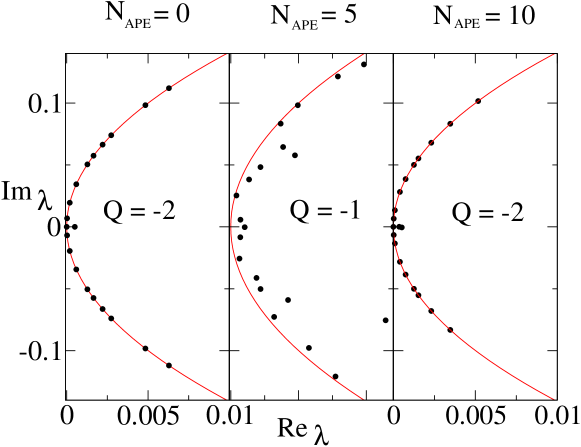
As a typical example we show in Fig. 1 the lowest 20 eigenvalues according to the two boundary conditions imposed, without smearing and with 5 and 10 smearing steps, for a configuration generated with the Wilson action at . This was chosen below the critical value reported for the Wilson action in Ref. Fingberg et al. (1993). We see jumps of the measured topological charge, , between subsequent stages of smearing and occurring under a change of the boundary conditions (temporally periodic vs. antiperiodic). During the first steps, smearing changes only the short range structure. The changing index counts here essentially the dislocations. Hence, the number of zero modes rapidly changes with the APE smearing steps.
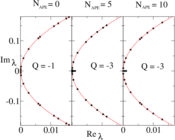
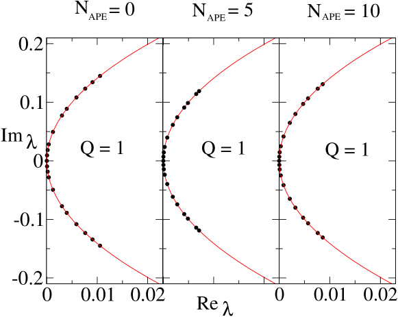
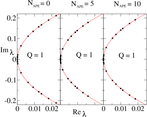
The fact that the Lüscher-Weisz action is advantageous to facilitate our study, has been confirmed for a number of values. The result is demonstrated in Fig. 2 for a typical configuration from a Lüscher-Weisz ensemble at . The number of zero modes is independent of the type of temporal boundary condition and does not change with the number of APE smearing steps (as long as smearing is moderate, say ). For we have never encountered such ambiguities as seen in the Wilson case. In Section III we will see that the critical inverse gauge coupling for this action is . The successful check presented in Fig. 2 has been performed for a situation close but clearly below the phase transition.
We should stress, however, that configurations created by means of the Lüscher-Weisz action may also turn out too “rough” at sufficiently low values. For example, exploring the temperature range around on a coarser lattice with (i.e. at lower ), we found that the described ambiguities reappear.
A surprising observation in the case of both actions is that the interval covered by the 20 lowest eigenvalues does not systematically expand under the application of smearing steps. This differs from the behavior seen in Ref. Gattringer et al. (2006) for configurations generated with the (tree-level) Lüscher-Weisz action. The spectrum there was considered not for the overlap Dirac operator but for the chirally improved Dirac operator proposed in Ref. Gattringer (2001); Gattringer et al. (2001). It would be interesting to compare the two Dirac operators in their behavior under smearing for different lattice ensembles (provided the smearing-induced changes are smooth).
(a)
(b)
III Locating the finite temperature phase transition
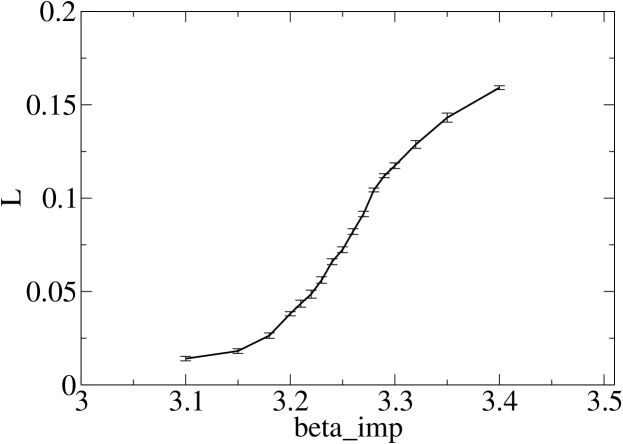
The last observations make clear that we need to choose for the purpose of this investigation. Let us now look for a more precise location of the deconfinement transition. On the lattice, varying , we have studied the behavior of the Polyakov loop and of the Polyakov loop susceptibility. We used a polynomial fit for as a function of , based on the measured values shown in Table I, in order to provide the corresponding tadpole improvement factor for each simulation point . We stress again that this non-perturbative determination, strictly speaking, is well-established only for temperature .
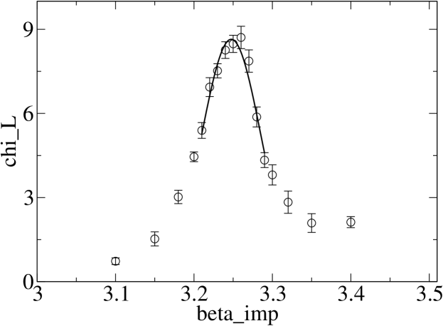
We have measured the Polyakov loop and its susceptibility in the range from to with different statistics per data point. The simulation data between and 3.29, in the immediate vicinity of the phase transition, have been collected in 100,000 to 300,000 Monte Carlo sweeps per value while the Polyakov loop was measured after every sweep. In the closer vicinity of the phase transition we have fitted the susceptibility data by a Gaussian. The data and the fit of the susceptibility are presented in Fig. 3. For the determination of the errors, the blocked jackknife method was used with a block size of 2000 measurements. From the fit we are able to locate the deconfinement transition at for . This confirms our preliminary choice made in Sect. II of for a check of smoothness of the overlap Dirac operator that should be done in the confinement phase on a lattice of the same size. Interpolating the data in Table I we estimate at corresponding to .
(a)
(b)
IV Finding calorons and dyons using periodic and antiperiodic modes
In the Introduction we have argued why we should first search on top of the phase transition for calorons with nontrivial holonomy and why we anticipate to find them partly separated into dyons. We have chosen very close to the transition point for the following study of topological charge clustering. Our analysis is based on lowest-lying modes for an ensemble of quenched configurations at the deconfinement transition. This was a realistic task within the capability of a standard modern PC within a few weeks.
The topological charge density of an equilibrium Monte Carlo field configuration is represented by the mode-truncated, i.e. ultraviolet filtered, topological charge density (8). In that definition the temporal boundary condition was not specified, that should be applied in the construction of the Wilson-Dirac and the Neuberger overlap operator (5). From the work of Gattringer and Schaefer Gattringer and Schaefer (2003) we know that the single zero mode of a Monte Carlo configuration eventually hops between positions. On the other hand, the topological charge density of a (quenched) lattice configuration cannot depend on the purely analysing fermions, in particular not on the boundary conditions imposed to them. The most suggestive rule for the topological charge density, if given by the zero-mode part of (8) alone, would be to average over the boundary conditions, which eventually (but not always !) lead to a different localization of the zero mode. This recipe is now applied to the topological charge density with the inclusion of the low-lying non-zero modes, too.
(a)
(b)
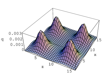
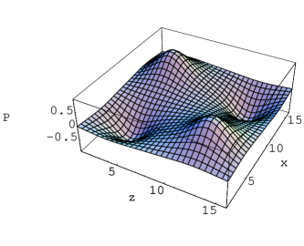
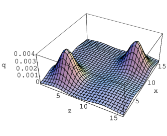
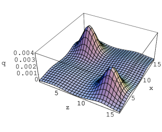
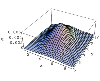
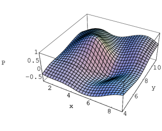
We illustrate this in Fig. 4 for a classical charge caloron solution with nontrivial holonomy in a state of maximal separation into four dyons. The upper panels show the gluonic definition of the topological charge density and the profile of the Polyakov loop over a two-dimensional section of a lattice. The gluonic topological charge density recognizes all the four constituents as positive peaks while the Polyakov loop distinguishes the constituents according to the local holonomy, i.e. positive and negative values of the Polyakov loop. In the fermionic definition of the topological charge density, , we content ourselves to only 20 lowest modes. We find that this filtered density depends on the boundary condition , with denoting periodic and denoting antiperiodic temporal boundary conditions. The charge densities present a different profile depending on the type of boundary conditions. The antiperiodic boundary condition highlights the constituents with negative local Polyakov loop, whereas the periodic boundary condition emphasizes the complementary constituents with positive local Polyakov loop. The “true” topological charge density (that is well-represented by the gluonic definition in this classical case) is well approximated by an average of the two fermionic topological charge density functions and ,
| (12) |
where the superscript or of the modes (the subscript of the eigenvalues) refers to the boundary condition.
(a)
(b)
Thus, for each boundary condition, we will search for peaks of the modulus of the corresponding fermionic topological charge density. In addition, in order to define a size for the charge cloud surrounding the peaks, the respective topological charge density is separately subjected to a cluster analysis. As usual (see Ref. Ilgenfritz et al. (2005, 2006, 2007)) the cluster analysis is a procedure to identify connected clusters among those lattice sites , that have been selected by the condition that the modulus of the topological charge density exceeds a certain threshold value . Two sites , being neighbors on the lattice, belong to the same cluster, if the signs of and agree. Otherwise they belong to different clusters. Guided by Ref. Bruckmann et al. (2006), the threshold is chosen relative to the maximal density in the configuration as , safely above the point where the clusters coalesce and, finally, percolate.
(a)
(b)
For the set () of clusters in a configuration found by the cluster analysis of the two densities and , respectively 777For convenience we simplify the notation from now by dropping the subscript from ., we record the maximal value of the modulus of the corresponding density,
| (13) |
the sign and the corresponding space-time position of the peak inside each cluster . The main purpose of defining the finite size clusters around the peaks is to characterize the behavior of the Polyakov loop in the vicinity. The Polyakov loop is always measured after smearing steps. Although the sign of the Polyakov loop at the cluster centers (topological density peaks) is found to be dictated by the temporal periodicity/antiperiodicity imposed on the Dirac operator, the Polyakov loop is monitored all over the cluster to give auxiliary information. Its extremal values, and , inside the clusters are recorded. At least one of the two corresponds to the fermionic boundary condition that defines the clusters, being positive for the periodic boundary condition and negative for the antiperiodic boundary condition.
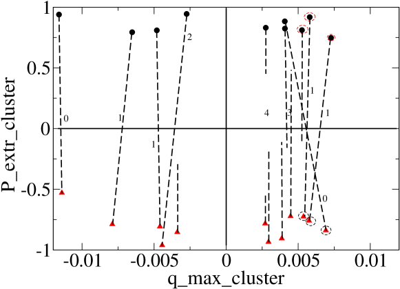
Figs. 5 (a) and (b) show “cluster plots” representing two typical lattice configurations. A cluster of the topological charge density is represented in the cluster plot by a filled circle () for the periodic boundary condition or by a filled triangle () for the antiperiodic boundary condition. The clusters are plotted in Figs. 5 at the appropriate position
| (14) |
in the plane. Here denotes either or , according to the or boundary condition that has defined the cluster through the corresponding topological charge density. Notice that this means that all circles appear in the upper and all triangles in the lower half-plane.
Sometimes it happens that after changing the boundary condition from periodic to antiperiodic, one of the new clusters, , nearly coincides in its space-time position with one of the previous ones, , with a shift of the peak position less than a distance in space-time. This would correspond to the “not jumping” case of Ref. Gattringer and Schaefer (2003) where, however, only the scalar density of a single zero mode was under consideration. In this case, such clusters, the circle and the triangle , are connected in Fig. 5 by a broken line. The numbers close to the lines denote the approximate shift (0 or 1 or 2) of the peak position. Such a pair represents a complete “caloron”, and the average over the respective topological charge densities and locally represents the true topological charge density inside the caloron. For calorons the topological charge clusters defined for both types of boundary conditions are such that inside the clusters the extremal values of the Polyakov loop, and , have clearly an opposite sign, indicative for the dipole structure of a caloron in terms of the Polyakov loop.
Clusters that remained unpaired in this “cluster plot” have appeared only once, under only one type of boundary condition, such that the peak position could not be identified with a peak of the opposite boundary condition, within a tolerance . This corresponds to the “jumping” case of Ref. Gattringer and Schaefer (2003). Such clusters do not have an obvious partner (with opposite sign Polyakov loop and same sign topological charge density) suitable to form a “caloron”. The length of the broken line attached to the unpaired filled symbols represents the difference between the maximum and the minimum of the Polyakov loop inside the cluster. Numbers close to the unconnected lines denote the approximate distance (in the example, 3 or 4) between the cluster centers. In contrast to the caloron clusters both maximum and minimum of the Polyakov loop in an unpaired cluster are mostly of the same sign. In the few remaining cases the wrong-sign extremum is close to zero. Such clusters are called “dyons” because they, like the dyons in the classical caloron solution shown in Fig. 4, are invisible to the fermions under the “wrong” boundary condition.
The open circles around the filled symbols in the plots emphasize clusters which would have been localized knowing the zero mode(s) alone. These can also be clusters that we have to classify as calorons and as dyons. If they exist in the same configuration, these are clusters of a unique sign of the topological density, in accordance to the (yet unexplained) empirical fact that all zero modes of one configuration have the same sign of chirality. 888The cases of more than one zero mode per configuration were excluded from the analysis in Ref. Gattringer and Schaefer (2003).
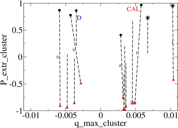
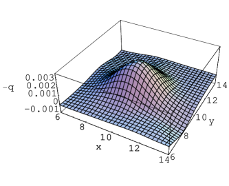
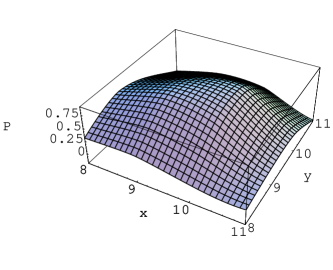
Two characteristic objects that have been marked in Fig. 5 (b) as “CAL” and “D” are visualized in Fig. 6 in magnified form by their fermionic topological charge density profile (left) and their Polyakov loop profile (right) within the occupied part of an - section: (a) for the caloron possessing the characteristic dipole structure of the Polyakov loop and (b) for the dyon possessing a broad maximum of the Polyakov loop. Let us stress that these objects have been identified in a generic Monte Carlo lattice configuration without cooling or smearing. To be sure, the Polyakov loop is presented after 10 smearing steps, which explains the smooth picture.
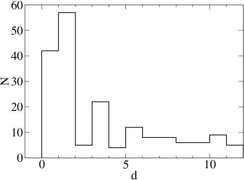
We have also studied the relative separation of appropriate dyon pairs. In Fig. 7 an histogram of dyon-dyon distances in our sample is presented. The first two bins correspond to calorons with distances . The rest of the histogram with contains pairs of suitably fitting dyon-dyon pairs, i.e. with the same sign of and an opposite sign of , grouped into pairs according to the closest distance. The statistics does not warrant so far the comparison with a specific model for the caloron/dyon plasma.
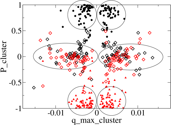
Finally, we have collected in Fig. 8 all clusters of the whole sample of 20 configurations analogously to Fig. 5. The unpaired dyons are placed at their original positions in the plane. The difference to Fig. 5 is that the two clusters close in space-time corresponding to an undissociated caloron in this plot are re-located according to the average of the Polyakov loop assigned to the respective cluster as follows,
| (15) |
a value which is scattered around zero because of the dipole structure. Thus, in Fig. 8, each undissociated caloron is still represented by a close pair (with and ) of open squares, now with . The re-location according to the averaged Polyakov loop following Eq. (15) leads in this scatter plot of clusters to a separation of points representing calorons and anticalorons (clustered in the ellipses) from the four types of dyons (clustered in the four circles) with .
The total number of isolated dyons (separated by a distance ) is 113 plus 126 in this ensemble, whereas the number of dyons confined inside calorons (with a distance ) amounts to 101 plus 101, meaning that on average approximately 10 calorons (dissociated or not) are present per configuration, if the resolution corresponds to 20 overlap eigenmodes. We emphasize again that the counting is a counting of peaks. All peaks get classified as dyons, regardless whether isolated or confined in calorons. The total number corresponds to a caloron (or dyon pair) density . This in the right ballpark set by the topological susceptibility, given the relative arbitrariness of the number of filtering modes.
V Conclusion
In this paper we have continued our search for specific KvB caloron-like features in finite- lattice configurations. In a feasibility study we have for the first time employed overlap valence fermions for this diagnostic purpose. More specifically, we have employed the dependence of eigenvectors and eigenvalues on the temporal boundary conditions imposed on the Dirac operator that can be changed at will. Thereby, we have taken into consideration not only the zero mode(s) but the UV filtered topological charge density restricted to the 20 lowest modes per configuration. The dependence of the apparent caloron/dyon content on the number of eigenmodes has still to be systematically looked for. According to Ref. Bruckmann et al. (2006) a resolution provided by 20 lowest fermionic eigenmodes, roughly corresponds to an amount of smoothing between 10 and 20 smearing steps.
In our previous work Ilgenfritz et al. (2005, 2006) we have used smearing and the corresponding gluonic topological density. The amount of smearing was, also somewhat arbitrarily, defined by the requirement that the string tension should not drop below 60 % of the full string tension Ilgenfritz et al. (2006) which allowed for 50 or 25 … 20 smearing steps in the confinement or deconfinement phase, respectively. Even more arbitrarily, the threshold for the definition of the clusters was set such that the density is split into a maximal number of clusters. Under these circumstances, a large number of shallow clusters entered the investigation before only a small part of the clusters could be successfully characterized – by the monopole content – as calorons or dyons.
In this work, apart from the number of modes dictated by the PC memory, we have fixed the cutoff in a region where the number of clusters does not change with the cutoff and the size changes slowly. Moreover, the cluster centers were localized by the peaks of the modulus of the fermionic topological density and do not change anymore with the cutoff. Thus, the number of clusters is determined essentially by the number of analysing modes that was adopted in anticipation of a physically acceptable density of dyon pairs. What we could show here is that with this resolution the cluster composition of the topological charge can be understood in terms of calorons and dyons without serious problems.
All these clusters, once found, are seen to be accompanied either by a dipole structure in the Polyakov loop or a broad maximum of the modulus of the Polyakov loop . This shows that by means of the two topological densities (corresponding to periodic or antiperiodic temporal boundary conditions for overlap fermions) the task can be solved to identify calorons and dyonic constituents.
In future investigations we will have to further specify those conditions for filtering that make the cluster charges distributed around and , hopefully a very stable result. Furthermore, we hope for a better confirmation of the caloron/dyon model by extending this study to lower temperature (where the model is good for describing confinement) and to study also the higher temperature region.
Acknowledgements
This work was partly supported by RFBR grants 05-02-16306, 06-02-04014 and 06-02-16309 and by the DFG grant 436 RUS 113/739/0-2 together with the RFBR-DFG grant 06-02-04010. Three of us (V.G. B, B.V. M. and A.I. V.) gratefully appreciate the support of Humboldt-University Berlin where this work was carried out to a large extent. S.M. M. is also supported by an INTAS YS fellowship 05-109-4821. E.-M. I. is supported by DFG (FOR 465 / Mu932/2).
References
- ’t Hooft (1975) G. ’t Hooft, Proceedings of the EPS International Conference, Palermo 1975, ed. A. Zichichi, Editrice Compositori, Bologna 1976 (1975).
- Mandelstam (1976) S. Mandelstam, Phys. Rept. 23, 245 (1976).
- ’t Hooft (1981) G. ’t Hooft, Nucl. Phys. B190, 455 (1981).
- ’t Hooft (1978) G. ’t Hooft, Nucl. Phys. B138, 1 (1978).
- Mack (1980) G. Mack, Recent Developments in Gauge Theories, ed. by G. ’t Hooft et al. (Plenum, New York, 1980 (1980), report DESY 80/03.
- ’t Hooft (2003) G. ’t Hooft, Nucl. Phys. A721, 3 (2003).
- Greensite (2003) J. Greensite, Prog. Part. Nucl. Phys. 51, 1 (2003), eprint hep-lat/0301023.
- ’t Hooft (2004) G. ’t Hooft (2004), eprint hep-th/0408183.
- Di Giacomo (2005) A. Di Giacomo, Acta Phys. Polon. B36, 3723 (2005), eprint hep-lat/0510065.
- Alkofer and Greensite (2007) R. Alkofer and J. Greensite, J. Phys. G34, S3 (2007), eprint hep-ph/0610365.
- Boyko et al. (2006) P. Y. Boyko et al., Nucl. Phys. B756, 71 (2006), eprint hep-lat/0607003.
- Fukushima et al. (1997) M. Fukushima et al., Phys. Lett. B399, 141 (1997), eprint hep-lat/9608084.
- Fukushima et al. (1998) M. Fukushima, H. Suganuma, A. Tanaka, H. Toki, and S. Sasaki, Nucl. Phys. Proc. Suppl. 63, 513 (1998), eprint hep-lat/9709133.
- Fukushima et al. (2001) M. Fukushima, E.-M. Ilgenfritz, and H. Toki, Phys. Rev. D64, 034503 (2001), eprint hep-ph/0012358.
- Gerhold et al. (2007) P. Gerhold, E.-M. Ilgenfritz, and M. Müller-Preussker, Nucl. Phys. B760, 1 (2007), eprint hep-ph/0607315.
- Diakonov (2003) D. Diakonov, Prog. Part. Nucl. Phys. 51, 173 (2003), eprint hep-ph/0212026.
- Diakonov and Petrov (2007) D. Diakonov and V. Petrov (2007), eprint arXiv:0704.3181 [hep-th].
- Lenz et al. (2004) F. Lenz, J. W. Negele, and M. Thies, Phys. Rev. D69, 074009 (2004), eprint hep-th/0306105.
- Wagner (2007) M. Wagner, Phys. Rev. D75, 016004 (2007), eprint hep-ph/0608090.
- Kraan and van Baal (1998a) T. C. Kraan and P. van Baal, Phys. Lett. B428, 268 (1998a), eprint hep-th/9802049.
- Kraan and van Baal (1998b) T. C. Kraan and P. van Baal, Nucl. Phys. B533, 627 (1998b), eprint hep-th/9805168.
- Kraan and van Baal (1998c) T. C. Kraan and P. van Baal, Phys. Lett. B435, 389 (1998c), eprint hep-th/9806034.
- Lee and Lu (1998) K.-M. Lee and C.-H. Lu, Phys. Rev. D58, 025011 (1998), eprint hep-th/9802108.
- Ilgenfritz et al. (2005) E.-M. Ilgenfritz, B. V. Martemyanov, M. Müller-Preussker, and A. I. Veselov, Phys. Rev. D71, 034505 (2005), eprint hep-lat/0412028.
- Ilgenfritz et al. (2006) E.-M. Ilgenfritz, B. V. Martemyanov, M. Müller-Preussker, and A. I. Veselov, Phys. Rev. D73, 094509 (2006), eprint hep-lat/0602002.
- Teper (1985) M. Teper, Phys. Lett. B162, 357 (1985).
- Ilgenfritz et al. (1986) E.-M. Ilgenfritz, M. L. Laursen, G. Schierholz, M. Müller-Preussker, and H. Schiller, Nucl. Phys. B268, 693 (1986).
- Hoek et al. (1987) J. Hoek, M. Teper, and J. Waterhouse, Nucl. Phys. B288, 589 (1987).
- Polikarpov and Veselov (1988) M. I. Polikarpov and A. I. Veselov, Nucl. Phys. B297, 34 (1988).
- Garcia Perez et al. (1999) M. Garcia Perez, O. Philipsen, and I.-O. Stamatescu, Nucl. Phys. B551, 293 (1999), eprint hep-lat/9812006.
- DeGrand et al. (1998a) T. A. DeGrand, A. Hasenfratz, and T. G. Kovacs, Nucl. Phys. B520, 301 (1998a), eprint hep-lat/9711032.
- DeGrand et al. (1997) T. A. DeGrand, A. Hasenfratz, and T. G. Kovacs, Nucl. Phys. B505, 417 (1997), eprint hep-lat/9705009.
- DeGrand et al. (1998b) T. A. DeGrand, A. Hasenfratz, and T. Kovacs, Prog. Theor. Phys. Suppl. 131, 573 (1998b), eprint hep-lat/9801037.
- DeGrand et al. (1996a) T. A. DeGrand, A. Hasenfratz, and D.-c. Zhu, Nucl. Phys. B475, 321 (1996a), eprint hep-lat/9603015.
- DeGrand et al. (1996b) T. A. DeGrand, A. Hasenfratz, and D.-c. Zhu, Nucl. Phys. B478, 349 (1996b), eprint hep-lat/9604018.
- Feurstein et al. (1998) M. Feurstein, E.-M. Ilgenfritz, M. Müller-Preussker, and S. Thurner, Nucl. Phys. B511, 421 (1998), eprint hep-lat/9611024.
- Di Vecchia et al. (1981) P. Di Vecchia, K. Fabricius, G. C. Rossi, and G. Veneziano, Nucl. Phys. B192, 392 (1981).
- Di Vecchia et al. (1982) P. Di Vecchia, K. Fabricius, G. C. Rossi, and G. Veneziano, Phys. Lett. B108, 323 (1982).
- Neuberger (1998a) H. Neuberger, Phys. Lett. B417, 141 (1998a), eprint hep-lat/9707022.
- Neuberger (1998b) H. Neuberger, Phys. Lett. B427, 353 (1998b), eprint hep-lat/9801031.
- Gattringer (2001) C. Gattringer, Phys. Rev. D63, 114501 (2001), eprint hep-lat/0003005.
- Gattringer et al. (2001) C. Gattringer, I. Hip, and C. B. Lang, Nucl. Phys. B597, 451 (2001), eprint hep-lat/0007042.
- Niedermayer (1999) F. Niedermayer, Nucl. Phys. Proc. Suppl. 73, 105 (1999), eprint hep-lat/9810026.
- Hasenfratz et al. (1998) P. Hasenfratz, V. Laliena, and F. Niedermayer, Phys. Lett. B427, 125 (1998), eprint hep-lat/9801021.
- Horvath et al. (2003a) I. Horvath et al., Phys. Rev. D67, 011501 (2003a), eprint hep-lat/0203027.
- Horvath et al. (2003b) I. Horvath et al., Nucl. Phys. Proc. Suppl. 119, 688 (2003b), eprint hep-lat/0208031.
- Ilgenfritz et al. (2007) E.-M. Ilgenfritz et al. (2007), eprint arXiv:0705.0018 [hep-lat].
- Bilson-Thompson et al. (2003) S. O. Bilson-Thompson, D. B. Leinweber, and A. G. Williams, Ann. Phys. 304, 1 (2003), eprint hep-lat/0203008.
- Kronfeld et al. (1987) A. S. Kronfeld, G. Schierholz, and U. J. Wiese, Nucl. Phys. B293, 461 (1987).
- Brandstaeter et al. (1991) F. Brandstaeter, U. J. Wiese, and G. Schierholz, Phys. Lett. B272, 319 (1991).
- Ginsparg and Wilson (1982) P. H. Ginsparg and K. G. Wilson, Phys. Rev. D25, 2649 (1982).
- Gattringer and Schaefer (2003) C. Gattringer and S. Schaefer, Nucl. Phys. B654, 30 (2003), eprint hep-lat/0212029.
- Ilgenfritz et al. (2002) E.-M. Ilgenfritz, B. V. Martemyanov, M. Müller-Preussker, S. Shcheredin, and A. I. Veselov, Phys. Rev. D66, 074503 (2002).
- Chernodub et al. (2000) M. N. Chernodub, T. C. Kraan, and P. van Baal, Nucl. Phys. Proc. Suppl. 83, 556 (2000), eprint hep-lat/9907001.
- Gattringer et al. (2004) C. Gattringer et al., Nucl. Phys. Proc. Suppl. 129, 653 (2004), eprint hep-lat/0309106.
- Gattringer and Pullirsch (2004) C. Gattringer and R. Pullirsch, Phys. Rev. D69, 094510 (2004), eprint hep-lat/0402008.
- Bruckmann et al. (2006) F. Bruckmann et al. (2006), eprint hep-lat/0612024.
- Harrington and Shepard (1978) B. J. Harrington and H. K. Shepard, Phys. Rev. D17, 2122 (1978).
- Gross et al. (1981) D. J. Gross, R. D. Pisarski, and L. G. Yaffe, Rev. Mod. Phys. 53, 43 (1981).
- Diakonov et al. (2004) D. Diakonov, N. Gromov, V. Petrov, and S. Slizovskiy, Phys. Rev. D70, 036003 (2004), eprint hep-th/0404042.
- Gattringer (2002) C. Gattringer, Phys. Rev. Lett. 88, 221601 (2002), eprint hep-lat/0202002.
- Ilgenfritz et al. (2004) E.-M. Ilgenfritz, B. V. Martemyanov, M. Müller-Preussker, and A. I. Veselov, Phys. Rev. D69, 114505 (2004), eprint hep-lat/0402010.
- Lüscher and Weisz (1985) M. Lüscher and P. Weisz, Commun. Math. Phys. 97, 59 (1985).
- Curci et al. (1983) G. Curci, P. Menotti, and G. Paffuti, Phys. Lett. B130, 205 (1983).
- Gattringer et al. (2002) C. Gattringer, R. Hoffmann, and S. Schaefer, Phys. Rev. D65, 094503 (2002), eprint hep-lat/0112024.
- Alford et al. (1995) M. G. Alford, W. Dimm, G. P. Lepage, G. Hockney, and P. B. Mackenzie, Phys. Lett. B361, 87 (1995), eprint hep-lat/9507010.
- Bornyakov et al. (2005) V. G. Bornyakov, E.-M. Ilgenfritz, and M. Müller-Preussker, Phys. Rev. D72, 054511 (2005), eprint hep-lat/0507021.
- Hernandez et al. (1999) P. Hernandez, K. Jansen, and M. Lüscher, Nucl. Phys. B552, 363 (1999), eprint hep-lat/9808010.
- Giusti et al. (2003) L. Giusti, C. Hoelbling, M. Lüscher, and H. Wittig, Comput. Phys. Commun. 153, 31 (2003), eprint hep-lat/0212012.
- Horvath et al. (2002) I. Horvath et al. (2002), eprint hep-lat/0212013.
- Horvath et al. (2003c) I. Horvath et al., Phys. Rev. D68, 114505 (2003c), eprint hep-lat/0302009.
- Horvath (2005) I. Horvath, Nucl. Phys. B710, 464 (2005), eprint hep-lat/0410046.
- Göckeler et al. (1989) M. Göckeler, A. S. Kronfeld, M. L. Laursen, G. Schierholz, and U. J. Wiese, Phys. Lett. B233, 192 (1989).
- Phillips and Stone (1986) A. Phillips and D. Stone, Commun. Math. Phys. 103, 599 (1986).
- Kremer et al. (1988) M. Kremer et al., Nucl. Phys. B305, 109 (1988).
- Pugh and Teper (1989a) D. J. R. Pugh and M. Teper, Phys. Lett. B218, 326 (1989a).
- Lüscher (1982) M. Lüscher, Commun. Math. Phys. 85, 39 (1982).
- Gubarev et al. (2005) F. V. Gubarev, S. M. Morozov, M. I. Polikarpov, and V. I. Zakharov, JETP Lett. 82, 343 (2005).
- Pugh and Teper (1989b) D. J. R. Pugh and M. Teper, Phys. Lett. B224, 159 (1989b).
- Fingberg et al. (1993) J. Fingberg, U. M. Heller, and F. Karsch, Nucl. Phys. B392, 493 (1993), eprint hep-lat/9208012.
- Gattringer et al. (2006) C. Gattringer, E.-M. Ilgenfritz, and S. Solbrig (2006), eprint hep-lat/0601015.