Investigation of Pygmy Dipole Resonances in the Tin Region

Abstract

The evolution of the low-energy electromagnetic dipole response with the neutron excess is investigated along the Sn isotopic chain within an approach incorporating Hartree-Fock-Bogoljubov (HFB) and multi-phonon Quasiparticle-Phonon-Model (QPM) theory. General aspects of the relationship of nuclear skins and dipole sum rules are discussed. Neutron and proton transition densities serve to identify the Pygmy Dipole Resonance (PDR) as a generic mode of excitation. The PDR is distinct from the GDR by its own characteristic pattern given by a mixture of isoscalar and isovector components. Results for the ¹⁰⁰Sn-¹³²Sn isotopes and the several N=82 isotones are presented. In the heavy Sn-isotopes the PDR excitations are closely related to the thickness of the neutron skin. Approaching ¹⁰⁰Sn a gradual change from a neutron to a proton skin is found and the character of the PDR is changed correspondingly. A delicate balance between Coulomb and strong interaction effects is found. The fragmentation of the PDR strength in ¹²⁴Sn is investigated by multi-phonon calculations. Recent measurements of the dipole response in ^130,132Sn are well reproduced.

I Introduction

The recent developments in experimental facilities of fast radioactive beams allows to study exotic nuclei far from the valley of beta-stability towards the neutron and proton driplines. One of the most interesting results was the discovery of a new dipole mode at low excitation energy. Typically, one observes in nuclei with a neutron excess, $N>Z$, a concentration of electric dipole states at or close to the particle emission threshold. Since this bunching of $1^{-}$ states resembles spectral structures, otherwise known to indicate resonance phenomena, these states have been named Pygmy Dipole Resonance (PDR). However, only a tiny fraction of the Thomas-Reiche-Kuhn energy weighted dipole sum rule strength is found in the PDR region. Hence, these states will not alter significantly the conclusions about the importance of the Giant Dipole Resonance (GDR) in photonuclear reactions, as known for a long time Gol48 .

Empirically, the low-energy PDR component increases with the charge asymmetry of the nucleus. The experimental situation from high-precision photon scattering experiments performed in neutron-rich stable nuclei has been reviewed recently in PDRrev:06 . Of special interest are as well the newly performed experiments with radioactive beams in unstable oxygen Try ; Lei and tin isotopes, where observation of pygmy dipole strength has been reported Adrich:2005 .

In nadia:2004a ; nadia:2004b ; Volz:2006 we have established the PDR as a mode directly related to the size of the neutron skin. By theoretical reasons the PDR mode should appear also in nuclei with a proton excess Paar2005 . Hence, the PDR phenomenon is closely related to the presence of an excess of either kind of nucleons.

However, considering the measured dipole response functions the identification of a PDR mode is by no means unambiguous. While in a nucleus like ²⁰⁸Pb most of the dipole transition strength is found in the rather compact GDR region, the picture becomes more complicated in neutron-rich nuclei between the major shell closures. The dipole strength shows a tendency to fragment into two or several groups once the region of stable closed shell nuclei is left although the GDR still exhausts most of the (almost) model-independent Thomas-Reiche-Kuhn sum rule. A distinction between different dipole modes simply by inspection of the nuclear dipole spectra is clearly insufficient. As we will discuss in later sections a closer analysis of our theoretical results reveals a persistence of the typical GDR pattern of an out-of-phase oscillation of protons and neutrons in most of the low-energy satellites until a sudden change happens in those parts of the spectra in the vicinity of the particle emission threshold. As we have pointed out before Rye02 ; nadia:2004a ; nadia:2004b these states are special in the sense, that they are dominated by excitation of nucleons of one kind with small admixtures of the other kind. In a nucleus with neutron excess these excitations involve mainly neutron particle-hole ($ph$) configurations¹.

A clarification about the nature of the low-energy dipole strength in exotic nuclei can only be expected by the help of theory. With this paper we intend to contribute to this interesting problem by a systematic study of the evolution of dipole modes in the Sn isotopes. As suitable quantities, we consider the non-diagonal elements of the one-body density matrix. These transition densities give a snapshot of the motion of protons and neutrons during the process of an excitation. In principle, they are observables, e.g. for selected cases as the transition form factors in inelastic electron scattering JHeisenberg . In practice, however, experimental difficulties are usually inhibiting such measurements.

Considering neutron-rich nuclei the character of the mean-field changes with increasing neutron excess, because of the enhancement of the isovector interactions. This has important consequences for the binding mechanism. In a neutron-rich nucleus the neutron excess leads to a rather deep effective proton potential, but produces a very shallow neutron mean-field. This results in deeply bound proton orbits with separation energies of the order of 20 MeV or even more as seen in empirical mass tables Audi95 . The increase in proton binding is accompanied by a decrease in neutron binding. The most extreme cases are the spectacular halo states in light nuclei, e.g. b8 ; c19 . However, even for less extreme conditions unusual nuclear shapes are expected. In neutron-rich medium- and heavy-mass nuclei neutron skins of a size exceeding the proton distribution by up to about 1 fm have been predicted. Measurements in the Na Na-skin and Sn Sn-skin1 ; Sn-skin2 regions indeed confirm such conjectures, although the present data are not yet fully extending into the regions of extreme asymmetry.

The manuscript is organized as follows. In Section II relations between a neutron or proton skins and the total nuclear dipole yield are discussed. In section III the theoretical methods applied in this paper are explained. The mean-field part is treated microscopically by using HFB theory, but for the QPM calculations we allow empirical adjustments, which we incorporate by an phenomenological Density Functional Theory (DFT) approach. The description of response functions and transition densities by QRPA theory is discussed in section IV. As an interesting mass region we explore the unstable tin isotopes and present results on the dipole response in section V. Section VI is devoted to comparisons to results of other calculations and data. The paper closes with a summary and an outlook in section VII.

II Nuclear Skins and the Dipole Response

II.1 The Dipole Excitations in Exotic Nuclei

In this section we spend a few lines on discussing some relations between a proton or neutron skin and Pigmy Dipole Modes in exotic nuclei. We begin with recalling the definition of the nuclear electric dipole operator which in units of the electric charge and in terms of the intrinsic coordinates $\xi_{i}$ is given by Feshbach:V1

$$\vec{D}=\frac{1}{2}\sum_{i}{\vec{\xi}_{i}(1-\tau_{3i})}=-\frac{1}{2}\sum_{i}{\vec{\xi}_{i}\tau_{3i}}\quad.$$ (1)

However, in nuclear structure calculations like the present one the particle coordinates $\vec{r}_{i}$ are used which are related to the intrinsic coordinates by

$$\vec{\xi}_{i}=\vec{r}_{i}-\vec{R}$$ (2)

with the center-of-mass coordinate

$$\vec{R}=\frac{1}{A}\sum_{i}{\vec{r}_{i}}\quad.$$ (3)

Be means of eq. 2 we find

$$\vec{D} = -\frac{1}{2}\sum_{i}{(\tau_{3i}-\frac{T_{3}}{A})\vec{r}_{i}}$$ (4)

$$= q_{n}N\vec{R}_{n}+q_{p}Z\vec{R}_{p}$$ (5)

$$= \frac{NZ}{A}\left(\vec{R}_{p}-\vec{R}_{n}\right)$$ (6)

where $T_{3}$ is the 3-component of the total nuclear isospin operator which is a conserved quantity and can be replaced by its eigenvalue $N-Z$. The neutron and proton recoil corrected effective charges are denoted by $q_{n}=-Z/A$ and $q_{p}=N/A$, respectively. The partial sums over proton and neutron coordinates, normalized to the respective particle numbers, are denoted by $\vec{R}_{p,n}$. They describe the position of the center-of-mass of the protons and neutrons, but neither of the two quantities are conserved separately.

As is obvious from eq. 1 only the protons participate actively in the radiation process while the neutrons follow their motion such that the position of the center of mass remains unperturbed as is reflected by eq. 6. This condition implies that $\vec{R}=\frac{N}{A}\vec{R}_{n}+\frac{Z}{A}\vec{R}_{p}$ is a stationary operator. In other words, in any nucleus, whether stable or short-lived exotic, the condition $\dot{\vec{R}}\equiv 0$ must be fulfilled, leading to $\dot{\vec{R}}_{n}=-\frac{Z}{N}\dot{\vec{R}}_{p}$. Together with eq. 6 this relation reflects the well known property of the dipole giant resonance (GDR) of an oscillation of the proton fluid against the neutron fluid, also found in hydrodynamical models of the nuclear dipole response Mohan:1971 .

However, already in Mohan:1971 it was pointed out that in a nucleus with a neutron excess $N_{e}=A-2Z>0$ additional modes of excitation are possible. Such a system will also develop modes in which the excess nucleons are oscillating against the bulk, consisting of an equal amount of protons and neutrons, $Z_{b}\sim N_{b}$. In that case we write $\vec{R}=\frac{N_{e}}{A}\vec{R}_{e}+\frac{N-N_{e}}{A}\vec{R}_{b}+\frac{Z}{A}\vec{R}_{p}$ and another mode conserving the total center of mass is

$$\dot{\vec{R}}_{e}=-\left(\frac{N_{b}}{N_{e}}\dot{\vec{R}}_{b}+\frac{Z}{N_{e}}\dot{\vec{R}}_{p}\right)$$ (7)

where $R_{b}$ denotes the position of the center of mass of the remaining $N_{b}=N-N_{e}$ bulk neutrons. Because of $N_{b}=Z_{b}=Z$ we find the relation

$$\dot{\vec{R}}_{e}=-\frac{Z}{N_{e}}\left(\dot{\vec{R}}_{b}+\dot{\vec{R}}_{p}\right)\quad,$$ (8)

indicating the motion of the excess neutrons against the core with an equal amount of neutrons and protons. Correspondingly, in a proton-rich nucleus, $Z_{e}=A-2N>0$, the excess protons may oscillate against the charge-symmetric bulk. In either case, watching that type of motion from the laboratory frame the core neutrons and protons will be seen to move in phase among themselves, but oscillate against the excess component, although the electric dipole operator $\vec{D}$ will couple directly only to the protons.

If we assume harmonic motion, $\vec{R}_{b,p,e}(t)=\vec{R}^{(0)}_{b,p,e}e^{-i\omega t}$, eq.8 leads to a relation among the amplitudes

$$\vec{R}^{(0)}_{e}=-\frac{Z}{N_{e}}\left(\vec{R}^{(0)}_{b}+\vec{R}^{(0)}_{p}\right)\quad,$$ (9)

showing that in a neutron-rich nucleus the skin components will oscillate with an amplitude reduced by the factor $\frac{Z}{N_{e}}$ compared to the core.

II.2 Skin Thickness and Dipole Response

The skin thickness is defined usually by the difference of proton and neutron root-mean-square ($rms$) radii

$$\delta r=\sqrt{<r^{2}_{n}>}-\sqrt{<r^{2}_{p}>},$$ (10)

where

$$<r^{2}_{q}>=\frac{1}{A_{q}}\int{d^{3}rr^{2}\rho_{q}(\vec{r})}$$ (11)

denotes the rms radius of the proton and ($q=p$) and neutron ($q=n$) ground state density distributions $\rho_{q}$, respectively, normalized to the corresponding particle number $A_{q}=N,Z$. For the present purpose a better suited choice is to express the differences in rms-radii in terms of the intrinsic coordinates, weighted by the 3-component of the isospin operator with eigenvalues $\pm 1$ for neutrons and protons, respectively,

$$\Delta_{3}\xi^{2}=\langle 0|\sum_{i}{\xi^{2}_{i}\tau_{3i}}|0\rangle=N<\xi^{2}_{n}>-Z<\xi^{2}_{p}>\quad,$$ (12)

which contains the same type of information as eq. 10.

If we express $\vec{\xi}_{i}$ in terms of the laboratory coordinates $\vec{r}_{i}$, eq. 2, the ground state expectation value of eq. 12 leads to a corresponding expression in terms of the laboratory coordinates $\{\vec{r}_{i}\}$,

$$\Delta_{3}r^{2}=\sum_{i}{<0|\tau_{3i}r^{2}_{i}|0>}$$ (13)

$$=\frac{A}{A-2}\left(\Delta_{3}\xi^{2}-\frac{N-Z}{A}<r^{2}>\right)\quad.$$

We have neglected contributions related to two-body correlations.

In terms of the laboratory coordinates the intrinsic nuclear dipole transition operator could be expessed as

$$\vec{D}=\sum_{i}{\vec{r}_{i}\left(q_{p}\frac{1}{2}(1-\tau_{3i})+q_{n}\frac{1}{2}(1+\tau_{3i})\right)}\quad.$$ (14)

Defining the isoscalar ($T=0$) and isovector ($T=1$) charges and space vectors, respectively,

$$q_{T}=\frac{1}{2}(q_{n}+(-)^{T}q_{p})\quad;\quad\vec{x}_{T}=\sum_{i}{\vec{r}_{i}(\tau_{3i})^{T}}$$ (15)

we obtain the isospin representation

$$\vec{D}=q_{0}\vec{x}_{0}+q_{1}\vec{x}_{1}\quad.$$ (16)

The reduced isovector/isoscalar dipole transition moments and the dipole transition probabilities can be expressed as

$\vec{M}^{(T)}_{d}=<0||(\tau_{3})^{T}\vec{r}||d>$;

$$B_{d}(E1)=|q_{0}\vec{M}^{(0)}_{d}+q_{1}\vec{M}^{(1)}_{d}|^{2}\quad.$$ (17)

For the present purpose we are interested in the isoscalar-isovector interference term, in particular

$$\Re\sum_{d}{\vec{M}^{(0)}_{d}\cdot\vec{M}^{(1)*}_{d}}=$$ (18)

$$=\frac{1}{2q_{0}q_{1}}\left(\sum_{d}{B_{d}(E1)}-q^{2}_{0}\sum_{d}{|M^{(0)}_{d}|^{2}}-q^{2}_{1}\sum_{d}{|M^{(1)}_{d}|^{2}}\right)\quad.$$

Introducing a single particle basis $\{\varphi(\vec{r})_{i}\}$ enables us to express the nuclear dipole eigenstates $|d>$ in terms of particle-hole excitations $|\alpha>$.

In the concrete case considered here, we use a QRPA description in terms of two-quasiparticle excitations $|\alpha>=|(ij)JM>$ with the single quasiparticle states $i$ and $j$, respectively, coupled to total angular momentum $JM$. Neglecting ground state correlations, which are of at least $2p2h$ character, the left hand side of eq. 18 can expressed in terms of single particle matrix elements

$$\frac{1}{2}\sum_{d}{\vec{M}^{(0)}_{d}\cdot\vec{M}^{(1)*}_{d}}=\sum_{i,j}{\vec{M}^{(0)}_{ij}\cdot\vec{M}^{(1)*}_{ij}v^{2}_{i}}$$ (19)

$$-\sum_{i,j}{\vec{M}^{(0)}_{ij}\cdot\vec{M}^{(1)*}_{ij}v^{2}_{i}v^{2}_{j}}\\ +\sum_{i,j}{\vec{M}^{(0)}_{ij}\cdot\vec{M}^{(1)*}_{ij}u_{i}v_{i}u_{j}v_{j}}\quad$$

where $v_{i}^{2}=\left\langle\left|a^{+}_{i}a_{i}\right|\right\rangle$ and $u_{i}^{2}=1-v_{i}^{2}$ are occupation numbers. The last two terms in the above equation are of 2-body character and appear because of the pairing ground state correlations. For our purpose the first term on the right hand side is of special interest. It is seen to correspond to

$$\Re\sum_{i,j}{\vec{M}^{(0)}_{ij}\cdot\vec{M}^{(1)*}_{ij}v^{2}_{i}}=\sum_{i,j}{<i|\vec{r}|j>\cdot<j|\tau_{3}\vec{r}|i>v^{2}_{i}}$$ (20)

$$=\sum_{i}{<i|\vec{r}\cdot\tau_{3}\vec{r}|i>v^{2}_{i}}=\sum_{i}{<i|\tau_{3}r^{2}|i>v^{2}_{i}},$$

where we have used the completeness of the single particle states. Hence, we have derived an important theoretical relation between the non-energy weighted dipole sum rule and the skin measure defined before

$$\Delta_{3}r^{2}=\frac{1}{4q_{0}q_{1}}\left(\sum_{d}{B_{d}(E1)}-q^{2}_{0}\sum_{d}{|M^{(0)}_{d}|^{2}}\right.$$ (21)

$$\left.-q^{2}_{1}\sum_{d}{|M^{(1)}_{d}|^{2}}\right)+\Re\sum_{i,j}{\vec{M}^{(0)}_{ij}\cdot\vec{M}^{(1)*}_{ij}v^{2}_{i}v^{2}_{j}}$$

$$-\Re\sum_{i,j}{\vec{M}^{(0)}_{ij}\cdot\vec{M}^{(1)*}_{ij}u_{i}v_{i}u_{j}v_{j}}\quad.$$

In the first term the pure isovector and isoscalar dipole sum rule strengths are subtracted off the full dipole sum rule, thus leaving the interference term. The isovector sum rule will be dominated, if not exhausted, by the GDR. From the Thomas-Reiche-Kuhn sum rule, i.e. the corresponding energy weighted dipole sum rule, we know that the GDR strength varies little along an isotopic chain, namely as $NZ/A$. With $N=N_{b}+\delta N$,$A=A_{b}+\delta N$, and $Z_{b}=Z$ we find $\frac{NZ}{A}\sim\frac{N_{b}Z_{b}}{A_{b}}(1+\frac{\delta N}{A_{b}N_{b}})$. We emphasize again that the isoscalar sum rule is a pure recoil effect, appearing only in the neutron-rich nuclei and expressing the compensating motion of the neutrons in the laboratory frame.

These relations reveal the intimate connection between the neutron skin (which is a static property) and the dipole spectrum (which is a dynamical property): From the above equations we find that the skin thickness is directly related to the dipole response. By eq. 21 another aspect is emphasized, namely the fact that, seen from the laboratory, apparent isoscalar and isovector moments seem to contribute to the excitation of dipole states. As discussed above, modes involving an isoscalar component are allowed provided that the position $\vec{R}$ of the total nuclear center of mass is left untouched.

II.3 Dipole Excitations and Spurious States

The problem posed by broken symmetries in effective nuclear Hamiltonians like ours is well known, e.g. Thouless:61 ; Meyer:79 . For dipole excitations the most relevant effects are due to the violation of translational and Galilean symmetry. A known property of RPA is to restore the broken translational symmetry by generating a states at zero excitation energy, corresponding to a symmetry-restoring Goldstone-mode, provided that a complete configuration space was used. The transition strength scales with the total particle number $A=N+Z$ and exhaust to a large extent the isoscalar sum rule. In practice, that is hardly achieved. But numerically we can enforce the restoration by a proper choice of the residual interaction in the isoscalar dipole channel. An alternative are projection techniques which, to our knowledge have never been applied to a realistic multi-configuration QRPA calculation.

In this paper, we are considering the following situation. In a $N\gg Z$ nucleus the conditions change insofar as new intrinsic excitations (see eq.(8)) will appear, not encountered in stable $N\simeq Z$ nuclei. As already pointed out some time ago by Mohan et al. Mohan:1971 in a neutron-rich nucleus the excess neutrons may be excited into oscillations against the core, either in phase or out of phase with the core protons. Especially the latter mode is the one from which we can expect a sizable content of isoscalar strength. That mode, however, will never appear as a pure isoscalar mode because of a compensating motion of the core neutrons required in order to keep fixed the center-of-mass of the whole system. Obviously, this is an intrinsic mode which will be strongly suppressed when approaching the $N=Z$ line. In fact, the isoscalar content of the PDR states is impressively confirmed by a recent experiment in ¹⁴⁰Ce Savran:2006 , comparing spectra from inelastic scattering of $\alpha$ particles to $(\gamma,\gamma^{\prime})$ spectra. Since the $\alpha$ particle is a pure isospin $T=0$ probe it acts as an isospin filter and the spectra in Savran:2006 show clearly the content of isoscalar transition strength in the PDR region. The special character of these transitions becomes clear from the shapes of the transition densities shown later which obviously do not resemble any expectations from classical or semi-classical models.

The GDR mode as one of the most collective excitations in nuclei is well understood, both quantum mechanically and in semi-classical hydrodynamical approaches, while the nature of the PDR is still waiting for full clarification. The afore mentioned early attempts to incorporate the low-energy dipole modes into the hydrodynamical scenario Mohan:1971 by a three-fluid ansatz seemed to work reasonably well in ²⁰⁸Pb, but when applied to the Ca-isotopes Suzuki:1990 the model failed as pointed out by Chambers et al. Cha94 . Our more detailed microscopic QPM studies of the PDR strength in ²⁰⁸Pb Rye02 , including transition densities and currents, gave strong indications, that the PDR modes are of generic character, clearly distinguishable from the established interpretation of the GDR by strong vorticity components. The differences are also visible in the transition densities, where they are showing up in terms of a nodal structure, unknown from GDR excitations. Hence, we have the surprising situation that a mode with a more complex spatial pattern is seen at energies below the most collective state. This (theoretical) observation indicates that PDR and GDR states are indeed belonging to distinct parts of the nuclear spectrum. The situation is less confusing if we take the view that the PDR is related to a more complex excitation scenario as indicated by the transition densities and velocity fields discussed in Rye02 . The characteristic features of PDR transition densities will be investigated in the following for the whole chain of known Sn isotope, from ¹⁰⁰Sn to ¹³²Sn.

III Phenomenological Density Functional Approach for Nuclear Ground States

III.1 The Density Functional

Our method is based on a fully microscopic HFB description of the nuclear ground states and the quasiparticle spectra as the appropriate starting point for a single-phonon QRPA or multi-phonon QPM calculation of nuclear spectra. However, being aware of the deficiencies of existing density functionals, when leaving the region of stable nuclei we accept slight adjustments and phenomenologically motivated choices of parameters. We assure a good description of nuclear ground state properties by enforcing that measured separation energies and nuclear radii are reproduced as close as possible.

We start by considering the ground state of an even-even nucleus in an independent quasiparticle model for which we use the microscopic HFB approach. The nucleons move in a static mean-field, which is generated self-consistently by their mutual interactions including a monopole pairing interaction in the particle-particle (pp) channel. Following the DME approach of Hofmann ; Hofmann01 , the interactions are taken from a G-Matrix, but renormalized such that nuclear matter properties are reproduced, thus accounting effectively for correlations missed by a static two-body interaction. In local density approximation the problem is then reduced essentially to the level of a Skyrme-HFB calculation as discussed in Hofmann . An important difference, however, is the use of a microscopically obtained density dependent pairing interaction. The HFB and BCS equations are solved self-consistently with state dependent gaps by iteration, until convergence of the mean-field and single-particle energies, gaps and densities is achieved.

The single-particle energies and ground state properties in general are critical quantities for extrapolations of QRPA and QPM calculations into unknown mass regions. Here, we put special emphasis on a reliable description of the mean-field part, reproducing as close as possible the g.s. properties of nuclei along an isotopic chain. This is achieved by solving the ground state problem in a semi-microscopic approach. Following the arguments given in nadia:2004a we take advantage of the Hohenberg-Kohn HoKohn:64 and Kohn-Sham KohnSham:65 theorems, respectively, of density functional theory, which state, that the total binding energy $B(A)$ can always be expressed as an integral over an energy density functional with a (quantal) kinetic energy density $\tau$ and density dependent self-energy parts $U(\rho)$, respectively,

$$B(A)=\sum_{q=p,n}{\int{d^{3}r\left(\tau_{q}(\rho)+\frac{1}{2}\rho_{q}U_{q}(\rho)\right)}+E^{pair}_{q}}\quad,$$ (22)

where we have chosen a representation in terms of proton ($q=p$) and neutron ($q=n$) densities $\rho_{q}=\rho_{q}(\vec{r})$, respectively, as appropriate for nuclei far from the stability region with exotic charge-to-mass ratios. The total isoscalar $(T=0)$ and isovector $(T=1)$ densities are defined by $\rho_{T}=\rho_{n}+(-)^{T}\rho_{p}$ and $\rho_{0}$ is normalized to the total particle number A.

In addition to the kinetic and potential energy terms eq. (22) includes pairing contributions, which are indicated separately by $E^{pair}_{q}$. In fact, this means, that we use an extended version of the Kohn-Sham theorem including the proton and neutron pairing densities $\kappa_{q}$ as well, as dictated by HFB theory. Hence, the density functional underlying in eq. (22) is of the form $\mathcal{E}(\tau,\rho,\kappa)$, where each of the arguments are understood to include proton and neutron parts, respectively.

In terms of the single-particle wave functions $\varphi_{jq}(\vec{r})$ and the occupancies $v^{2}_{jq}$ the kinetic energy density is given by

$$\tau_{q}=\sum_{j}{v^{2}_{jq}\frac{\hbar^{2}}{2M_{q}}|\vec{\nabla}\varphi_{jq}(\vec{r})|^{2}}$$ (23)

and the number and pairing densities are

$$\rho_{q}(\vec{r}) = \sum_{j}{v^{2}_{jq}|\varphi_{jq}(\vec{r})|^{2}}$$ (24)

$$\kappa_{q}(\vec{r}) = \frac{1}{2}\sum_{j}{v_{jq}u_{jq}|\varphi_{jq}(\vec{r})|^{2}},$$ (25)

where $v_{jq},u_{jq}$ denote BCS amplitudes with $u^{2}_{jq}=1-v^{2}_{jq}$. The summations over $j$ includes the full set of quantum numbers specifying the single-particle states $\varphi_{jq}(\vec{r})$.

Rather than using a conventional density functional like the Skyrme functional we choose to express the interaction part in terms of a superposition of central and spin-orbit potentials of Wood-Saxon shape. This ansatz gives us the full flexibility to describe nuclear ground state properties like binding energies, root mean square radii, and separation energies to the required accuracy. The price to be paid is a lack of contact to a fully microscopic picture like in Hofmann . However, for the present purpose and in view of the persisting uncertainties on the dynamics in strongly asymmetric nuclear matter, we are convinced, that a phenomenological approach allowing a self-consistent description of nuclear ground states is an eligible method.

Hence, in order to describe the bulk properties of the nuclear ground states in the best possible manner, we decide to be satisfied by using functionals optimized to a given mass region, in this case the Sn isotopes. The parameters of the model are the strengths, the radii and the diffuseness parameters of the corresponding parameters. A posteriori the collected information will allow us to derive eventually a nuclear energy density functional of general applicability. In other words, we try to avoid a biased choice of operators by assuming a certain operator structure at the level of a two-body interaction.

III.2 The Single-Particle States

From eq. (22) we derive by variation a Schroedinger equation

$$\left(-\frac{\hbar^{2}}{2M_{q}}\vec{\nabla}^{2}+\Sigma_{q}(\vec{r})-\eta_{jq}\right)\varphi(\vec{r})=0$$ (26)

for the single-particle wave functions $\varphi_{jq}$ and eigen energies $\eta_{jq}$. The self-energy $\Sigma_{q}$ appearing in eq. (26) is obtained variationally from the interaction energy density

$$E_{int}=\frac{1}{2}\sum_{q}{\rho_{q}U_{q}(\rho)},$$ (27)

where we have defined the single-particle occupation probabilities $\rho_{q}$, which in BCS approximation are given by $v^{2}_{q}$. By variation with respect to $\rho_{q}$ we obtain

$$\Sigma_{q}(\rho)=\frac{1}{2}\frac{\partial}{\partial\rho_{q}}_{|v^{2}_{q}}\sum_{q^{\prime}}{\rho_{q^{\prime}}U_{q^{\prime}}(\rho)}\quad.$$ (28)

Because of the intrinsic density dependence of $U_{q}(\rho)$ we find, that $\Sigma_{q}$ differs from the proper interaction energy by a rearrangement potential

$$\Sigma_{q}(\rho)=U_{q}(\rho)+U^{(r)}_{q}(\rho)$$ (29)

given by

$$U^{(r)}_{q}(\rho)=\frac{1}{2}\sum_{q^{\prime}}{\left(\rho_{q^{\prime}}\frac{\partial}{\partial\rho_{q}}_{v^{2}_{q}}U_{q^{\prime}}(\rho)-\delta_{qq^{\prime}}U_{q}(\rho)\right)}\quad.$$ (30)

which is discussed in more detail in App. A. In nuclei with non-vanishing pairing additional contributions from the density gradients of $E^{(pair)}_{q}=E^{(pair)}_{q}(\kappa,\rho)$ will also contribute.

III.3 Pairing and Quasiparticle States

From the density functional, eq. (22), we obtain the proton and neutron pairing fields $\Delta_{q}(\rho,\kappa)$ by variation with respect to the pairing (or anomalous) densities $\kappa_{q}$, eq. (25)

$$\Delta(\rho,\kappa)=\frac{\delta B(A)}{\delta\kappa_{q}}=\kappa_{q}V^{(pair)}(\rho),$$ (31)

which we decide to factorize into the anomalous density and a local density dependent pairing strength $V^{(pair)}(\rho)$, depending on the local bulk density $\rho=\rho(r)$. $V^{(pair)}(\rho)$ is discussed below.

With the usual Bogolubov transformations we obtain the quasiparticle states $\alpha^{+}_{jq}=u_{jq}a^{+}_{jq}-v_{jq}\tilde{a}_{jq}$ Sol . Together with the Schroedinger equation (26), we solve self-consistently the BCS gap equation for the state dependent pairing gaps $\Delta_{jq}=\langle jq|\Delta_{q}|jq\rangle$ for protons and neutrons, respectively,

$$\Delta_{jq}=\sum_{k}{v_{kq}u_{kq}\langle j\tilde{j}|V^{(pair)}|k\tilde{k}\rangle}=\frac{1}{2}\sum_{k}{\frac{\Delta_{kq}}{E_{kq}}\langle j\tilde{j}|V^{(pair)}|k\tilde{k}\rangle}\quad.$$ (32)

Time-reversed states are denoted by a tilde. In a spherical symmetric nucleus the BCS state amplitudes are

$$v^{2}_{jq}=\frac{1}{2}\left(1-\frac{\eta_{jq}-\lambda_{q}}{E_{jq}}\right)$$ (33)

with the quasiparticle energy

$$E_{jq}=\sqrt{(\eta_{jq}-\lambda_{q})^{2}+\Delta^{2}_{jq}}$$ (34)

The pure mean-field single-particle energies $\eta_{jq}$ are obtained from eq. (26). The proton and neutron chemical potentials are denoted by $\lambda_{p,n}$, respectively.

In the practical HFB calculation we use a pairing strength of a simple form

$$V^{(pair)}(\rho)=\left(V_{ext}(1-(\frac{\rho}{\rho_{0}})^{\beta})+V_{int}(\frac{\rho}{\rho_{0}})^{\beta}\right)\quad,$$ (35)

simulating the on-shell singlet-even NN interaction amplitude and depending on the local nuclear density $\rho=\rho(\vec{r})$. The interaction strength $V_{ext}=-9280MeVfm^{3}$ is determined such, that asymptotically for $\rho\to 0$ the nucleon-nucleon scattering length $a_{pp}\sim a_{nn}\sim a_{SE}=-17.3fm$ in the singlet even channel for like particles is reproduced. $V_{int}=-0.721MeVfm^{3}$ is fixed by requiring, that the pairing gap has a maximum of $\Delta(\rho_{c})=2$ MeV at $\rho_{c}=1/3\rho_{0}$ of the equilibrium density of infinite nuclear matter, $\rho_{0}=0.16fm^{-3}$. The best results are obtained for a small value of the density exponent $\beta=\frac{1}{85}\sim 0.012$. In the pairing calculations we include proton and neutron single particle states up to the respective continuum thresholds. In this way, we avoid instabilities in the BCS equations and the calculations of number and pairing densities due to the possible admixture of unbound quasiparticle orbitals into the bound state region. Such an approach is permissible because in all the consider nuclei the driplines are not reached, Hence, the more involved treatment by explicitly solving the coupled Gorkov-equations, discussed e.g. in RPPN:01 , can be avoided without a significant loss of accuracy.

III.4 HFB Results for Sn Isotopes

As discussed above, we decide to express the full proton and neutron self-energies $\Sigma_{p,n}$ in terms of (a superposition of) Wood-Saxon potentials $\Sigma^{(WS)}_{p,n}$ by a least-square fit of the depth, radius and diffusivity parameters to separation energies and charge radii, taken either – if available – from empirical mass compilations Audi95 , or from our HFB calculations. Different to the usual HFB approach the s.p. wave equations are solved with effective mass m*=m thus removing the known problem of unrealistically large HFB level spacings at the Fermi surface.

The reproduction of the total binding energy $B(N,Z)$, calculated as indicated above, of the charge radius and the (relative) differences of proton and neutron root-mean-square (RMS) radii $\delta r$, taken from our previous HFB calculations Hofmann ; Hofmann01 , are imposed as additional constraints. The results of the represent approach are displayed and compared to measured values in Fig. 1.

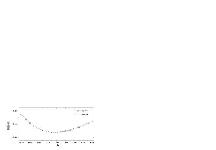
Figure 1: (Color online) Ground state properties of the Sn isotopes. The nuclear binding energies per particle calculated with the DFT approach, discussed in the text, are compared to data from the Audi-Wapstra compilation Audi95 .

The ground state neutron and proton densities are displyed in Fig.2 for several tin isotopes. The comparison between the neutron and proton densities, obtained by HF calculations with the D3Y G-matrix interaction (see Fig.7 from ref.Hofmann ) and the present ones is very reasonable.

Of special importance for our investigation are the surface regions, where the formation of a skin takes place as is visible in Fig.2. For A$\geq$106 the neutron distributions begin to extend beyond the proton density and the effect continues to increase with the neutron excess, up to ${}^{132}Sn$. Thus, these nuclei have a neutron skin. The situation reverses in ${}^{100-102}Sn$, where a tiny proton skin appears.

Figure 2: (Color online) BCS ground state densities of Sn isotopes obtained by the phenomenological DFT approach and used in the QPM calculations.

IV QPM Description of Nuclear Excitations

IV.1 The QPM Hamiltonian

The excitations are calculated in the framework of the Quasiparticle-Phonon Model (QPM) with the model Hamiltonian Sol :

$${H=H_{MF}+H_{M}^{ph}+H_{SM}^{ph}+H_{M}^{pp}}\quad.$$ (36)

Here, $H_{MF}=H_{sp}+H_{pair}$ is the mean-field part, discussed in the previous section. Hence, different from the standard QPM scheme we use single-particle energies and wave functions, obtained self-consistently, according to the procedure described above. For the QPM calculations the pairing part is simplified by using a constant matrix element. The method we have applied for the determination of the ground state properties has been successfully applied for the investigation of low-lying dipole modes in the tin isotopic chain before nadia:2004a ; nadia:2004b and more recently also in the $N=82$ isotones Volz:2006 .

$H_{M}^{ph}$, $H_{SM}^{ph}$ and $H_{M}^{pp}$ are residual interactions, taken as a sum of isoscalar and isovector separable multipole and spin-multipole interactions in the particle-hole and multipole pairing interaction in the particle-particle channels. The latter is included only for the quadrupole and octupole excitations.

Building blocks of the model space are the Quasiparticle-Random-Phase-Approximation (QRPA) phonons:

$$Q^{+}_{\lambda\mu i}=\frac{1}{2}{\sum_{j_{1}j_{2}}{\left(\psi_{j_{1}j_{2}}^{\lambda\mu i}A^{+}_{\lambda\mu}(j_{1}j_{2})-\varphi_{j_{1}j_{2}}^{\lambda\mu i}\widetilde{A}_{\lambda\mu}(j_{1}j_{2})\right)}}$$ (37)

defined as a linear combination of two-quasiparticle creation ${A}^{+}_{\lambda\mu}$ and annihilation operators $\widetilde{A}_{\lambda\mu}$, respectively. The latter is the time reversed operator $\widetilde{A}_{\lambda\mu}=(-)^{\lambda-\mu}A_{\lambda-\mu}$.

Here $j\equiv{(nljm\tau)}$ is a single-particle proton or neutron state.

The (bare) two-quasiparticle operators

$$A^{+}_{\lambda\mu}(j_{1}j_{2})=\left[\alpha^{+}_{j_{1}}\alpha^{+}_{j_{2}}\right]_{\lambda\mu}$$ (38)

are defined by coupling the one-quasiparticle operators to total angular momentum $\lambda$ with projection $\mu$

$$[\alpha^{+}_{j_{1}}\alpha^{+}_{j_{2}}]_{\lambda\mu}=\sum_{m_{1}m_{2}}C^{\lambda\mu}_{j_{1}m_{1}j_{2}m_{2}}\alpha^{+}_{j_{1}m_{1}}\alpha^{+}_{j_{2}m_{2}}$$ (39)

by means of the Clebsch-Gordan coefficients $C^{\lambda\mu}_{j_{1}m_{1}j_{2}m_{2}}=\left\langle j_{1}m_{1}j_{2}m_{2}|\lambda\mu\right\rangle$.

The QRPA states are normalized according to the condition

$$\langle 0|Q_{\lambda\mu i}Q^{+}_{\lambda\mu i}|0\rangle=1,$$ (40)

which can be rewritten in terms of two-quasiparticle weight factors

$$\sum_{j_{1}>j_{2}}{w_{j_{1}j_{2}}(\lambda\mu i)}=1$$ (41)

$$w_{j_{1}j_{2}}({\lambda\mu i})=|\psi_{j_{1}j_{2}}^{\lambda\mu i}|^{2}-|\varphi_{j_{1}j_{2}}^{\lambda\mu i}|^{2}$$

The weight factors $w_{j_{1}j_{2}}({\lambda\mu i})$ are given for some states in Table I and Table II, respectively.

The QRPA operators obey the equation of motion

$$\left[H,Q^{+}_{\alpha}\right]=E_{\alpha}Q^{+}_{\alpha}\quad,$$ (42)

which solves the eigenvalue problem, giving the excitation energies $E_{\alpha}$ and the time-forward and time-backward amplitudes Sol $\psi_{j_{1}j_{2}}^{\lambda i}$ and $\varphi_{j_{1}j_{2}}^{\lambda i}$, respectively.

The QPM Hamiltonian (36) is rewritten in terms of phonons Sol :

$$H=H_{ph}+H_{qph}=\sum_{\lambda\mu i}E_{\lambda i}Q_{\lambda\mu i}^{+}Q_{\lambda\mu i}$$ (43)

$$+\frac{1}{2}\sum_{{\lambda_{1}\lambda_{2}\lambda_{3}}{{{i_{1}i_{2}i_{3}}{\mu_{1}\mu_{2}\mu_{3}}}}}C_{\lambda_{1}\mu_{1}\lambda_{2}\mu_{2}}^{\lambda_{3}{-\mu_{3}}}U_{\lambda_{1}i_{1}}^{\lambda_{2}i_{2}}({\lambda_{3}i_{3}})$$

$$[Q_{\lambda_{1}\mu_{1}i_{1}}^{+}Q_{\lambda_{2}\mu_{2}i_{2}}^{+}Q_{\lambda_{3}-\mu_{3}i_{3}}+h.c.]$$

The first term in the eq.(43) contains free phonon operators and refers to the harmonic part of nuclear vibrations, while the second one is accounting for the interaction between quasiparticles and phonons. The latter reflect in anharmonic effects and fragmentation of the nuclear excitations.

The Hamiltonian (43) is diagonalized assuming a spherical $0^{+}$ ground state which leads to an orthonormal set of wave functions with good total angular momentum JM. For even-even nuclei these wave functions are a mixture of one-, two- and three-phonon components Gri in the following way:

$$\Psi_{\nu}(JM)=\left\{\sum_{i}R_{i}(J\nu)Q^{+}_{JMi}\right.$$ (44)

$$\left.+\sum_{\scriptstyle\lambda_{1}i_{1}\atop\scriptstyle\lambda_{2}i_{2}}P_{\lambda_{2}i_{2}}^{\lambda_{1}i_{1}}(J\nu)\left[Q^{+}_{\lambda_{1}\mu_{1}i_{1}}\times Q^{+}_{\lambda_{2}\mu_{2}i_{2}}\right]_{JM}{+\sum_{{}_{\lambda_{1}i_{1}\lambda_{2}i_{2}\atop\lambda_{3}i_{3}I}}}\right.$$

$$\left.{T_{\lambda_{3}i_{3}}^{\lambda_{1}i_{1}\lambda_{2}i_{2}I}(J\nu)\left[\left[Q^{+}_{\lambda_{1}\mu_{1}i_{1}}\otimes Q^{+}_{\lambda_{2}\mu_{2}i_{2}}\right]_{IK}\otimes Q^{+}_{\lambda_{3}\mu_{3}i_{3}}\right]}_{JM}\right\}\Psi_{0}$$

where R,P and T are unknown amplitudes, and $\nu$ labels the number of the excited states.

The nuclear response on an external electromagnetic field is described in terms of quasiparticles and phonons by a transition operator composed of two parts:

$$M(\mbox{E(M)}\lambda\mu)=M^{ph}(\mbox{E(M)}\lambda\mu)+M^{qph}(\mbox{E(M)}\lambda\mu)$$ (45)

The first part is responsible for the transitions with one-phonon exchange between the initial and final states. The second one contains structures $[\alpha^{+}_{j}\otimes\alpha_{j^{\prime}}]_{\lambda\mu}$ including the interaction between quasiparticles and phonons. It is important for the description of the so-called boson forbidden transitions between nuclear states with the same number of phonons or differing by an even number of them. The corresponding equations of each of the terms could be found in Pon .

IV.2 Transition Densities

In order to understand the character of a nuclear excitation it is useful to consider the spatial structure of the transition. This is accomplished by analyzing the one-body transition densities $\delta\rho(\vec{r})$, which are the non-diagonal elements of the nuclear one-body density matrix. Physically, $\delta\rho(\vec{r})$ corresponds to the density fluctuations, induced by the action of an (external) one-body operator on the nucleus. Hence, the transition densities are directly related to the nuclear response functions and by analyzing their spatial pattern we obtain a very detailed picture of e.g. the radial distribution and localization of the excitation process. The particular usefulness of such an analysis for PDR states was pointed out in Rye02 .

Using the complete set of single-particle states $\varphi_{j}(\vec{r})$ from $H_{MF}$ and a multipole expansion by means of the Wigner-Eckardt theorem, we find the isoscalar (T=0) and isovector (T=1) transition densities in second quantization:

$$\delta\rho^{T}(\vec{r})=\sum_{j_{1}j_{2};\lambda\mu}{\left(i^{\lambda}Y_{\lambda\mu}(\hat{r})\right)^{\dagger}\rho^{\lambda T}_{j_{1}j_{2}}(r)\left[a^{+}_{j_{1}}a_{j_{2}}\right]_{\lambda\mu}}\quad.$$ (46)

For the present purpose we consider non-spin flip transitions of isoscalar and isovector character. The radial parts are given by binomials of radial single-particle wave functions and reduced matrix elements

$$\rho^{\lambda T}_{j_{1}j_{2}}(r)=R^{*}_{j_{1}}(r)R_{j_{2}}(r)\frac{1}{\hat{\lambda}}\langle j_{1}||i^{\lambda}Y_{\lambda}||j_{2}\rangle\langle q|\tau^{T}_{3}|q\rangle\quad,$$ (47)

with $\hat{\lambda}=\sqrt{2\lambda+1}$. The isospin matrix element $\langle q|\tau^{T}_{3}|q\rangle$ is unity for T=0. For an isovector transition we have $\langle q|\tau^{T}_{3}|q\rangle=\pm 1$ for neutrons and protons, respectively.

The transition densities are obtained by the matrix elements between the ground state $|\Psi_{i}\rangle=|J_{i}M_{i}\rangle$ and the excited states $|\Psi_{f}\rangle=|J_{f}M_{f}\rangle$,

$$\rho_{if}^{T}(\vec{r})=\sum_{j_{1}j_{2};\lambda\mu}{\left(i^{\lambda}Y_{\lambda\mu}(\hat{r})\right)^{\dagger}\rho^{\lambda T}_{j_{1}j_{2}}(r)}\langle J_{j}M_{f}|\left[a^{+}_{j_{1}}a_{j_{2}}\right]_{\lambda\mu}|J_{i}M_{i}\rangle$$ (48)

Here, we are interested only in the two-quasiparticle creation and annihilation parts which are given by

$$\Gamma^{+}_{\lambda\mu}(j_{1}j_{2})=\left(u_{j_{1}}v_{j_{2}}+v_{j_{1}}u_{j_{2}}\right)\left(A^{+}_{\lambda\mu}(j_{1}j_{2})+\widetilde{A}_{\lambda\mu}(j_{1}j_{2})\right)$$ (49)

Equation (49) can be rewritten in terms of QRPA phonons defined by the relation (37):

$$\Gamma^{+}_{\lambda\mu}(j_{1}j_{2})=\sum_{i}{g^{\lambda i}_{j_{1}j_{2}}\left(Q^{+}_{\lambda\mu i}+\widetilde{Q}_{\lambda\mu i}\right)},$$ (50)

where

$$g^{\lambda i}_{j_{1}j_{2}}=\frac{\psi_{j_{1}j_{2}}^{\lambda i}+\varphi_{j_{1}j_{2}}^{\lambda i}}{1+\delta_{j_{1}j_{2}}}\left(u_{j_{1}}v_{j_{2}}+u_{j_{2}}v_{j_{1}}\right)$$ (51)

accounts for the BCS and QRPA properties, respectively. Thus, we find

$$\rho_{if}^{T}(\vec{r})=\sum_{j_{1}j_{2};\lambda\mu}{\left(i^{\lambda}Y_{\lambda\mu}(\hat{r})\right)^{\dagger}\rho^{\lambda T}_{j_{1}j_{2}}(r)}\langle J_{f}M_{f}|\Gamma^{+}_{\lambda\mu}(j_{1}j_{2})|J_{i}M_{i}\rangle\quad.$$ (52)

We identify $|J_{i}M_{i}\rangle\equiv|0\rangle$ with phonon vacuum and obtain the excited states by means of the QRPA state operator, eq. (37), $|J_{f}M_{f}\rangle\equiv Q^{+}_{\lambda\mu i}|0\rangle$, which leads us to the commutator relation

$$\rho_{if}^{T}(\vec{r})=\sum_{j_{1}j_{2};\lambda\mu}{\left(i^{\lambda}Y_{\lambda\mu}(\hat{r})\right)^{\dagger}\rho^{\lambda T}_{j_{1}j_{2}}(r)}\langle 0|\left[Q_{\lambda\mu i},\Gamma^{+}_{\lambda\mu}(j_{1}j_{2})\right]|0\rangle\quad.$$ (53)

Hence, in QRPA theory the one-phonon transition density is given by the coherent sum over two-quasiparticle transition densities entering in the structure of a phonon by the relation:

$$\rho_{\lambda i}^{T}(r)=\sum_{j_{1}\geq j_{2}}{\rho_{j_{1}j_{2}}^{\lambda T}(r)g^{\lambda i}_{j_{1}j_{2}}}\quad.$$ (54)

The shape of the transition density defined by eq. (54) is rather strongly correlated with the collectivity of the phonon. For example, the transition densities of the non-collective, two-quasiparticle excitations typically have pronounced maxima inside the nucleus. Those corresponding to the collective transitions with a large number of coherently contributing two-quasiparticle transitions have a maximum at the nuclear surface.

The reduced transition probability $B(E\lambda)$ for the excitation of a state $J_{f}$ from the ground state $J_{i}$ is connected with the transition density with the relation:

$$B(E\lambda)=\frac{2J_{f}+1}{2J_{i}+1}\left[\sum^{1}_{T=0}{e^{\lambda}_{T}\int_{0}^{\infty}r^{\lambda}\rho_{\lambda i}^{T}(r)r^{2}dr}\right]^{2},$$ (55)

where $e^{\lambda}_{T}$ denotes the effective isoscalar and isovector charges, respectively, introduced before.

IV.3 The QPM Model Parameters

Following ref. Vdo ; Bohr the ratio $\kappa^{(\lambda)}_{1}$/$\kappa^{(\lambda)}_{0}$ of the isovector and isoscalar multipole strength parameters, respectively, is assumed to be a constant, independent of the multipolarity $\lambda$. We can find this ratio from the dipole coupling constants by projecting the spurious 1^- state to zero excitation energy and fitting the experimental energy of the Giant Dipole Resonance (GDR)Berman:75 ; Adrich:2005 . For those nuclei, where GDR data are not available the empirical $E^{GDR}_{max}=76/A^{1/3}$ law is used. The E1 transition matrix elements are calculated with recoil-corrected effective charges $q_{n}=-Z/A$ for neutrons and $q_{p}=N/A$ for protons, respectively, as discussed in sect. II ^[3].

V Results for the Dipole Response

V.1 General Features of the Dipole Response

The dependence of the calculated total PDR strength ($\sum B(E1)\uparrow$) on the mass number for the whole chain of isotopes ^100-132Sn is shown in Fig.3 and compared to the skin thickness $\delta r$, eq. (10) of these nuclides. Here the sum is taken over QRPA dipole states presented in Table 1 and Table 2, respectively. According to state vectors structure they have been associated with PDR. These results illustrate and confirm the conclusion drawn in sect. II and as already stated in previous work nadia:2004a establish the close relationship of the PDR strength and the skin thickness.

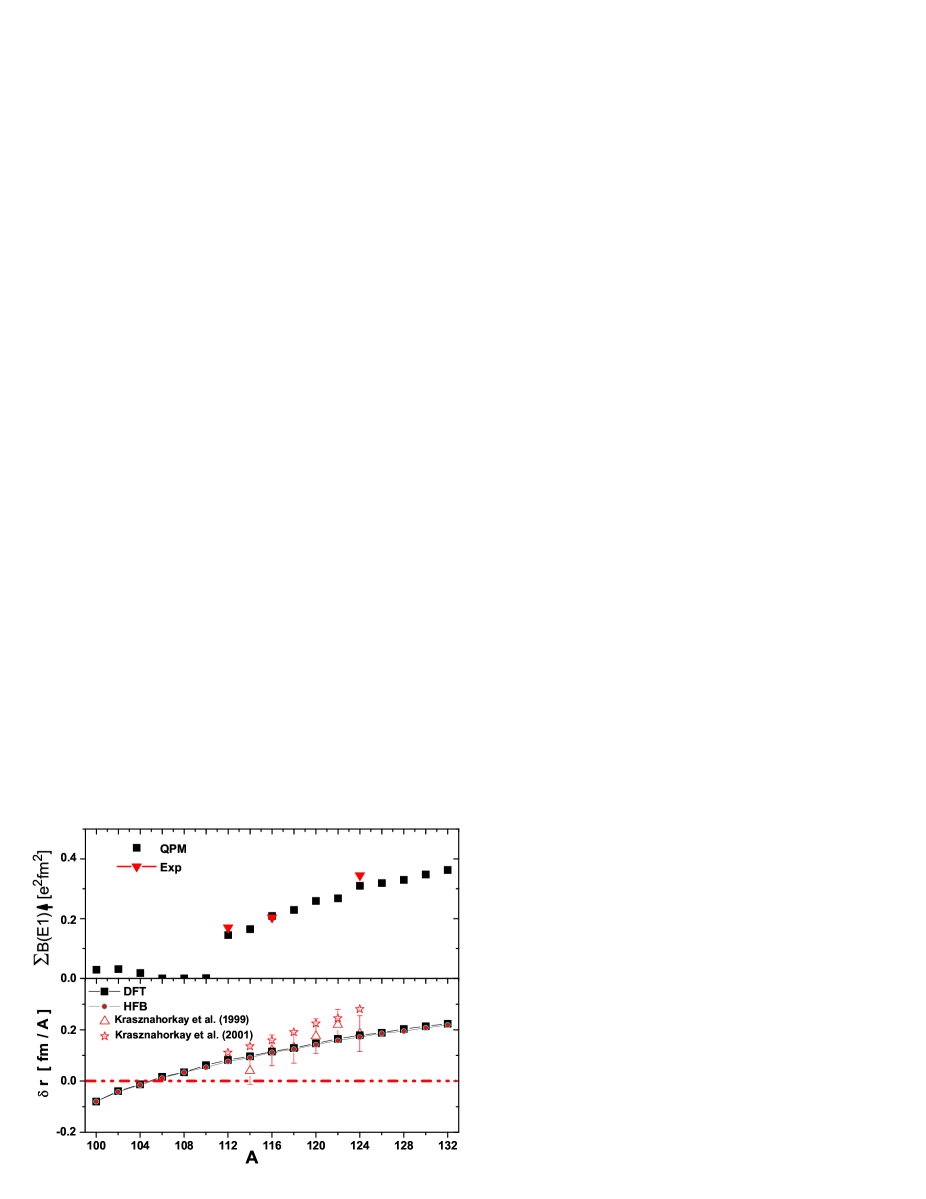
Figure 3: (Color online) QPM results for the total PDR strengths in the ^100-132Sn isotopes (upper panel) are displayed for comparison together with the nuclear skin thickness $\delta r$, eq. (10) (lower panel). Experimental data on the total PDR strengths in ¹¹⁶Sn and ¹²⁴Sn ref.Govaert98 and ¹¹²Sn Ozel are also shown. In the lower panel, the skin thickness derived from charge exchange reactions by Krasznahorkay et al. Sn-skin1 ; Sn-skin2 are indicated.

In the region between ^110-132Sn the total PDR strength increases smoothly with the neutron number. This establishes a clear correlation of the total PDR strength and the thickness of the neutron skin in these nuclei, thus confirming our previous results nadia:2004a ; nadia:2004b ; Volz:2006 and the more recent investigations for several $N=82$ isotones Volz:2006 . The close relationship between $\delta r$ and the PDR modes is underlined by the result, that the PDR becomes negligibly small in the region ^106-108Sn, where $\delta r$ changes sign (see Fig.3). In these isotopes the lowest-lying states carry the characteristics of the low-energy branch of the GDR as indicated by the structure and shape of the transition densities.

From the QRPA calculations in ^110-132Sn a sequence of low-lying one-phonon 1^- states at excitation energies $E^{*}=6-7.5$ MeV of almost pure neutron structure is obtained with a minor fraction of protons less than 1%. The structure of the state vectors is indicated in Table I. The most important part of the total PDR strength comes from the excitations of the least bound neutrons from the 3s- and 2p- and 2d-subshells. Some other neutron orbitals of significance for the size of the neutron skin are $1h_{11/2}$ and $1i_{13/2}$, which have an important contribution to the PDR transition matrix elements in ¹³²Sn nuclei, for example.

The dominant neutron structure and remarkable stability of the wave functions of the low-lying one-phonon 1^- states in these nuclei is in agreement with our previous findings on the PDR mode in ^120-132Sn isotopes nadia:2004a and N=82 Volz:2006 isotones.

Towards the lighter Sn isotopes the average energy of the excited dipole states increases, while their total number decreases (see Table I). The dependence of the PDR energy on the neutron excess is connected with the one-neutron separation energy, decreasing gradually towards the heavier tin isotopes. Such a tendency has been observed also experimentally in N=82 isotones (see ref. Tonchev:2007 ).

An exception is the double magic ¹³²Sn nucleus, in which the PDR centroid energy is $E^{*}=7.1MeV$ and is still below the neutron emission threshold. The present result in ¹³²Sn is slightly different from our previous one nadia:2004a ; nadia:2004b due to minor readjustments in the single-particle spectrum.

In ^100-104Sn the lowest dipole excitations, E^∗= 8.1-8.3 MeV, are dominated by proton excitations. The structure of the QRPA state vectors and B(E1) transition probability are given in Table II. There it is seen, that configurations involving quasibound $2p_{3/2}$ and $1g_{9/2}$ proton states confined by the Coulomb barrier are the major components. This is a remarkable Coulomb effect enlightening the delicate balance among various effects as a prerequisite for a PDR and, by comparison to Fig. 2, the existence of a nuclear skin. From Fig. 2 it is seen, that this is the mass region, where the neutron skin turns into a proton skin. In agreement with the considerations in sect. II the vanishing skin is accompanied by a strong suppression of the dipole strength. The smallest strength is found at $A=110-112$, which is slightly above the turnover point of $\delta r$ at $A=106$. This delay is caused by Coulomb effects, which enhance the dipole response from weakly bound proton orbitals in that mass region over the values to be expected for full isospin symmetry.

Electromagnetic breaking of isospin symmetry is also the main reason for the persisting of low-energy dipole strength close to ¹⁰⁰Sn. Already the quite different behavior is an indication for another mechanism underlying these excitations. There, at $N=Z$ the isoscalar dipole charge vanishes, hence the electromagnetic operator by itself does no longer support isoscalar transition. However, Coulomb effects in the single-particle wave functions translate into an intrinsic isospin symmetry breaking on the level of matrix elements. The mechanism behind a neutron skins in the heavy Sn isotopes is a strong interaction effect, namely the repulsive action of the isovector self-energy to the neutron mean-field. In neutron-rich nuclei the isovector self-energy adds attractively to the proton potential, which partially compensates the Coulomb repulsion. Because for N$\to$Z the isovector self-energy becomes negligible the proton skins seen in the light Sn isotopes must be of a different origin. In fact, they are due to the Coulomb potential. Towards $N=Z$ the Coulomb interaction can act in full strength on the protons, pushing them apart and leading to a rearrangement of a certain fraction of the nuclear charge in the surface region.

The average energies in Table I and Table II have been obtained by the relation $\left\langle E\right\rangle=\sum_{i}E_{i}B_{i}/\sum_{i}B_{i}$, where $E_{i}$ and $B_{i}$ are the QRPA energies and reduced transition probabilities, respectively.

V.2 PDR and GDR Transition Densities

For a more detailed insight into the characteristic features of the dipole excitations we consider the evolution of the proton and neutron transition densities for in the various energy regions. In Fig.4 and Fig.5 we display the QRPA transition densities for several $N=82$ isotones in and the $Z=50$ isotopes ^112,122,132Sn for three different regions of excitation energies: the low-energy PDR region below the neutron emission threshold, the transitional region up to the GDR and in the GDR region and beyond⁴. The transition densities displayed in Fig.4, Fig. 5 and Fig. 6 were obtained by summing over the transition densities of the individual one-phonon states located in the energy intervals denoted at the top of each column of the figures, i.e.

$$\rho_{\lambda}^{T}(r)=\sum_{i}\rho_{\lambda i}^{T}(r).$$ (56)

$\rho_{\lambda i}^{T}(r)$ is determined by equation (54), where the module and the phases are unambiguously determined by our microscopic approach. The neutron and proton transition densities are then obtained by taking half the difference and the sum of the isoscalar and isovector pieces, respectively.

A common features of the all cases presented in Fig.4 is that up to $E^{*}=8.1$ MeV the protons and neutrons oscillate in phase in the nuclear interior, while at the surface only neutron transitions contribute. The same behavior of the neutron and proton transition densities is observed below 8 MeV for tin isotopes (see Fig.5). This pattern is generic to the lowest dipole states making it meaningful to distinguish these excitations from the well known GDR states. Hence, we are allowed to identify the PDR states with a new mode of nuclear excitation, not seen in stable $N\sim Z$ nuclei.

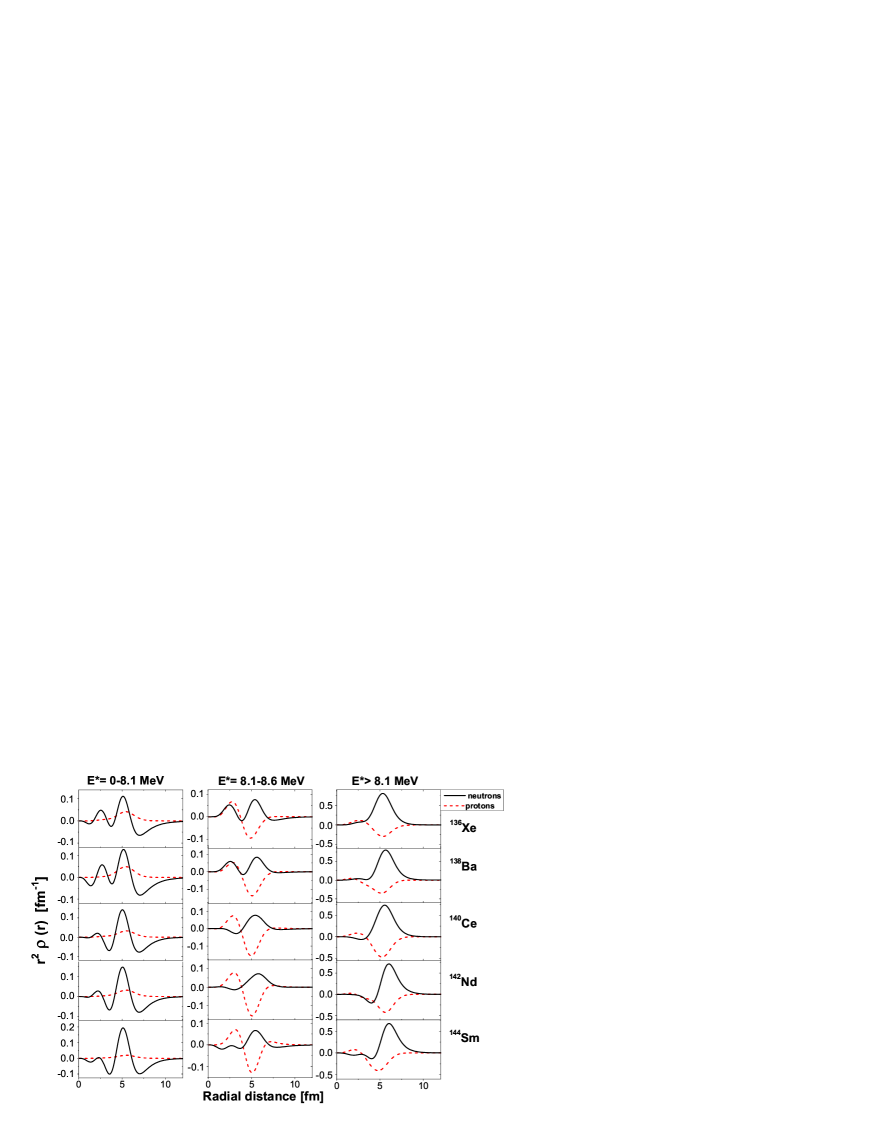
Figure 4: (Color online) QRPA results for the one-phonon dipole transition densities in N=82 nuclei.

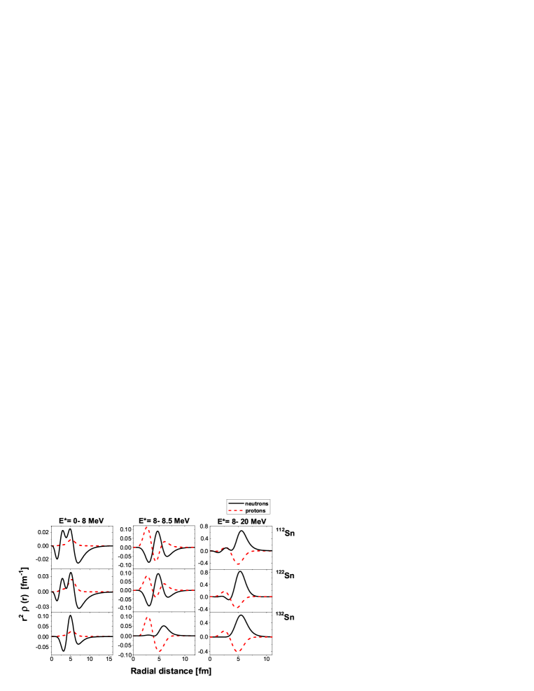
Figure 5: (Color online) QRPA results for the one-phonon dipole transition densities in ^112,122,132Sn nuclei.

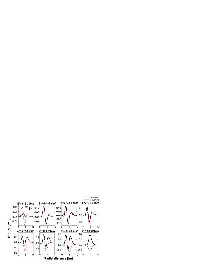
Figure 6: (Color online) QRPA results for the one-phonon dipole transition densities in ¹⁰⁰Sn.

In the energy region $E^{*}=8.1-8.6$ MeV for N=82 isotones and 8-8.5 MeV for Z=50 respectively, the transition densities suddenly change. Rather abruptly, protons and neutrons start to oscillate out of phase over the whole nuclear volume as known from the GDR. Thus, we are encountering the low-energy part of the GDR, although the strengths of these two different type of excitations, the PDR and the low-energy GDR tail are quite comparable. Also energetically they are located very close to each other. This makes the task to distinguish the two modes rather demanding. Theoretically, we can always use the transition densities for a detailed analysis and a precise identification of the mode although a corresponding experimental measurement will not be feasible for the foreseeable future. Finally, we show in Fig.4 and Fig.5 the one-phonon QRPA proton and neutron transition densities for the states at $E^{*}>8.1$ MeV and $E^{*}>8$ MeV, respectively. A pronounced isovector oscillation of protons against neutrons, peculiar to the GDR, is observed. The latter, as a very collective mode, has a strength one order of magnitude larger than the PDR.

We have pointed out the special character of the low-energy dipole excitations in the ^100-104Sn isotopes. This is reflected also in the transition densities. In ¹⁰⁰Sn, Fig.6, proton oscillations prevail below $E^{*}<8.4$ MeV. In the nuclear interior isoscalar, or mixed symmetry vibrations of protons and neutrons are found, while at the surface only protons contribute. Hence, this mode could be related to a proton skin excitations. In the energy region $E^{*}=8.4-9.2$ MeV oscillations of weakly bound neutrons from the surface region take place. The behaviour of the transition densities and the structure of the $1^{-}$ states at these energies is similar to the neutron PDR mode identified in the more neutron rich tin isotopes (see Fig.5 as well). At energies $E^{*}>9.2$ MeV the low-energy tail of the GDR is encountered. The last plot in Fig.6 displays the neutron and proton transition densities summed over the GDR region, $E^{*}=9.2-20$ MeV.

The QRPA calculations on the neutron and proton PDR and the GDR strength distributions at excitation energies up to 20 MeV in several thin isotopes in the mass region ¹⁰⁰Sn$\div^{132}$Sn are presented in Fig.(7). An interesting feature we have observed is that between the N=50 and N=82 closed shells with the increase of the neutron number from ¹⁰⁰Sn toward ¹³²Sn the PDR strength is shifted to lower excitation energies relatively to the GDR mode, which is almost unchanged. This can be explained with a strong correlation between the PDR excitation energy and the energy of the neutron threshold, which also decreases in the same direction.

Table 1: Energy, B(E1) values and wave functions of the first QRPA 1^- states in the ^110÷132Sn isotopes. Only the dominant neutron and proton components are given. Neutron and proton configurations are denoted by the indices $\nu$ and $\pi$, respectively.

Nucleus	State	Energy	Structure	B(E1)$\uparrow$	$<E>$
	J${}_{\nu}^{\pi}$	[MeV]	$w_{j_{1}j_{2}}$, $\%$	[e2fm2]	[MeV]
110Sn	1${}_{1}^{-}$	7.834	99.9$\%[1g_{7/2}2f_{7/2}]\nu$	0.001	7.8
112Sn	1${}_{1}^{-}$	7.509	99.8$\%[1g_{7/2}2f_{7/2}]\nu$	0.001
	1${}_{2}^{-}$	7.906	99.0$\%\left[3s_{1/2}3p_{3/2}\right]\nu$	0.144	7.9
114Sn	1${}_{1}^{-}$	7.329	99.8$\%[1g_{7/2}2f_{7/2}]\nu$	0.001
	1${}_{2}^{-}$	7.665	99.2$\%\left[3s_{1/2}3p_{3/2}\right]\nu$	0.159	7.7
	1${}_{3}^{-}$	8.021	99.9$\%\left[2d_{3/2}3p_{3/2}\right]\nu$	0.005
116Sn	1${}_{1}^{-}$	6.974	99.7$\%[2g_{7/2}3f_{7/2}]\nu$	0.001
	1${}_{2}^{-}$	7.188	99.$\%\left[3s_{1/2}3p_{3/2}\right]\nu$	0.199	7.2
			+ 0.1$\%\left[1g_{9/2}1h_{11/2}\right]\pi$
	1${}_{3}^{-}$	7.391	99.9$\%\left[2d_{3/2}3p_{1/2}\right]\nu$	0.009
118Sn	1${}_{1}^{-}$	6.904	99.6$\%[1g_{7/2}2f_{7/2}]\nu$	0.001
	1${}_{2}^{-}$	7.054	98.1$\%\left[3s_{1/2}3p_{3/2}\right]\nu$	0.208	7.1
			+ 0.1$\%\left[1g_{9/2}1h_{11/2}\right]\pi$
	1${}_{3}^{-}$	7.098	99.1$\%\left[2d_{3/2}3p_{3/2}\right]\nu$	0.02
120Sn	1${}_{1}^{-}$	6.795	99.6$\%[2d_{3/2}3p_{3/2}]\nu$	0.009
	1${}_{2}^{-}$	6.870	95.2$\%\left[1g_{7/2}2f_{7/2}\right]\nu$	0.014	6.9
	1${}_{3}^{-}$	6.910	94$\%\left[3s_{1/2}3p_{3/2}\right]\nu$	0.238
			+ 0.1$\%\left[1g_{9/2}1h_{11/2}\right]\pi$
122Sn	1${}_{1}^{-}$	6.469	99.8$\%[2d_{3/2}3p_{3/2}]\nu$	0.014
	1${}_{2}^{-}$	6.710	95.3$\%\left[3s_{1/2}3p_{3/2}\right]\nu$	0.245	6.7
			+ 0.1$\%\left[1g_{9/2}1h_{11/2}\right]\pi$
	1${}_{3}^{-}$	6.754	95.8$\%\left[1g_{7/2}2f_{7/2}\right]\nu$	0.009
			+ 0.1$\%\left[1g_{9/2}1h_{11/2}\right]\pi$

			Table I continued
124Sn	1${}_{1}^{-}$	6.359	99.8$\%[2d_{3/2}3p_{3/2}]\nu$	0.017
	1${}_{2}^{-}$	6.702	94.8$\%\left[3s_{1/2}3p_{3/2}\right]\nu$	0.284	6.68
			+ 0.1$\%\left[1g_{9/2}1h_{11/2}\right]\pi$
	1${}_{3}^{-}$	6.749	95.6$\%\left[1g_{7/2}2f_{7/2}\right]\nu$	0.009
			+ 0.1$\%\left[1g_{9/2}1h_{11/2}\right]\nu$
126Sn	1${}_{1}^{-}$	6.180	99.7$\%[2d_{3/2}3p_{3/2}]\nu$	0.019
	1${}_{2}^{-}$	6.621	51.4$\%\left[3s_{1/2}3p_{3/2}\right]\nu$	0.163	6.6
			+ 48.3$\%\left[1g_{7/2}2f_{7/2}\right]\nu$
	1${}_{3}^{-}$	6.642	51.5$\%\left[1g_{7/2}2f_{7/2}\right]\nu$	0.137
			+ 47.$\%\left[3s_{1/2}3p_{3/2}\right]\nu$
			+ 0.2$\%\left[1g_{9/2}1h_{11/2}\right]\pi$
128Sn	1${}_{1}^{-}$	5.611	99.7$\%[2d_{3/2}3p_{3/2}]\nu$	0.023
	1${}_{2}^{-}$	6.201	97.8$\%\left[3s_{1/2}3p_{3/2}\right]\nu$	0.306	6.2
			+ 0.2$\%\left[1g_{9/2}1h_{11/2}\right]\pi$
	1${}_{3}^{-}$	6.352	99.1$\%\left[1g_{7/2}2f_{7/2}\right]\nu$	0.001
130Sn	1${}_{1}^{-}$	5.172	99.7$\%[2d_{3/2}3p_{3/2}]\nu$	0.028
	1${}_{2}^{-}$	5.882	98.1$\%\left[3s_{1/2}3p_{3/2}\right]\nu$	0.319	5.8
			+ 0.2$\%\left[1g_{9/2}1h_{11/2}\right]\pi$
	1${}_{3}^{-}$	6.114	99.4$\%\left[1g_{7/2}2f_{7/2}\right]\nu$	0.0002
132Sn	1${}_{1}^{-}$	5.754	99.7$\%[1g_{7/2}2f_{7/2}]\nu$	0.0001
	1${}_{2}^{-}$	7.109	88.6$\%\left[2d_{5/2}2f_{7/2}\right]\nu$	0.363	7.1
			+ 10.8$\%\left[1h_{11/2}1i_{13/2}\right]\nu$
			+ 0.2$\%\left[1g_{9/2}1h_{11/2}\right]\pi$

Table 2: The same as Table I for ^100÷104Sn isotopes.

Nucleus	State	Energy	Structure	B(E1)$\uparrow$		$<E>$
	J${}_{\nu}^{\pi}$	[MeV]	$w_{j_{1}j_{2}}$,$\%$	[e2fm2]		[MeV]
100Sn	1${}_{1}^{-}$	8.032	99.5$\%[1f_{5/2}2d_{5/2}]\nu$	0.001
	1${}_{2}^{-}$	8.292	82.1$\%\left[2p_{3/2}2d_{5/2}\right]\pi$	0.028		8.29
102Sn	1${}_{1}^{-}$	8.174	82.6$\%[2p_{3/2}2d_{5/2}]\pi$	0.031
104Sn	1${}_{1}^{-}$	8.256	80.8$\%[2p_{3/2}2d_{5/2}]\pi$	0.016

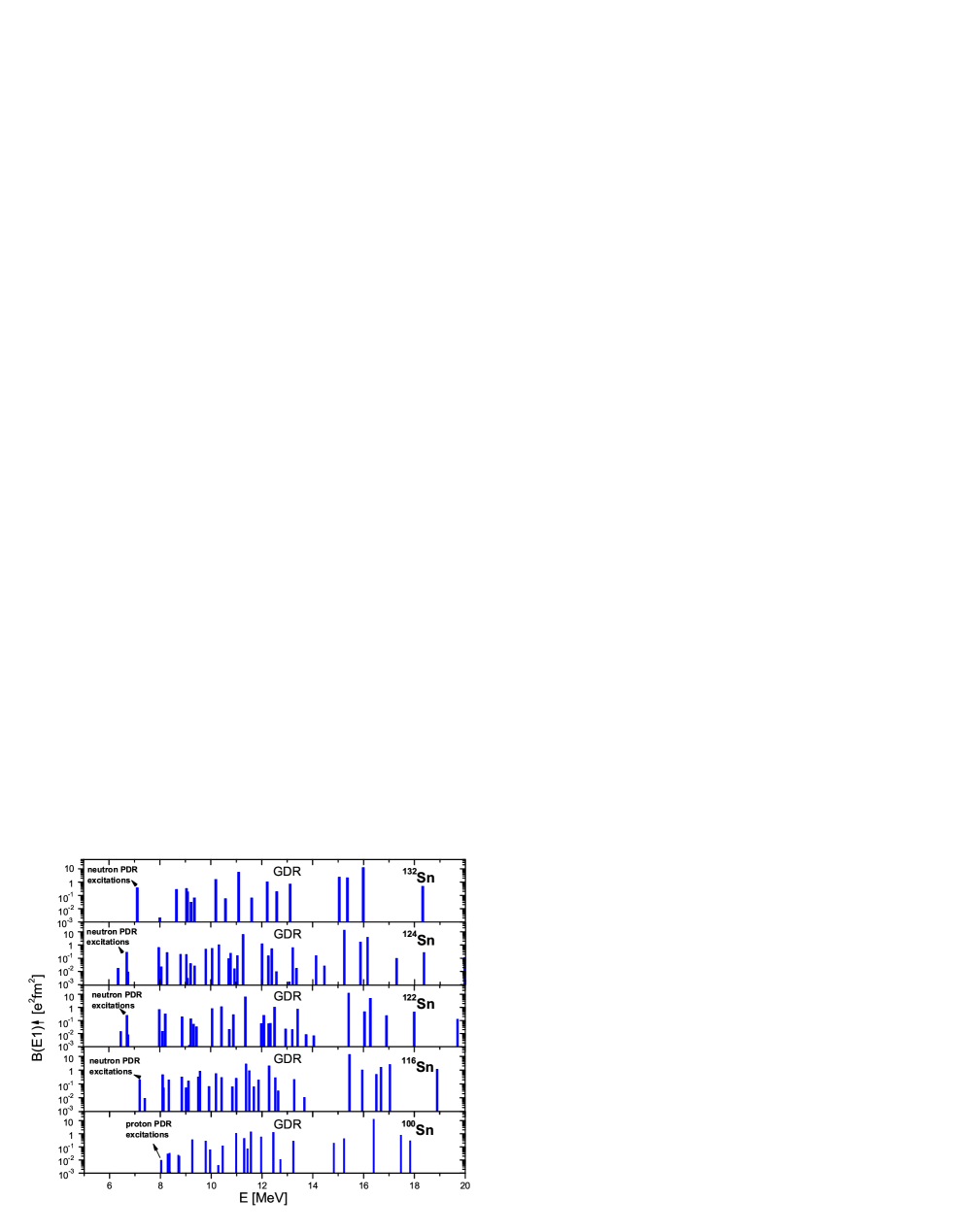
Figure 7: (Color online) QRPA results for the PDR and GDR strength distributions in ^{100,116,122,124,132}Sn isotopes.

V.3 Multi-phonon effects in the low-energy dipole spectra of ¹²⁴Sn.

In the multi-phonon QPM calculations the structure of the excited states is described by wave functions as defined in eq. 44.We now investigate multi-phonon effects using a model space with up to three-phonon components, built from a basis of QRPA states with J${}^{\pi}=1^{\pm},2^{+},3^{-},4^{+},5^{-},6^{+},7^{-},8^{+}$. Since the one-phonon configurations up to $E^{*}$=20 MeV are considered the core polarization contributions to the transitions of the low-lying 1^- states are taken into account explicitly. Hence, we do not need to introduce dynamical effective charges. In the excitation energy interval up to $E^{*}$=9 MeV we use a total of about 250 multi-phonon configurations.

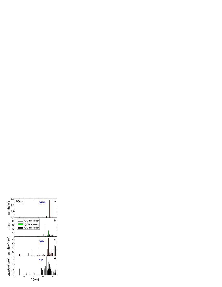
Figure 8: (Color online) Electromagnetic dipole response in ¹²⁴Sn from: a/QRPA calculations; c/QPM with up to three-phonon configuration space including 250 components; d/experimental data from Govaert98 up to excitation energies $E^{*}$=7.5 MeV. Distributions of the PDR QRPA phonons over the 1^- excited states is presented in Fig 10.b.

The results for the dipole response below the neutron threshold in ¹²⁴Sn are presented in Fig.8. By comparing Fig.8a and Fig.8c it is seen that the pure two-quasiparticle QRPA strengths is strongly fragmented once the coupling to multi-phonon configurations is allowed. As found previously the lowest-lying 1^- state without a QRPA counterpart is predominantly given by a two-phonon quadrupole-octupole excitation PDRrev:06 . The $[2^{+}_{1}\otimes 3^{-}_{1}]$ configuration accounts for 85% of the QPM wave function. The $1^{-}_{1}$ state is located at $E^{*}=3.50$ MeV, carrying a reduced transition probability $B(E1;g.s\rightarrow 1^{-}_{1})=6.06$ $10^{-3}$ $e^{2}fm^{2}$. The values are in a good agreement with the experiment ($E^{*}=3.49$ MeV and $B(E1;g.s\rightarrow 1^{-}_{1})=6.08$ $10^{-3}$ $e^{2}fm^{2}$ Bry and previous QPM calculations refs.Bry ; nadia:2004a .

Here, our attention is especially focused on the 1^- states above the two-phonon dipole state and below the neutron threshold. From the analysis of the QRPA calculations discussed above the 1^- states presented in Fig.8a are PDR modes. Their fragmentation over the multi-phonon 1^- excited states are shown in Fig.8b. From that plot we can determine the energy region, where the PDR is located. In the particular case of ¹²⁴Sn in the interval $E^{*}\leq 7.5$ MeV is exhausted about 80$\%$ of the total one-phonon PDR strength.

Comparing the fragmentation pattern of the theoretical low-energy dipole strength in ¹²⁴Sn to recent measurements Bry ; Govaert98 , displayed in Fig.8d, we find that the three-phonon QPM results are still not fully accounting for the observed distribution, although we have increased the number of the multi-phonon configurations twice in comparison with our previous calculations from nadia:2004a . However, the calculated total QPM dipole strength in the PDR energy range $E^{*}=5.7-7.2$ MeV is $\sum B(E1)_{QPM}=0.324$ $e^{2}fm^{2}$ which is almost identical to the experimentally deduced strength, $\sum B_{exp}(E1)=0.345(43)e^{2}fm^{2}$.

The good overall agreement between the calculations and the experiment Govaert98 for the total PDR strength and centroid energy in ¹²⁴Sn indicates that in this particular case the main PDR properties could already be determined on the level of the one-phonon approximation. A similar conclusion was drawn in our previous QPM calculations for several Sn isotopes with A=120-130 nadia:2004a . An important observation is that the low-energy tail of the GDR can give a strong contribution to the dipole strength around the particle threshold. This effect appears because the GDR states may overlap with the PDR region and can be fragmented due to coupling to multi-phonon states. The effect becomes increasingly important in nuclei where the neutron threshold is higher, hence approaching the GDR region, as in the lighter Sn isotopes or ¹³²Sn, where the PDR strength is situated very close to the neutron threshold. Such a situation demands much larger model spaces.

VI Other Model Calculations and Experimental Data

VI.1 PDR Models

Overall, the present Sn results are in, at least qualitative, agreement with the theoretical PDR investigations by Density Functional Theory (DFT) Cha94 , relativistic RPA Piek , relativistic QRPA Vret01 ; Paar , extended theory of finite Fermi systems THartmann and QRPA-PC (Quasiparticle Random Phase Approximation plus Phonon Coupling)Sarchi . They confirm the conclusions drawn from our former QPM calculations in ²⁰⁸Pb Rye02 and for the N=82 case, studied recently in Volz:2006 . All these different approaches confirm the PDR mode as a universal low-energy dipole mode of a character generic for isospin asymmetric nuclei.

As an example we cite the studies of ref.Cha94 investigating low-lying dipole states in ^40-48Ca in a density functional theory approach. Similar to the much heavier nuclei considered here the PDR is predicted to be located in the energy range 5-10 MeV. Also in that nucleus, the centroid energy of the PDR strength is found to decrease with the number of the neutrons, while the integrated PDR strength (below the neutron particle emission threshold) increases. These results agree with the present calculations and our findings in refs. nadia:2004a ; nadia:2004b ; Volz:2006 in the Sn isotopes. A common result of all model calculations discussed here is a clear connection between the existence of low-energy dipole strength and the presence of isospin assymetry or nuclear skin in the investigated nuclei. However, we emphasize, that arguments based on the energy alone are likely to be insufficient for a unambiguous identification of the dipole states as belonging to the PDR. To our understanding, as an important conclusion from the analysis of the transition densities, the PDR strength is attached only to the states located below the neutron particle emission threshold. Hence, the centroid of the PDR energy has a tendency to be closely connected with the one-neutron separation energy. At higher energies, the dipole spectrum merges rapidly into the low energy tail of the GDR and the transitions lose their characteristic PDR features.

A controversial question is the degree of the collectivity of the PDR transitions. This issue has been discussed by several authors Cha94 ; Piek ; Vret01 ; Sarchi ; Paar07 . In the non-relativistic models like ours Rye02 ; nadia:2004b ; Volz:2006 and QRPA-PC for example, the PDR is referred to as the excitation of two-quasiparticles states. In ¹³²Sn the relativistic QRPA Vret01 predicts a collective neutron state at $E^{*}=8.6$ MeV that has been related to the PDR excitation. This state contains particle-hole configurations accounting for transitions into continuum states. The collectivity of such excitations we found to dependent strongly on the choice of the spin-orbit potential affecting the energy gap between the bound hole and unbound particle region by shifting the continuum states. Our standard choice for the spin-orbit potential strength Tak , otherwise describing the spectra reasonably well, disfavors such admixtures.

Experimental data for low-energy dipole states below the particle emission threshold are available for a number of Sn isotopes, ¹¹⁶Sn and ¹²⁴Sn Govaert98 and recent measurements in ¹¹²Sn Ozel , and for several N=82 isotones Volz:2006 . Altogether, our calculations describe these data quite satisfactory.

VI.2 Dipole Response in ^130,132Sn

We pay special attention to the region around ¹³²Sn, because of the expected closure of the N=82 neutron shell as indicated e.g. by the energy of the first $2^{+}$ state. The HFB calculations predict a double shell closure for protons and neutrons, respectively. On the other hand, the HFB calculations show, that the N=82 neutron shell closure depends to some extent on the balance between spin-orbit splitting and the effective pairing strength.

The LAND-FRS collaboration at GSI has recently measured in a pioneering Coulomb dissociation experiment the dipole response above neutron threshold in ^130,132Sn Adrich:2005 . These measurements are providing the first data on the dipole response in the these exotic nuclei. However, we have to be aware, that any dipole strength below the particle emission threshold – if existing – cannot be accessed by this type of measurement. Besides the GDR a prominent feature of the data is a resonance-like structure around $E^{*}\sim$10 MeV exhausting a few percent of the EWSR in ^130,132Sn nuclei. In Adrich:2005 this part of the response function was interpreted as a PDR. We compare our calculated integrated dipole photoabsorption cross sections $\sigma$ in the Sn isotopes to the LAND-FRS data Adrich:2005 ) in Table 3.

A different conclusion is obtained by analyzing our QRPA wave functions and the dipole transition densities. In ^130,132Sn, we find dipole excitations, carrying the characteristic features of PDR transitions, below the neutron particle emission threshold, as indicated in the first three columns of Table 3 and in Fig.7. In the energy domain $E^{*}=8-12$ MeV, assigned in Adrich:2005 as PDR region, we obtain in both nuclei another concentration of E1 strength (see also Fig. 7). However, because the transition densities show the GDR-type behavior, we consider this part of the dipole response as the low-energy tail (LET) of the GDR. Although the LET evolves in close relation to the neutron excess, but it does not seem to be related to excitations of the neutron skin.

In fact, there is a simple proportionality between the dipole photoabsorption cross section, integrated over an energy interval around $E^{*}$, and reduced transition strength, $\int{dE\sigma_{\gamma}}\sim E^{*}B(E1,E^{*})$, up to a numerical factor Bohr . Exploiting this relation, we have calculated the integrated dipole photoabsorption cross sections in the LET regions of ^130,132Sn. In Tab.3 it is seen that the theoretical results agree rather well with those determined experimentally in Adrich:2005 . Within the experimental error bars, also the full strengths, including excitations up to 20 MeV, are reasonably well described.

Table 3: Dipole response in ^130,132Sn. Calculated energies and integrated cross sections (columns denoted by QPM) in one-phonon approximation are compared with recent measurements (columns denoted by Exp.) Adrich:2005 of PDR and GDR in Sn isotopes. The calculated integrated PDR and low-energy GDR cross sections are denoted by $\int\sigma^{PDR}$ and $\int\sigma_{LET}^{GDR}$, respectively. The total photoabsorption cross section up to 20 MeV is denoted by $\int\sigma^{GDR}$

. Nucl. PDR $\left\langle E\right\rangle_{PDR}$ $\int\sigma^{PDR}$ $E_{max}^{PDR}$ $\int\sigma^{PDR}$ $E^{GDR}_{LET}$ $\int\sigma^{GDR}_{LET}$ $E_{GDR}^{max}$ $E_{GDR}^{max}$ $\int\sigma^{GDR}$ $\int\sigma^{GDR}$ $(^{Energy}_{region})$ [MeV] [mb MeV] [MeV] [mb MeV] [MeV] [mb MeV] [MeV] [MeV] [mb MeV] QPM QPM QPM Exp. Exp. QPM QPM Exp. QPM Exp. QPM ¹³⁰Sn 0-7.4 5.8 8.2 10.1(7) 130(55) 8-11 137.3 15.9(5) 16. 1930(300)* 1616 ¹³²Sn 0-8 7.1 10.4 9.8(7) 75(57) 8-11 97.6 16.1(7) 16.1 1670(420)* 1518

For the purpose of a realistic description of the measured spectra, we have applied a slightly different numerical method by solving the QRPA Dyson equation similar to the approach used in PhysRep:97 allowing to take into account explicitly the continuum decay width $\Gamma^{\uparrow}$ of the states above particle threshold, ranging from a few keV up to about hundred keV. Still, a comparison to the LAND-FRS spectra is only possible after folding the theory with the experimental acceptance filters Adam:2007 . The results of such calculations is shown in Fig. 9 and Fig.8 with a quite remarkable agreement to the data.

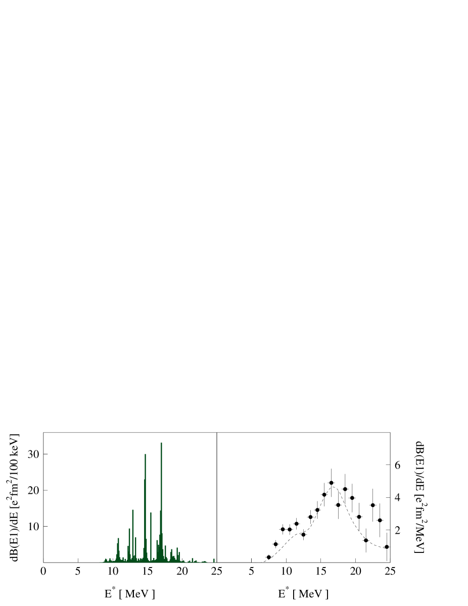
Figure 9: Electromagnetic QRPA dipole response function and LAND-FRS data Adrich:2005 for ¹³⁰Sn. The QRPA results (left), where obtained by solving the Dyson equation and include the decay widths from particle emission. In the right panel the theoretical response function has been folded with the experimental acceptance filter Adam:2007 (dashed line) and is compared to the data (symbols).

Figure 10: Electromagnetic QRPA dipole response function and LAND-FRS data Adrich:2005 for ¹³²Sn. As in Fig. 9 the QRPA results (left) include the decay widths from particle emission. In the right panel the theoretical response function has been folded with the experimental acceptance filter Adam:2007 (dashed line) and is compared to the data (symbols).

VII Summary and Conclusions

Low-energy dipole excitations in ${}^{100-132}Sn$ isotopes were studied by a theoretical approach based on HFB and QPM theory. From our calculations in ¹¹²Sn $\div$ ¹³²Sn we obtained low-energy dipole strength in the energy region below 8 MeV, close but below the neutron emission threshold. These states are of a special character. Their structure is dominated by neutron components and their transition strength is directly related to the presence of a neutron skin. Their generic character is further confirmed by the shape and structure of the related transition densities, showing that these pygmy dipole resonances (PDR) are clearly distinguishable from the conventional GDR mode. Our calculations show a rather abrupt transition from PDR- to the GDR-type excitations, typically occurring at energies slightly above the particle threshold. An important finding in our calculations is that an accurate description of the PDR part of the dipole spectrum requires a single particle spectrum corresponding to a total effective mass $\frac{m^{*}}{m}=1$. From that observation we conclude that non-localities and dynamical effects form core polarizations are important for a proper description of the PDR spectrum. Pure HF and HFB models, whether non-relativistic or relativistic, typically use effective masses considerably less then unity. Hence, such approaches might miss important effects.

In the most proton-rich exotic nuclei ^100-104 Sn the lowest dipole states are almost pure proton excitations. They are related to oscillations of weakly bound protons, indicating a proton PDR. The interesting point is, that we found these states in heavy nuclei with N slightly larger, or equal to Z. We suggest, that the effect is due to Coulomb repulsion, that pushes out weakly bound protons orbitals to the nuclear surface. Coulomb effects also induce a considerable amount of isospin breaking at the level of single-particle wave functions.

Since similar observation have been made in the nearby $N=82$ isotonic nuclei, we may conclude, that the features discussed here are indicating a new universal mode of excitation. It is worthwhile to extent the investigations also in other mass regions. Promising candidates are the Ni and Ca isotopes, but also the light mass region, where a mixing between halo and skin degrees of freedom can be expected, which may lead to still other modes of excitations.

Acknowledgements

This work was supported by DFG contract Le-439/6 and GSI. We are grateful to Adam Klimkiewicz for providing us with experimental results of the photoabsorption cross sections in ^130,132Sn and his support in performing the folding with the LAND-FRS acceptance filter and providing the figures. We thank to R.V. Jolos for his attention to the paper and the discussions.

Appendix A The Rearrangement Potentials

Once the proton and neutron self-energies $\Sigma_{p,n}(\rho)$, respectively, are known the rearrangements parts are determined and properly subtracted by exploiting relations found in infinite nuclear matter. In symmetric nuclear matter with $\rho_{p}=\rho_{n}$ we find for the isoscalar self-energy $\Sigma_{0}=(\Sigma_{n}+\Sigma_{p})/2$ the relation

$$\Sigma_{0}(\rho)=\frac{1}{2}\frac{\partial}{\partial\rho}\rho U_{0}(\rho),$$ (57)

which we integrate to give

$$U_{0}(\rho)=\frac{2}{\rho}\int^{\rho}_{0}{d\rho^{\prime}\Sigma_{0}(\rho^{\prime})}\quad,$$ (58)

providing us with $U_{0}(\rho)=(U_{n}(\rho)+U_{p}(\rho))/2$. In pure neutron matter we have $\rho=\rho_{3}=\rho_{n}$ and

$$U_{n}(\rho)=\frac{2}{\rho}\int^{\rho}_{0}{d\rho^{\prime}\Sigma_{n}(\rho^{\prime})}\quad.$$ (59)

This allows to determine

$$U_{p}(\rho)=2U_{0}(\rho)-U_{n}(\rho)\quad.$$ (60)

For a finite nucleus the densities are given parametrically as functions of the radius $r$. Hence, we can replace the integrations over density by radial integrals

$$\rho(r)U_{\alpha}(r)=-2\int_{r}^{\infty}{ds\frac{\partial\rho(s)}{\partial s}\Sigma_{\alpha}(s)}\quad,$$ (61)

where $\rho(r)$ is the density calculated self-consistently according to eq. 24 with wave functions from the effective potential $\Sigma_{\alpha}(r)$. Obviously, the above equation is applicable to any potential given as a function of the radius. Hence, by means of these defolding relations we are able to calculate $B(A)$ for arbitrary phenomenological single-particle potentials, which otherwise we could not.

References

- (1) M. Goldhaber and E. Teller, Phys. Rev. 74 (1948) 1046.
- (2) U. Kneissl, N. Pietralla, A. Zilges, J. Phys. G: Nucl. Part. Phys. 32 (2006) R217-R252.
- (3) E. Tryggestad, T. Baumann, P. Heckman, M. Thoennessen, T. Aumann , D. Bazin, Y. Blumenfeld, J. R. Beene, T. A. Lewis, D. C. Radford, D. Shapira, R. L. Varner, M. Chartier, M. L. Halbert, J. F. Liang, Phys. Rev. C 67, 064309 (2003).
- (4) A. Leistenschneider, T. Aumann, K. Boretzky, D. Cortina, J. Cub, U. Datta Pramanik, W. Dostal, Th. W. Elze, H. Emling, H. Geissel, A. Gr nschlo , M. Hellstr, R. Holzmann, S. Ilievski, N. Iwasa, M. Kaspar, A. Kleinb hl, J. V. Kratz, R. Kulessa, Y. Leifels, E. Lubkiewicz, G. M nzenberg, P. Reiter, M. Rejmund, C. Scheidenberger, C. Schlegel, H. Simon, J. Stroth, K. Smmerer, E. Wajda, W. Wal s, and S. Wan, Phys. Rev. Lett. 86 (2001) 5442.
- (5) P. Adrich, A. Klimkiewicz, M. Fallot, K. Boretzky, T. Aumann, D. Cortina-Gil, U. Datta Pramanik, Th. W. Elze, H. Emling, H. Geissel, M. Hellstrm, K. L. Jones, J. V. Kratz, R. Kulessa, Y. Leifels, C. Nociforo, R. Palit, H. Simon, G. Surwka, K. Smmerer, and W. Walus, Phys. Rev. Lett. 95 (2005) 132501.
- (6) N.Tsoneva, H. Lenske, Ch. Stoyanov, Phys. Lett. B586 (2004) 213.
- (7) N. Tsoneva, H. Lenske, Ch. Stoyanov, Nucl. Phys. A731 (2004) 273.
- (8) S. Volz, N. Tsoneva, M. Babilon, M. Elvers, J. Hasper, R.-D. Herzberg, H. Lenske, K. Lindenberg, D. Savran, A. Zilges, Nucl. Phys. A779 (2006) 1.
- (9) N. Paar, D. Vretenar, P. Ring, Phys. Rev. Lett 94 (2005) 182501.
- (10) N. Ryezayeva, T. Hartmann, Y. Kalmykov, H. Lenske, P. von Neumann-Cosel, V.Yu. Ponomarev, A. Richter, A. Shevchenko, S. Volz, and J. Wambach Phys. Rev. Lett. 89 (2002) 272502.
- (11) J. Heisenberg, H.P. Blok, Ann. Rev. Nucl. Part. Sci. 33 (1983) 569.
- (12) G.Audi, A.H. Wapstra, Nucl. Phys. A595, 409 (1995).
- (13) D. Cortina-Gil, K. Markenroth, H. Geissel, H. Lenske, G. Mnzenberg, et al., Phys. Lett. B 529 (1-2) (2002) pp. 36-41.
- (14) T. Baumann, H. Geissel, H. Lenske et al., Phys. Lett. B 439(1998) 256.
- (15) T. Suzuki, H. Geissel, O. Bochkarev, L. Chulkov, M. Golovkov, D. Hirata, H. Irnich, Z. Janas, H. Keller, T. Kobayashi, G. Kraus, G. M nzenberg, S. Neumaier, F. Nickel, A. Ozawa, A. Piechaczek, E. Roeckl, W. Schwab, K. S mmerer, K. Yoshida, I. Tanihata, Phys. Rev. Lett. 75 (1995) 3241.
- (16) A. Krasznahorkay, M. Fujiwara, P. van Aarle, H. Akimune, I. Daito, H. Fujimura, Y. Fujita, M. N. Harakeh, T. Inomata, J. J necke, S. Nakayama, A. Tamii, M. Tanaka, H. Toyokawa, W. Uijen, and M. Yosoi, Phys. Rev. Lett. 82, 3216 (1999).
- (17) A. Krasznahorkay et al., Proceedings of the International Nuclear Physics Conference 2001, by E. Norman, L. Schroeder, and G. Wozniak, editors, American Institute of Physics Proc. No. 610 (New York) 2002, p.751.
- (18) A. deShalit, H. Feshbach, Theoretical Nuclear Physics, Vol.1, Wiley, New York, 1974.
- (19) R. Mohan, M. Danos, and L. C. Biedenharn, Phys. Rev. C3, 1740 (1971).
- (20) D.J. Thouless, Nucl. Phys. 22 (1961) 78.
- (21) J. Meyer-ter-Vehn, Z. Phys. A 289 (1979) 319.
- (22) D. Savran, M. Babilon, A. M. van den Berg, M. N. Harakeh, J. Hasper, A. Matic, H. J. Wörtche and A. Zilges, Phys. Rev. Lett. 97, 172502 (2006).
- (23) Y. Suzuki, K. Ikeda, and H. Sato, Prog. Theor. Phys. 83, 180 (1990).
- (24) J. Chambers, E. Zaremba, J. P. Adams, and B. Castel, Phys. Rev. C50 (1994) R2671.
- (25) F. Hofmann and H. Lenske, Phys. Rev. C57 (1998) 2281.
- (26) F. Hofmann, C. M. Keil, and H. Lenske, Phys. Rev. C64, 034314 (2001).
- (27) P.Hohenberg, W. Kohn, Phys. Rev. 136 (1964) B864.
- (28) W. Kohn, L.J. Sham, Phys. Rev. 140 (1965) A1133.
- (29) V.G. Soloviev, Theory of Atomic Nuclei: Quasiparticles and Phonons, (Inst. of Phys. Publ., Bristol, 1992).
- (30) H. Lenske, F. Hofmann, C.M. Keil, Rep.Prog.Nucl.Part.Phys. 46 (2001) 187, e-Print Archive: nucl-th/0012082.
- (31) M. Grinberg, Ch. Stoyanov, Nucl. Phys. A573 (1994) 231.
- (32) V.Yu. Ponomarev, Ch. Stoyanov, N. Tsoneva, et al., Nucl. Phys. A635 (1998) 470.
- (33) A. Vdovin, V.G. Soloviev, Physics of Elementary Particles and Atomic Nuclei, V.14, N2 (1983) 237.
- (34) A. Bohr and B. Mottelson, Nuclear Structure Volume I Single-Particle motion, Volume 2: Nuclear Deformations (World Scientific Pub Co Inc (March 1998)).
- (35) B. L. Berman At. Data Nucl. Data Tables 15 (1975) 319.
- (36) K. Govaert, F. Bauwens, J. Bryssinck, D. De Frenne, E. Jacobs, W. Mondelaers, L. Govor, and V. Yu. Ponomarev, Phys. Rev. C57 (1998) 2229.
- (37) B. zel, J. Enders, P. von Neumann-Cosel, I. Poltoratska, A. Richter, D. Savran, S. Volz and A. Zilges, Nucl. Phys. A778 (2007), 385-388.
- (38) A. Tonchev, C. Angell, M. Boswell, A. Chyzh, C. R. Howell, H.J. Karwowski, J.H. Kelley, W. Tornow, N. Tsoneva and Y.K. Wu, AIP Conf. proc. 891 (Tours Symposium on Nuclear Physics VI: TOURS 2006, by M. Arnould et al., published March 2007), p. 339.
- (39) J. Bryssinck, L. Govor, D. Belic, F. Bauwens, O. Beck, P. von Brentano, D. De Frenne, T. Eckert, C. Fransen, K. Govaert, R.-D. Herzberg, E. Jacobs, U. Kneissl, H. Maser, A. Nord, N. Pietralla, H. H. Pitz, V. Yu. Ponomarev, and V. Werner, Phys. Rev. C59 (1999) 1930.
- (40) J. Piekarewicz, Phys. Rev. C73 (2006) 044325.
- (41) D. Vretenar, N. Paar, P. Ring, G.A. Lalalzissis, Nucl. Phys. A 692 (2001) 496.
- (42) N. Paar, P. Ring, T. Nikic and D. Vretenar, Phys. Rev. C67 (2003) 034312.
- (43) T. Hartmann, M. Babilon, S. Kamerdzhiev, E. Litvinova, D. Savran, S. Volz, and A. Zilges, Phys. Rev. Lett. 93 (2004) 192501.
- (44) D. Sarchi, P.F. Bortignon and G. Colo, Phys. Lett B601 (2004) 27.
- (45) N. Paar, D. Vretenar, E. Khan, G. Colo, Rep. Prog. Phys. 70 (2007) 691.
- (46) K. Takeuchi and P.A. Moldauer, Phys. Lett. B28 (1969) 384.
- (47) F.T. Baker, L. Bimbot, C. Djalali, C. Glashauser, H. Lenske. W.G. Love, M. Morlet, E. Tomasi-Gustafson, J. van der Wiele, J. Wambach, A. Willis, Phys.Rep. 289 (1997) 235.
- (48) Adam Klimkiewicz and the LAND-FRS collaboration, private communication.