Coherence and Spatial Resolution of Transport in Quantum Cascade Lasers

Abstract

The method of nonequilibrium Greens functions allows for a spatial and energetical resolution of the electron current in Quantum Cascade Lasers. While scattering does not change the spatial position of carriers, the entire spatial evolution of charge can be attributed to coherent transport by complex wave functions. We discuss the hierarchy of transport models and derive the density matrix equations as well as the hopping model starting from the nonequilibrium Greens functions approach.

I Introduction

Since the first realization in 1994 FaistScience1994 Quantum Cascade Lasers (QCLs) have become an important tool for IR-spectroscopy. The extension towards the THz region KohlerNature2002 has opened up possibilities for a variety of applications in rapid-but-precise hazardous chemical sensing, concealed weapon detection, non-invasive medical and biological diagnostics, and high-speed telecommunications LeeScience2007 .

The operation of QCLs is based on electronic transitions between different subbands within the conduction band of a semiconductor heterostructure. Using a sophisticated sequence of wells and barriers, the electrons are guided into the upper laser level at the operating bias, thus creating population inversion for a pair of levels in the active region. By modifying the layer thicknesses, the transition energy can be varied in a large range and operating lasers with wavelengths between 2.95$\mu$m DevensonAPL2007 and 217 $\mu$m (1.39 THz) ScalariAPL2006 have been realized within the last year. This covers a large part of the electromagnetic spectrum from the near-infrared to the proximity of fast electrical circuits (albeit there is a gap at the Reststrahlenband).

Conventionally, QCLs are modeled by rate equation schemes either for the average electron densities in the subbands CapassoJMP1996 ; HarrisonAPL1999 ; IndjinJAP2002 , or the occupation of the individual states IottiPRL2001 ; CallebautAPL2004 ; BonnoJAP2005 ; JirauschekJAP2007 ; GaoAPL2007 . The latter ones are often simulated with the Monte-Carlo technique, which suggests this denomination, albeit the term hopping transport TsuPRB1975 ; CaleckiJP1984 seems to be more appropriate for this type of models. Such simulations allowed for a continuous improvement of device performance by optimizing the layer structure for an appropriate ratio of scattering matrix elements and resonance conditions. Hopping or rate equation models can however not describe coherent effects, which are of some relevance for the tunneling transition between the injector into the upper laser level SirtoriIEEE1998 ; CallebautJAP2005 . Furthermore, the broadening of the gain transition can only be qualitatively estimated within such models. To overcome these limitations, a quantum transport model based on nonequilibrium Green functions (NEGF) was developed LeePRB2002 . It was demonstrated that the microscopic current flow is due to coherent evolution of wave packets rather than the spatial translation by scattering transitions LeePRB2006 . Here this idea is further elaborated with a particular focus on the relation between the NEGF model, density matrix equations IottiPRB2005 , and the above mentioned hopping transport models.

The paper is organized as follows: In Section 2, the different concepts for calculating a current in QCLs (or similar semiconductor heterostructures elements) are discussed. A key result is that the entire current is carried by nondiagonal elements of the density matrix (coherences), as also discussed in Ref. IottiPRB2005 . In Section 3, we present numerical examples for the different representations of current. In the more technical sections 4 and 5 it is shown how the density matrix equations, and the standard hopping models are derived by successive simplifications of the Greens function technique.

II Modeling the current

In planar semiconductor heterostructures, such as QCLs or superlattices, it is appropriate to use a set of normalized basis states $\frac{1}{\sqrt{A}}\varphi_{\alpha}(z){\rm e}^{{\rm i}{\bf k}\cdot{\bf r}}$ which separate the behavior in growth direction ($z$) with quantum number $\alpha$ from the plane wave behavior (${\bf k}$) in the $(x,y)$-plane of total area $A$. The Hamilton operator is written as

$$\hat{H}=\underbrace{\hat{H}^{0}}_{=\hat{\vec{p}}\frac{1}{2m(z)}\hat{\vec{p}}+V_{c}(z)+e\phi(z)}+\hat{H}^{\textrm{scatt}}$$ (1)

where $V_{c}(z)=V_{c}(z+d)$ is the conduction band edge for our structure with period $d$. $\phi(z)$ is the (self-consistent) electric potential satisfying $\phi(z+d)=\phi(z)-Fd$, where $F$ is the average electric field along the structure. Here it is important to note, that $\hat{H}^{0}$ is diagonal in ${\bf k}$ due to the translational symmetry of the perfect QCL structure in the $(x,y)$-plane. In contrast, impurities, phonons and possibly the presence of other electrons constitute scattering terms of the form $\hat{a}_{\alpha{\bf k}}^{{\dagger}}\hat{a}_{\beta{\bf k}^{\prime}}$ with ${\bf k}\neq{\bf k}^{\prime}$ in $\hat{H}^{\textrm{scatt}}$. Here $\hat{a}_{\alpha{\bf k}}^{{\dagger}}$ and $\hat{a}_{\alpha{\bf k}}$ are the standard creation and annihilation operators in occupation number representation, respectively. In the following we use the Wannier basis for our calculations, see WackerPR2002 , which provides a periodic array of states satisfying $\varphi_{\alpha}(z+d)=\varphi_{\alpha^{\prime}}(z)$. The same property holds for Wannier-Stark (WS) states as well, which in addition diagonalize $\hat{H}^{0}$ with energies $E_{\alpha}(k)$.

The current can be evaluated in two ways: The current density averaged over the entire sample reads

$$\begin{split}J=&\frac{e}{V}\left\langle\frac{{\rm d}}{{\rm d}t}\hat{z}\right\rangle=\frac{{\rm i}e}{\hbar V}\langle[\hat{H}^{0},\hat{z}]\rangle\\ =&\frac{2\mbox{(for spin)}{\rm i}e}{\hbar V}\sum_{\alpha,\beta,{\bf k}}W_{\beta\alpha}\rho_{\alpha\beta}({\bf k})\end{split}$$ (2)

where $\rho_{\alpha\beta}({\bf k})=\langle\hat{a}_{\beta{\bf k}}^{{\dagger}}\hat{a}_{\alpha{\bf k}}\rangle$ is the density matrix (here defined to be diagonal in ${\bf k}$), $W_{\beta\alpha}=\sum_{\gamma}H^{0}_{\beta\gamma}z_{\gamma\alpha}-z_{\beta\gamma}H^{0}_{\gamma\alpha}$, and $V=NdA$ is the normalization volume of the system with $N$ periods. Note that the second contribution of the Hamiltonian (1) provides $\langle[\hat{H}^{\rm scatt},\hat{z}]\rangle=0$, as the operator $\hat{H}^{\rm scatt}$ is only a function of $\hat{r}$, but not of $\hat{p}$, for all scattering processes typically considered LeePRB2006 .

The local current density is given by

$$\begin{split}J(z)=&\frac{2\mbox{(for spin)}}{A}\int{\rm d}x{\rm d}y\,\frac{e}{2m}\\ \times&\left\langle\hat{\Psi}^{{\dagger}}(\vec{r})\frac{\hbar}{{\rm i}}\frac{\partial{}}{\partial{z}}\hat{\Psi}(\vec{r})+\left(\frac{\hbar}{{\rm i}}\frac{\partial{}}{\partial{z}}\hat{\Psi}(\vec{r})\right)^{{\dagger}}\hat{\Psi}(\vec{r})\right\rangle\\ =&\frac{e}{mA}\sum_{\alpha\beta{\bf k}}\langle\hat{a}_{\alpha{\bf k}}^{\dagger}\hat{a}_{\beta{\bf k}}\rangle\\ \times&\left\{\varphi_{\alpha}^{*}(z)\frac{\hbar}{{\rm i}}\varphi^{\prime}_{\beta}(z)+\left[\frac{\hbar}{{\rm i}}\varphi^{\prime}_{\alpha}(z)\right]^{*}\varphi_{\beta}(z)\right\}\end{split}$$ (3)

where the expansion $\hat{\Psi}(\vec{r})=\sum_{\beta{\bf k}}\varphi_{\beta}(z){\rm e}^{{\rm i}{\bf k}\cdot{\bf r}}\hat{a}_{\beta k}/\sqrt{A}$ for the field operators was used. Averaging over $z$ and using the commutator relation

$$[\hat{H}^{0},\hat{z}]=-\frac{\hbar^{2}}{2}\left(\frac{1}{m(z)}\frac{\partial{}}{\partial{z}}+\frac{\partial{}}{\partial{z}}\frac{1}{m(z)}\right)$$ (4)

provides directly Eq. (2).

It is important to notice, that the matrix $W_{\alpha\beta}$ is anti-hermitian. Thus the diagonal elements vanish for a set of real basis functions and consequently the entire current is due to the nondiagonal elements of the density matrix $\rho_{\alpha\beta}({\bf k})$. The same holds for Eq. (3): If the wave functions $\varphi_{\alpha}(z)$ are real, the diagonal elements of the density matrix do not provide any contribution to the current. Now both the Wannier and Wannier-Stark basis functions can be chosen real and therefore in both cases the current is entirely being carried by the non-diagonal elements of the density matrix $\rho_{\alpha\beta}({\bf k})$.

Working with NEGF HaugJauhoBook1996 , the density matrix is given by

$$\rho_{\alpha\beta}({\bf k})=\int\frac{{\rm d}E}{2\pi{\rm i}}G_{\alpha\beta}^{<}({\bf k},E)\,.$$ (5)

Thus, the correlation functions $G^{<}(E)$ can be viewed as the energy-resolved density matrix and Eq. (3) can be generalized to the energy-resolved current density

$$\begin{split}J(E,z)&=\frac{e}{mA}\sum_{\alpha\beta{\bf k}}\frac{1}{2\pi{\rm i}}G_{\beta\alpha}^{<}({\bf k},E)\\ &\times\left\{\varphi_{\alpha}^{*}(z)\frac{\hbar}{{\rm i}}\varphi^{\prime}_{\beta}(z)+\left[\frac{\hbar}{{\rm i}}\varphi^{\prime}_{\alpha}(z)\right]^{*}\varphi_{\beta}(z)\right\}\end{split}$$ (6)

This equation becomes of particular interest, if one considers a special basis set of states $\Psi_{n{\bf k}}(E,z)$, which diagonalize $G_{\beta\alpha}^{<}({\bf k},E)/(2\pi{\rm i})$ with the real (and positive) eigenvalues $f_{n{\bf k}}(E)$. Then the current as well as the density is represented by an incoherent superposition of complex wave functions $\Psi_{n{\bf k}}(E,z)$ at each energy. The fact that these wave functions carry the entire current manifests the coherent nature of current evolution in QCLs as well as related structures such as superlattices.

III Numerical examples

Let’s consider the THz-QCL from Kumar et al.KumarAPL2004 , which operates above 77 K. The current-voltage characteristic evaluated via Eq. (2) is shown in Fig. 1(a) and good quantitative agreement with the experimental data is found. (Details of the calculation are given in BanitAPL2005 .) In Fig. 1(b) this current (dashed line) is compared with the local current density (full line) evaluated via Eq. (3). While current continuity requires a constant $J(z)$ in the stationary case, the evaluated local current exhibits spatial oscillations. The amplitude of these oscillations decreases with the number of Wannier states per period employed in the calculations. This suggests that this artificial effect is due to the lack of completeness if only a finite number of basis states is taken into account for. The result from Eq. (2) corresponds to the spatial average and is far less sensitive to the number of states employed. This shows that the current evaluated by Eq. (3) has to be taken with care and Eq. (2) is preferable.

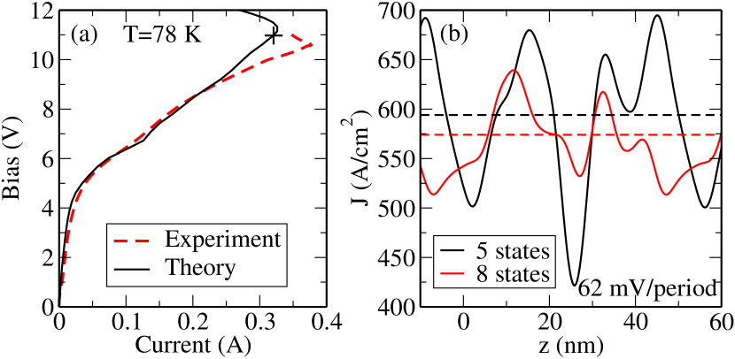
Figure 1: (a) Current-voltage characteristic for the THz-QCL of ref. KumarAPL2004 . In the calculations (full line) the bias was taken as 177 times the voltage drop per period and the area as $A=54\cdot 10^{-5}\textrm{cm}^{2}$. The cross marks the operation point at a bias drop of 62 mV per period. The experimental data (dashed line) are by courtesy of S. Kumar. (b) Spatially resolved current density from Eq. (3) for a calculation with 5 and 8 Wannier states per period, respectively (full lines). The dashed lines give the result from Eq. (2) for comparison.

In the upper panel of Fig. 2 the energetically resolved current density from Eq. (6) is displayed. At each energy one observes a current flow in $z$ direction due to the presence of nondiagonal elements in $G_{\beta\alpha}^{<}({\bf k},E)$. In order to satisfy the continuity of current, scattering transitions transfer particles between different energies, where the coherent evolution of the current continues. In addition, there are also elastic scattering events, where the current continues at the same energy, but with a different parallel momentum ${\bf k}$, which are visible in corresponding ${\bf k}$-resolved plots.

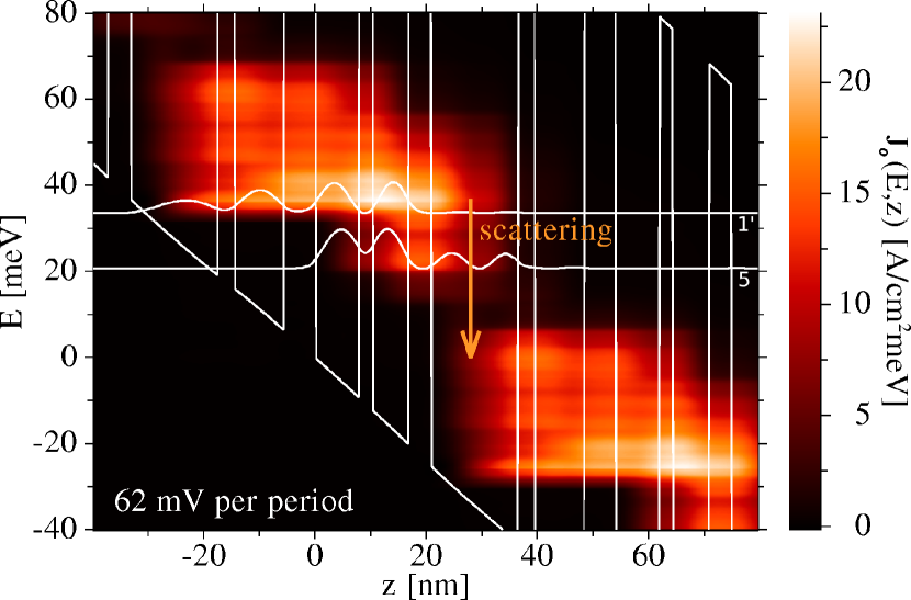
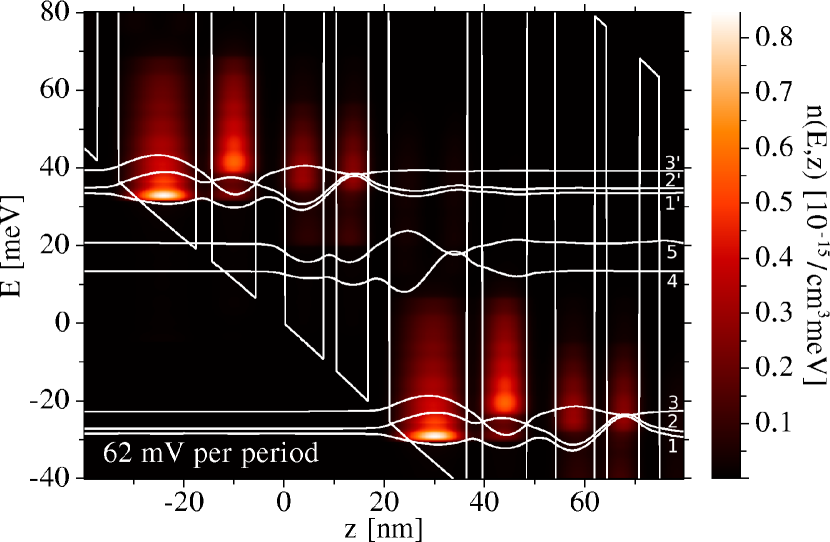
Figure 2: Upper panel panel: Spatially and energetically resolved current density evaluated by Eq. (6). The WS states $\varphi_{\alpha}^{2}(z)$ corresponding to the upper (1’) and lower (5) laser level are depicted for orientation. The vertical array marks a representative scattering transitions. Lower panel: Spatially and energetically resolved particle density evaluated by Eq. (7). The lowest five WS states $\varphi_{\alpha}(z)$ are displayed.

For comparison the energetically resolved particle density (see also KubisJCE2007 )

$$n(E,z)=\frac{2}{A}\sum_{\alpha\beta{\bf k}}\frac{1}{2\pi{\rm i}}G_{\beta\alpha}^{<}({\bf k},E)\varphi_{\alpha}^{*}(z)\varphi_{\beta}(z)$$ (7)

is shown in the lower panel of Fig. 2. It is intriguing to see, that neither the density nor the current profile follow the spatial profile of the WS-states. Furthermore note, that the states 1 and 2 resemble the binding and anti-binding combination of two more localized states.

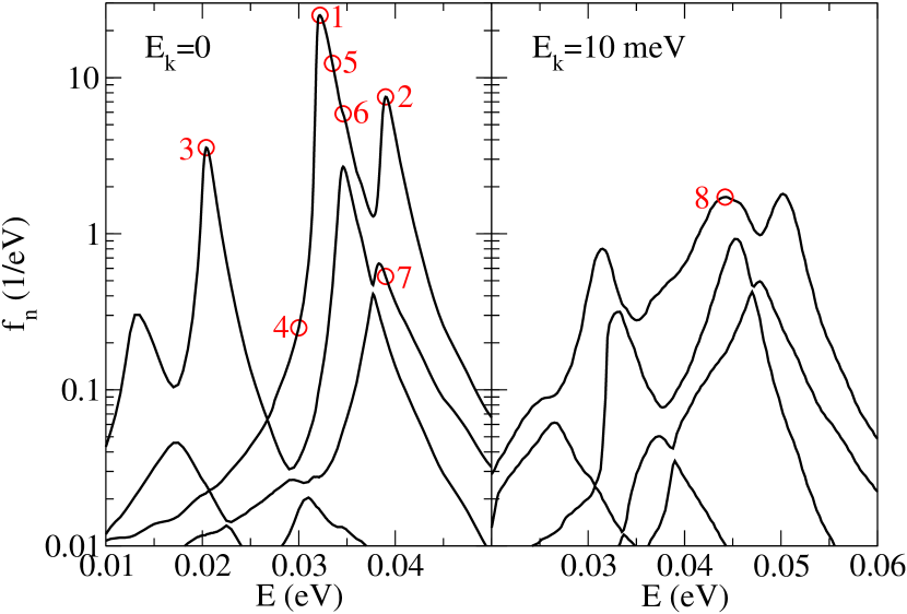
Figure 3: Eigenvalues of the matrix $G_{\beta\alpha}^{<}({\bf k},E)/(2\pi{\rm i})$ as a function of energy for two different values of ${\bf k}$. The states corresponding to the eigenvalues denoted by circles are displayed in Fig. 4.

In Fig. 3 the eigenvalues of $G_{\beta\alpha}^{<}({\bf k},E)/(2\pi{\rm i})$ are displayed as a function of energy. One can identify distinct peaks indicating the presence of broadened quasiparticle states. These can be attributed to specific branches in the eigenvalue spectrum, which however mix with each other at crossing points. The essential structure for ${\bf k}=0$ is repeated for finite k-values with a shift in energy by $E_{k}=\hbar^{2}k^{2}/2m$. For $E_{k}=10$ meV the width of the peaks is larger as more scattering states are present than for $E_{k}=0$ meV.

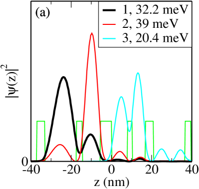
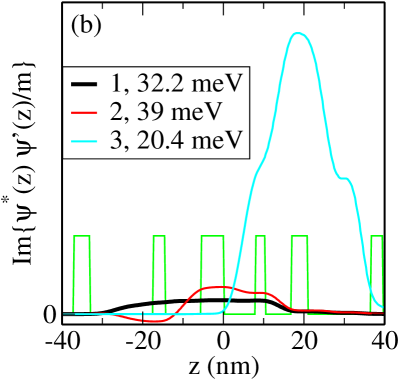
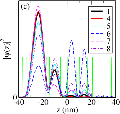
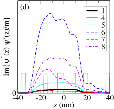
Figure 4: Wave functions $\Psi_{n{\bf k}}(E,z)$ which diagonalize $G_{\beta\alpha}^{<}({\bf k},E)/(2\pi{\rm i})$ for different energies and ${\bf k}$ corresponding to the eigenvalues denoted by the circles in Fig. 3.

In Fig. 4(a,b) the wave functions corresponding to the three largest eigenvalue peaks are shown. They describe the spatial structure of both the electron density and current displayed in Fig. 2. Thus they give a better description of the ongoing behavior than Wannier or Wannier-Stark states. In many cases these states are essentially unchanged if one follows a single branch of eigenvalues in Fig. 3. E.g., the states 1 and 4 differ only very slightly, see Fig. 4(c,d). However a strong energy dependence can occur due to mixing effects if different branches of eigenvalues come close to each other or even cross. This can be seen in the sequence for states 5, 6, and 7. The states for finite ${\bf k}$ are related to the corresponding states at ${\bf k}=0$ at the lower energy $E-E_{k}$. E.g., state 8 corresponds to states 5,6 (which are about 10 meV lower in energy $E$), albeit the mixing between different branches makes a detailed comparison difficult.

IV Density-matrix equations

Now we want to study the relation between the different approaches. In the NEGF approach, the results are determined by the lesser Greens function. For the stationary state, where

$$G^{<}(t,t^{\prime})=\int\frac{{\rm d}E}{2\pi}G^{<}(E){\rm e}^{-{\rm i}(t-t^{\prime})E/\hbar}\,,$$

Eq. (5.4) of Ref. HaugJauhoBook1996 provides us with

$$\begin{split}&\sum_{\gamma}G^{<}_{\alpha\gamma}(E,{\bf k})H^{0}_{\gamma\beta}({\bf k})-H^{0}_{\alpha\gamma}({\bf k})G^{<}_{\gamma\beta}(E,{\bf k})\\ &=\sum_{\gamma}\Big{[}\Sigma^{\rm ret}_{\alpha\gamma}(E,{\bf k})G^{<}_{\gamma\beta}(E,{\bf k})-G^{\rm ret}_{\alpha\gamma}(E,{\bf k})\Sigma^{<}_{\gamma\beta}(E,{\bf k})\\ &+\Sigma^{<}_{\alpha\gamma}(E,{\bf k})G^{\rm adv}_{\gamma\beta}(E,{\bf k})-G^{<}_{\alpha\gamma}(E,{\bf k})\Sigma^{\rm adv}_{\gamma\beta}(E,{\bf k})\Big{]}\end{split}$$ (8)

The self-energies are evaluated in the self-consistent Born-approximation providing

$$\begin{split}\Sigma^{<}_{\alpha\beta}&(E,{\bf k})=\sum_{\gamma\delta{\bf q}}V_{\alpha\gamma}({\bf q})V_{\delta\beta}(-{\bf q})\\ \times&\big{[}n_{\bf q}G^{<}_{\gamma\delta}(E-\hbar\omega_{\bf q},{\bf k}-{\bf q})\\ &+(n_{-{\bf q}}+1)G^{<}_{\gamma\delta}(E+\hbar\omega_{-{\bf q}},{\bf k}-{\bf q})\big{]}\\ \Sigma^{\rm ret/adv}_{\alpha\beta}&(E,{\bf k})=\sum_{\gamma\delta{\bf q}}V_{\alpha\gamma}({\bf q})V_{\delta\beta}(-{\bf q})\\ \times&\big{[}(n_{\bf q}+1)G^{\rm ret/adv}_{\gamma\delta}(E-\hbar\omega_{\bf q},{\bf k}-{\bf q})\\ &+n_{-{\bf q}}G^{\rm ret/adv}_{\gamma\delta}(E+\hbar\omega_{-{\bf q}},{\bf k}-{\bf q})\big{]}\end{split}$$ (9)

For illustrative purpose only phonon scattering with a single lateral mode ${\bf q}$ is taken into account here and the nondegenerate case is considered (otherwise additional terms with $G^{<}$ appear in $\Sigma^{\rm adv/ret}$). However, neither of these simplifications was performed in the numerical examples discussed above.

Neglecting any broadening effects, the full Greens functions can be approximated by the bare Greens functions

$$\begin{split}G^{\rm ret/adv}_{\alpha\beta}(E,{\bf k})\approx&\delta_{\alpha\beta}\frac{1}{E-E_{\beta}({\bf k})\pm{\rm i}0^{+}}\\ G^{<}_{\alpha\beta}(E,{\bf k})\approx&2\pi{\rm i}\rho_{\alpha\beta}\delta(E-E_{\alpha\beta}({\bf k}))\end{split}$$ (10)

A key issue is that we allow for a nondiagonal density matrix, which makes it difficult to address a specific energy $E_{\alpha\beta}({\bf k})$ to the respective $\delta$-function. A first guess is that $E_{\alpha\beta}({\bf k})$ is somehow related to $E_{\alpha}({\bf k})$ and/or $E_{\beta}({\bf k})$.

Now Eq. (9) is inserted into Eq. (8) and subsequently, the approximations (10) are inserted in the right-hand side. Integrating over $E$ and dividing by $2\pi{\rm i}$, provides

$$\begin{split}&\sum_{\gamma}\rho_{\alpha\gamma}({\bf k})H^{0}_{\gamma\beta}({\bf k})-H^{0}_{\alpha\gamma}({\bf k})\rho_{\gamma\beta}({\bf k})\\ &=\sum_{\gamma\delta{\bf q}}\Big{[}\frac{n_{-{\bf q}}V_{\alpha\delta}({\bf q})V_{\delta\gamma}(-{\bf q})\rho_{\gamma\beta}({\bf k})}{E_{\gamma\beta}({\bf k})-E_{\delta}({\bf k}-{\bf q})+\hbar\omega_{-{\bf q}}+{\rm i}0^{+}}\\ &\quad-\frac{n_{\bf q}V_{\alpha\gamma}({\bf q})\rho_{\gamma\delta}({\bf k}-{\bf q})V_{\delta\beta}(-{\bf q})}{E_{\gamma\delta}({\bf k}-{\bf q})-E_{\alpha}({\bf k})+\hbar\omega_{\bf q}+{\rm i}0^{+}}\\ &\quad+\frac{n_{\bf q}V_{\alpha\delta}({\bf q})\rho_{\delta\gamma}({\bf k}-{\bf q})V_{\gamma\beta}(-{\bf q})}{E_{\delta\gamma}({\bf k}-{\bf q})-E_{\beta}({\bf k})+\hbar\omega_{\bf q}-{\rm i}0^{+}}\\ &\quad-\frac{n_{-{\bf q}}\rho_{\alpha\gamma}({\bf k})V_{\gamma\delta}({\bf q})V_{\delta\beta}(-{\bf q})}{E_{\alpha\gamma}({\bf k})-E_{\delta}({\bf k}-{\bf q})+\hbar\omega_{-{\bf q}}-{\rm i}0^{+}}\Big{]}\\ &+\textrm{terms with }n_{\bf q}\to n_{-{\bf q}}+1\textrm{ and }\hbar\omega_{\bf q}\to-\hbar\omega_{-{\bf q}}\end{split}$$ (11)

Setting $E_{\gamma\beta}({\bf k})=E_{\gamma}({\bf k})$, $E_{\gamma\delta}({\bf k}-{\bf q})=E_{\gamma}({\bf k}-{\bf q})$, $E_{\delta\gamma}({\bf k}-{\bf q})=E_{\gamma}({\bf k}-{\bf q})$, and $E_{\alpha\gamma}({\bf k})=E_{\gamma}({\bf k})$ in the subsequent lines on the right-hand side, one obtains precisely the density-matrix kinetics of Sec IID of IottiPRB2005 in the so called complete collision limit. In this kinetics, the left-hand side has the additional term ${\rm i}\hbar\tfrac{{\rm d}\rho_{\alpha\beta}({\bf k})}{{\rm d}t}$, which however vanishes in the stationary case considered here.

In the density matrix equations, the choice of $E_{\alpha\beta}({\bf k})$, which accompanies the density matrix $\rho_{\alpha\beta}({\bf k})$ on the right-hand side, can be related to the way, the Markov limit is performed. Here different choices have been suggestedRossiPreprint2007 ; PedersenPRB2007 , which is an issue of ongoing debate. However, as shown below, the nondiagonal density matrices are small unless $|E_{\beta}({\bf k})-E_{\alpha}({\bf k})|\lesssim\Gamma$. If the properties of the system are constant on this energy scale, e.g., the temperature is larger than $\Gamma/k_{B}$, the specific choice of $E_{\alpha\beta}({\bf k})$ within the energy interval $[E_{\beta}({\bf k}),E_{\alpha}({\bf k})]$ is not of central relevance. Thus, the results for different choices should not differ dramatically as observed in PedersenPRB2007 . In the opposite case of small temperature ($<\Gamma/k_{B}$), broadening effects become of importance, which renders the density matrix approach questionable anyway.

V Hopping model

The ambiguity of choosing $E_{\alpha\beta}({\bf k})$ vanishes, if we assume that the diagonal density matrices $\rho_{\beta\beta}({\bf k})=f_{\beta}({\bf k})$ dominate the scattering terms which constitute the right-hand side of Eq. (11). This makes particular sense, if the states are chosen as the eigenstates of $\hat{H}^{0}$. For $\alpha=\beta$ we find

$$\begin{split}0=&-2\pi{\rm i}\sum_{\delta{\bf q}}n_{-{\bf q}}|V_{\alpha\delta}({\bf q})|^{2}\\ &\quad\times\delta(E_{\alpha}({\bf k})-E_{\delta}({\bf k}-{\bf q})+\hbar\omega_{-{\bf q}})f_{\alpha}({\bf k})\\ &+2\pi{\rm i}\sum_{\gamma{\bf q}}n_{\bf q}|V_{\alpha\gamma}({\bf q})|^{2}\\ &\quad\times\delta(E_{\gamma}({\bf k}-{\bf q})-E_{\alpha}({\bf k})+\hbar\omega_{\bf q})f_{\gamma}({\bf k}-{\bf q})\\ +&\textrm{terms with }n_{\bf q}\to n_{-{\bf q}}+1\textrm{ and }\hbar\omega_{\bf q}\to-\hbar\omega_{-{\bf q}}\end{split}$$ (12)

This is just the difference of out-scattering and in-scattering transition rates for the state $(\alpha,{\bf k})$, where the scattering rates are evaluated by Fermi’s golden rule. This defines the hopping model TsuPRB1975 which has been frequently applied to QCLs IottiPRL2001 ; CallebautAPL2004 ; BonnoJAP2005 ; JirauschekJAP2007 ; GaoAPL2007 . It is usually solved by the Monte Carlo technique and provides the stationary occupations $f_{\alpha}({\bf k})$.

For $\alpha\neq\beta$ the left-hand side of Eq. (11) provides the term $[E_{\beta}({\bf k})-E_{\alpha}({\bf k})]\rho_{\alpha\beta}$ in the eigenstate basis. Again the right-hand side has the magnitude of $\Gamma\times{\cal O}\{f_{\alpha}\}$, where $\Gamma/\hbar$ is the magnitude of the scattering rate for a single level. Therefore does the assumption, that the diagonal elements dominate the density matrix, become questionable if a pair of levels satisfies $|E_{\beta}({\bf k})-E_{\alpha}({\bf k})|\lesssim\Gamma$ which is typical for level crossings, see also the discussion in CallebautJAP2005 .

The evaluation of the current is a subtle issue, as the current is entirely contained in the nondiagonal density matrices as discussed above. Now Eq. (2) gives in the eigenstate basis:

$$J=-\frac{e}{\hbar V}\sum_{\alpha\neq\beta,{\bf k}}z_{\beta\alpha}\Im\left\{[E_{\beta}({\bf k})-E_{\alpha}({\bf k})]\rho_{\alpha\beta}\right\}$$ (13)

where the antisymmetry of $W_{\alpha\beta}$ was used. Now $[E_{\beta}({\bf k})-E_{\alpha}({\bf k})]\rho_{\alpha\beta}$ is precisely the left-hand side of Eq. (11) and restricting to the dominating diagonal density matrices on the right-hand side we obtain

$$\begin{split}J=&\frac{2\pi e}{\hbar V}\sum_{\alpha\neq\beta,{\bf k}}z_{\beta\alpha}\\ \times&\Big{[}\sum_{\delta{\bf q}}n_{-{\bf q}}V_{\alpha\delta}({\bf q})V_{\delta\beta}(-{\bf q})\\ &\times\delta(E_{\beta}({\bf k})-E_{\delta}({\bf k}-{\bf q})+\hbar\omega_{-{\bf q}})f_{\beta}({\bf k})\\ &-\sum_{\gamma{\bf q}}n_{\bf q}V_{\alpha\gamma}({\bf q})V_{\gamma\beta}(-{\bf q})\\ &\times\delta(E_{\gamma}({\bf k}-{\bf q})-E_{\alpha}({\bf k})+\hbar\omega_{\bf q})f_{\gamma}({\bf k}-{\bf q})\Big{]}\\ +&\textrm{terms with }n_{\bf q}\to n_{-{\bf q}}+1\textrm{ and }\hbar\omega_{\bf q}\to-\hbar\omega_{-{\bf q}}\end{split}$$ (14)

where we used that the lower two lines are the complex anti-conjugate of the upper two lines in the right-hand side of Eq. (11) after exchanging the indices $\alpha$ and $\beta$. Now the completeness of the states $\varphi_{\alpha}(z)$ in the $z$-part of the Hilbert space provides the relation

$$\sum_{\alpha\neq\beta}z_{\beta\alpha}V_{\alpha\delta}({\bf q})=\sum_{\beta}\left[\langle\beta|\hat{z}V(z,{\bf q})|\delta\rangle-z_{\beta\beta}V_{\beta\delta}({\bf q})\right]$$

to be used in the first summand of Eq. (14). In addition the running index $\delta$ is replaced by $\alpha$. Correspondingly,

$$\sum_{\alpha\neq\beta}V_{\gamma\beta}(-{\bf q})z_{\beta\alpha}=\\ \sum_{\alpha}\left[\langle\gamma|\hat{z}V(z,-{\bf q})|\alpha\rangle-z_{\alpha\alpha}V_{\gamma\alpha}(-{\bf q})\right]$$

is used in the second summand with the replacements $\gamma\to\beta$ as well as ${\bf k}-{\bf q}\to{\bf k}$ and ${\bf q}\to-{\bf q}$. These operations result in

$$\begin{split}J=&\frac{2\pi e}{\hbar V}\sum_{\alpha\beta,{\bf k},{\bf q}}n_{-{\bf q}}|V_{\beta\alpha}({\bf q})|^{2}(z_{\alpha\alpha}-z_{\beta\beta})\\ &\times\delta(E_{\beta}({\bf k})-E_{\gamma}({\bf k}-{\bf q})+\hbar\omega_{-{\bf q}})f_{\beta}({\bf k})\\ +&\textrm{terms with }n_{\bf q}\to n_{-{\bf q}}+1\textrm{ and }\hbar\omega_{\bf q}\to-\hbar\omega_{-{\bf q}}\end{split}$$ (15)

which is the standard expression for hopping currents. It can be interpreted as the sum of scattering transitions from $\beta$ to $\alpha$, which change the mean location of the electron from $z_{\beta\beta}$ to $z_{\alpha\alpha}$. This is however not the underlying physics, as scattering does not directly change the particle position. In contrast the entire current is carried by the polarizations $\rho_{\alpha\beta}$ and Eq. (15) is nothing but an approximation for these coherences.

VI Conclusion

The transport in QCLs and similar structure such as superlattice is entirely due to coherences, i.e. nondiagonal elements in the density matrix $\rho_{\alpha\beta}({\bf k})$ if a set of real basis functions is chosen. The use of NEGF allows for a spatially and energetically resolved visualization of these coherent transport properties. Neglecting the energetic broadening of the states, the density matrix equations can be derived from NEGF theory. However, the energetic location of the nondiagonal elements is only poorly defined in this reduction scheme. If the level differences are larger than the scattering induced broadening $\Gamma$, the nondiagonal elements of the density matrix are small and can be approximated by differences in level occupation. In this way the frequently used hopping model for the current appears. This model suggests the interpretation that the spatial position of the particles is directly changed by the individual scattering processes. However one has to keep in mind, that conventional scattering processes do not change the position of carrier, but only induce coherences which subsequently drive the current.

- (1) J. Faist, F. Capasso, D. L. Sivco, C. Sirtori, A. L. Hutchinson, and A. Y. Cho, Science 264, 553 (1994).
- (2) R. Köhler, A. Tredicucci, F. Beltram, H. E. Beere, E. H. Linfield, A. G. Davies, D. A. Ritchie, R. C. Iotti, and F. Rossi, Nature 417, 156 (2002).
- (3) M. Lee and M. C. Wanke, Science 316(5821), 64 (2007).
- (4) J. Devenson, R. Teissier, O. Cathabard, and A. N. Baranov, Appl. Phys. Lett. 90, 111118 (2007).
- (5) G. Scalari, C. Walther, J. Faist, H. Beere, and D. Ritchie, Appl. Phys. Lett. 88, 141102 (2006).
- (6) F. Capasso, J. Faist, and C. Sirtori, J. Math. Phys. 37, 4775 (1996).
- (7) P. Harrison, Appl. Phys. Lett. 75, 2800 (1999).
- (8) D. Indjin, P. Harrison, R. W. Kelsall, and Z. Ikonic, J. Appl. Phys. 91, 9019 (2002).
- (9) R. C. Iotti and F. Rossi, Phys. Rev. Lett. 87, 146603 (2001).
- (10) H. Callebaut, S. Kumar, B. S. Williams, Q. Hu, and J. L. Reno, Appl. Phys. Lett. 84, 645 (2004).
- (11) O. Bonno, J. Thobel, and F. Dessenne, J. Appl. Phys. 97, 043702 (2005).
- (12) C. Jirauschek, G. Scarpa, P. Lugli, M. S. Vitiello, and G. Scamarcio, J. Appl. Phys. 101, 086109 (2007).
- (13) X. Gao, D. Botez, and I. Knezevic, Journal of Applied Physics 101, 063101 (2007).
- (14) R. Tsu and G. Döhler, Phys. Rev. B 12, 680 (1975).
- (15) D. Calecki, J. F. Palmier, and A. Chomette, J. Phys. C: Solid State Phys. 17, 5017 (1984).
- (16) C. Sirtori, F. Capasso, J. Faist, A. Hutchinson, D. L. Sivco, and A. Y. Cho, IEEE J. Quantum Electron. 34, 1772 (1998).
- (17) H. Callebaut and Q. Hu, J. Appl. Phys. 98, 104505 (2005).
- (18) S. C. Lee and A. Wacker, Phys. Rev. B 66, 245314 (2002).
- (19) S. C. Lee, F. Banit, M. Woerner, and A. Wacker, Phys. Rev. B 73, 245320 (2006).
- (20) R. C. Iotti, E. Ciancio, and F. Rossi, Phys. Rev. B 72, 125347 (2005).
- (21) A. Wacker, Phys. Rep. 357, 1 (2002).
- (22) H. Haug and A. P. Jauho, Quantum Kinetics in Transport and Optics of Semiconductors (Springer, Berlin, 1996).
- (23) S. Kumar, B. S. Williams, S. Kohen, Q. Hu, and J. L. Reno, Appl. Phys. Lett. 84, 2494 (2004).
- (24) F. Banit, S. C. Lee, A. Knorr, and A. Wacker, Appl. Phys. Lett. 86, 41108 (2005).
- (25) T. Kubis and P. Vogl, J. Comput. Electron. 6, 183 (2007).
- (26) F. Rossi, Quantum Fermi’s golden rule, arXiv:quant-ph/0702233v1.
- (27) J. N. Pedersen, B. Lassen, A. Wacker, and M. H. Hettler, Phys. Rev. B 75, 235314 (2007).