Equation of State for Macromolecules of Variable Flexibility in Good Solvents: A Comparison of Techniques for Monte Carlo Simulations of Lattice Models

Abstract

The osmotic equation of state for the athermal bond fluctuation model on the simple cubic lattice is obtained from extensive Monte Carlo simulations. For short macromolecules (chain length N=20) we study the influence of various choices for the chain stiffness on the equation of state. Three techniques are applied and compared in order to critically assess their efficiency and accuracy: the “repulsive wall” method, the thermodynamic integration method (which rests on the feasibility of simulations in the grand canonical ensemble), and the recently advocated sedimentation equilibrium method, which records the density profile in an external (e.g. gravitation-like) field and infers, via a local density approximation, the equation of state from the hydrostatic equilibrium condition. We confirm the conclusion that the latter technique is far more efficient than the repulsive wall method, but we find that the thermodynamic integration method is similarly efficient as the sedimentation equilibrium method. For very stiff chains the onset of nematic order enforces the formation of an isotropic–nematic interface in the sedimentation equilibrium method leading to strong rounding effects and deviations from the true equation of state in the transition regime.

I Introduction

Understanding the equation of state of macromolecules in solution has been a longstanding problem of polymer science, which is both important as a fundamental problem in the statistical mechanics of soft matter Flory ; deGennes ; Cloizeaux ; Grosberg ; Binder ; Schafer ; Rubinstein and relevant for various applications of polymers. The interplay of excluded volume effects deGennes ; Cloizeaux ; Grosberg ; Schafer , solvent quality and variable chain stiffness Grosberg ; KhoSem already is very difficult to describe for macromolecules in very dilute solution Seeeg , withstanding an analytic solution and making the application of computer simulation methods Binder ; Kotelyanskii necessary. The experimental situation on measurements of the equation of state of polymer solutions is addressed in chapter $5$ of Ref. Cloizeaux, and chapter $3$ of Ref. Strobl, . Considering semidilute and concentrated solutions, the enthalpic and/or entropic interactions among the polymer chains create nontrivial correlations in the structure of the solutions involving many chains, and phase transitions such as phase separation under bad solvent conditions into a dilute polymer solution and a concentrated one may occur Flory ; deGennes ; Widom ; CBGC ; Binder2 . Alternatively, under good solvent conditions one may observe for semiflexible or for stiff chains a transition from an isotropic to a nematic solution when the polymer concentration increases Flory2 ; Baumgartner ; Weber ; Strey ; Vega . Of particular interest is the situation when nematic ordering and the tendency to phase separation under bad solvent conditions compete Khokhlov . Preliminary computer simulation studies of a corresponding model LCpaper1 ; LCpaper2 gave only rather rough information on the phase behavior, and it was concluded that the accuracy with which the osmotic equation of state could be determined needs to be improved.

Thus, there are many reasons why establishing methods that allow the reliable estimation of the equation of state for various coarse-grained lattice models for polymers is of interest. While in an off-lattice model the estimation of the pressure tensor from the virial theorem in principle is straightforward Allen , it often is not possible to study very large systems with the desirable accuracy Binder , and hence simulations of lattice models still have their place Binder ; Kotelyanskii . However, for lattice models different techniques to calculate the osmotic pressure of polymers in solution must be sought in order to derive their equation of state. The standard method, particularly valuable for dilute solutions and/or not too large chain lengths, calculates the chemical potential from the insertion probability of a test chain Bell ; latt1eos and the osmotic pressure then follows from standard thermodynamic integration Binder ; Allen ; Frenkel ; Landau . As is well known, insertion of a polymer chain into a volume containing already other chains is very difficult due to very small acceptance probabilities, and hence requires advanced Monte Carlo methods Frenkel ; Siepmann ; MuellerPaul to be practically feasible.

As an alternative method Dickman rep_wall1 ; rep_wall2 proposed the repulsive wall thermodynamic integration (RWTI) method, which remains applicable also for very dense systems since it works in the canonic (${\cal N}VT$) ensemble, where the number of chains $\cal N$ in the box remains fixed. However, this method requires substantial simulation effort, since for each state point in the bulk several simulation runs with increasing wall–monomer repulsion and subsequent thermodynamic integration need to be performed. Moreover the RWTI method may suffer from important finite size effects PressPaper .

More recently, it was proposed Hansen to extract the osmotic equation of state from Monte Carlo simulations where the equilibrium monomer and center-of-mass concentration profiles of lattice polymers in a gravitation-like potential are computed. From these concentration profiles, the equation of state can be inferred if a local density approximation like in hydrostatic equilibrium is invoked. This method has been broadly applied to study the sedimentation equilibrium of colloidal dispersions containing spherical BibenHansen , rod-like Dijkstra04 or disk-like DijkstraHansen particles. More recently, successful applications to colloid-polymer mixtures HansenJPCM and solutions of block copolymers HansenMolPhy or binary polymer solutions HansenJPCB have been made as well.

Despite these successes, this “sedimentation equilibrium” (SE) method also may have drawbacks, when other large length scales appear in the system, that compete with the characteristic “sedimentation length”. This length that scales inversely with the “gravitational constant” characterizing the gravitation-like potential and hence can be made arbitrarily large Hansen , but the linear dimension of the simulated system in the $z$-direction in which this gravitation-like force acts must then be huge, also. A well-known case, where even the real gravitation potential on earth substantially disturbs the equation of state is a fluid very close to the gas-liquid critical point HohenBarm , since there the correlation length of density fluctuations diverges, and critical fluctuations undisturbed by gravity can occur in the $x,y$-directions perpendicular to the gravitational force only HohenBarm . Other cases, apart from critical points of second-order transitions, where large length scales arise that are potentially disturbed by the gravitation-like potential are associated with the formation of thick wetting layers at walls, for instance.

While Addison at al. Hansen did test the SE method against the RWTI method for a few cases varying the solvent quality from good solvents to theta solvents, finding good agreement, they considered only fully flexible chains. Thus, we take up this problem but rather consider semiflexible chains as well: the possible occurrence of nematically ordered wetting layers at the wall where the density is largest Dijkstra03 or even the occurrence of the isotropic to nematic transition in the bulk solution of the semiflexible or stiff polymers may complicate matters. The aim of the present work is to carefully test the SE method against both the RWTI method and the standard thermodynamic integration method in the grand canonical $\mu VT$ ensemble (TI$\mu VT$ method, $\mu$ denoting the chemical potential), and to assess by detailed comparisons both the efficiency and the accuracy of these methods. As has been explained above, there is need for accurate simulation methods for the computation of the equation of state of polymer solutions in the context of various interesting problems.

The plan for the remainder of this paper is as follows. In Sec. II we briefly review the theoretical basis for the RWTI, TI$\mu VT$ and SE methods, while Sec. III describes the simulated model and mentions the types of Monte Carlo moves used. Sec. IV presents comparisons of the three methods for fully flexible chains over a wide range of densities, while Sec. V presents our results for variable chain stiffness. Sec. VI contains our conclusions and gives an outlook to future work.

II Methods to calculate the osmotic pressure for lattice models of polymer solutions

II.1 Thermodynamic integration in the grand canonical ensemble (TI$\mu VT$ method)

We consider a system of chains of length $N$ in a simulation box of volume $V$ with periodic boundary conditions (typically the box has a cubic shape, $V=L^{3}$, $L$ being the linear dimension) at given temperature $T$ and chemical potential $\mu$ of the chains. The density of polymer chains in the system, $\rho={\cal N}/V$, with ${\cal N}$ the average number of chains contained in the simulation box then is an output of the simulation.

Utilizing the standard relations in the canonical ensemble, $\mu=(\partial(F/V)/\partial\rho)_{T,V}$ and $p=-(\partial F/\partial V)_{T,{\cal N}}$, where $F$ is the free energy of the system and $p$ the pressure, one easily derives that

$$p=\rho\mu-\int\limits^{\rho}_{0}\mu(\rho^{\prime})d\rho^{\prime}+const,$$ (1)

where the integration constant in Eq. (1) can be fixed by reference to the low density limit, where the system behaves like an ideal gas of chains,

$$pV={\cal N}k_{B}T,\quad\pi\equiv p/k_{B}T=\rho.$$ (2)

Denoting then the chemical potential of the ideal gas of chains as $\mu_{id}$, and defining $\mu^{ex}=\mu-\mu_{id}$ the excess chemical potential per chain, Eqs. (1),(2) imply Bell

$$\pi=\rho(1+\mu^{ex})-\int\limits_{0}^{\rho}\mu^{ex}(\rho^{\prime})d\rho^{\prime}$$ (3)

In practice the integral in Eq. (3) is discretized, so that the reduced osmotic pressure $\pi_{i}$ at chain density $\rho_{i}$ is obtained from the recursion relation

$$\pi_{i}\approx\pi_{i-1}+(1+\mu_{i}^{ex})\rho_{i}-(1+\mu_{i-1}^{ex})\rho_{i-1}-(\mu^{ex}_{i}+\mu^{ex}_{i-1})(\rho_{i}-\rho_{i-1})/2.$$ (4)

The disadvantages of the method are clearly obvious from Eq. (4): a large number of state points $\{\mu_{i},T,V\}$ needs to be studied with small differences between $\mu_{i}$ and $\mu_{i-1}$ and hence $\rho_{i}$ and $\rho_{i-1}$, so that the discretization error going from Eq. (3) to Eq. (4) is negligible; and an efficient grand canonical simulation method is needed, so $\rho_{i}$ is sampled with sufficient accuracy. For not too long chains and not too high densities, however, the method is indeed practically useful, and since periodic boundary conditions are used, the system for large $V$ always is homogeneous, and the analysis is not hampered by any interfacial effects, which are present inevitably in the other techniques described below due to their explicit use of walls.

II.2 The repulsive wall thermodynamic integration (RWTI) method

This method can be implemented both in the grand canonical $\mu VT$ ensemble and in the canonical ${\cal N}VT$ ensemble. While the latter choice has the advantage that no chain insertions are necessary and hence the method also works for long chains and at high densities, it suffers from rather large finite size effects PressPaper . We have used here both the canonical and the grand canonical version of the method.

One considers now a box of linear dimensions $L\times L\times H$, with periodic boundary conditions in $x$ and $y$ directions only, while a hard wall is placed both at $z=0$ and $z=H$. Moreover, one introduces a repulsive potential of strength $\varepsilon_{wall}$ which acts in the first layer adjacent to $z=0$ and in the last layer available to the monomers, $z=H$. As discussed in rep_wall1 ; rep_wall2 ; PressPaper , the osmotic pressure is then obtained from the fraction of sites, $\phi_{z}(\lambda)$, occupied by monomers in the layers adjacent to both walls, $z=0$ and $z=H$,

$$\pi=\int\limits_{0}^{1}\frac{d\lambda}{\lambda}\left(\frac{\phi_{z=0}(\lambda)+\phi_{z=H}(\lambda)}{2}\right),\quad\lambda\equiv\exp(-\varepsilon_{wall}/k_{B}T).$$ (5)

Again the integration in Eq. (5) is discretized, and 20 different values of $\lambda$ turned out to be sufficient to obtain reliable results.

II.3 The sedimentation equilibrium (SE) method

This method utilizes the canonical ensemble ${\cal N}VT$, and one also considers a box of linear dimensions $L\times L\times H$ with periodic boundary conditions in $x$ and $y$ directions only, while again hard walls are used in $z$-direction at $z=0$ and at $z=H$. An external potential is applied not at the walls but everywhere in the system Hansen

$$U_{\rm external}(z)=-mgz=-\frac{\displaystyle k_{B}T}{\displaystyle a}\lambda_{g}z.$$ (6)

Here $m$ is the mass of a monomer, $g$ is the acceleration due to the gravity-like potential, $a$ is the lattice spacing, and $\lambda_{g}$ is a dimensionless constant that characterizes the strength of this gravitational potential, $\lambda_{g}=amg/k_{B}T$. It is also useful to introduce characteristic gravitational lengths $\xi_{m},\xi_{cm}$

$$\xi_{m}=a/\lambda_{g},\quad\xi_{cm}=\xi_{m}/N.$$ (7)

As shown by Addison et al. Hansen , for large $z$ the density profile of an ideal gas of monomers at the lattice would follow the standard barometric formula, $\rho_{m}(z)\propto\exp(-mgz/k_{B}T)=\exp(-z/\xi_{m})$, while for an ideal gas of polymer chains the density profile of monomer units $\rho_{m}(z)=N\rho(z)\propto\exp(-z/\xi_{cm})$.

While the variation of the density profile for large $z$, where the system is very dilute and the ideal gas behavior holds, hence is trivially known, and this knowledge is an important consistency check of the method, for smaller $z$ the density profile is nontrivial. But from this profile the osmotic equation of state can be estimated, when one invokes the local density approximation, such that the equation of hydrostatic equilibrium holds Hansen ; BibenHansen

$$\frac{\displaystyle dp(z)}{\displaystyle dz}=-Nmg\rho(z),$$ (8)

$p(z)$ being the local osmotic pressure at altitude $z$. Integration of Eq.(8) yields

$$\pi(z)=p(z)/k_{B}T=\xi^{-1}_{cm}\int\limits^{\infty}_{z}\rho(z^{\prime})dz^{\prime}.$$ (9)

Thus one can record both $\rho(z)$ (and the associated monomer profile $\rho_{m}(z)$) and $\pi(z)$ simultaneously, and eliminating $z$ from these relations one obtains the desired equation of state $\pi(\rho)$ (or $\pi(\rho_{m})$, respectively).

Noting that in the local density approximation we expect that the density distribution of the monomer units satisfies $\rho_{m}(z)=N\rho(z)$, we find from Eqs. (7), (9) that $\pi(z)$ can also be written as

$$\pi(z)=\xi^{-1}_{m}\int\limits^{\infty}_{z}\rho_{m}(z^{\prime})dz^{\prime}.$$ (10)

However, the validity of the local density approximation needs to be considered carefully. E.g., near the hard wall at $z=0$, $\rho_{m}(z)$ may exhibit strong oscillations (“layering”), and also $\rho(z)$ exhibits a nontrivial structure. Thus it is clear that the local density approximation breaks down near the hard wall at $z=0$, and in fact one should use Eqs. (9),(10) only for $z\geq R_{g}$, the gyration radius of the chains. Similarly, rapid density variations invalidating the local density approximation are also expected near an interface between coexisting phases (as it may occur for bad solvent conditions, for instance). In addition, one must require that on the scale of $\Delta z=R_{g}$ the change of the potential, Eq. (6), is negligibly small. This implies

$$\left|\Delta U_{\rm external}(\Delta z)/k_{B}T\right|=\lambda_{g}R_{g}/a=R_{g}/\xi_{m}\ll 1.$$ (11)

For flexible chains, $R_{g}$ scales like $\sqrt{N}$ in concentrated solutions, while for stiff chains we have $R_{g}\propto N$. This implies that for stiff chains considerably larger values of $\xi_{m}$ (and hence smaller values of $\lambda_{g}$) need to be chosen than for flexible ones. Of course, since one must accommodate in the simulation box the full density profile from a value appropriate for concentrated solutions near $z=0$ down to the dilute regime near $z=H$, a linear dimension $H\gg\xi_{m}$ is mandatory; otherwise, the distortion of the density profile due to this upper boundary at $z=H$ leads to systematic errors as well. Thus, the SE method requires a careful choice of simulation parameters to avoid such errors and ensure the desired very good accuracy, and the large size $H$ in $z$-direction to some extent will reduce the advantage, that the whole equation of state can be estimated from a single run.

Finally we note that the approach can be generalized to other forms of the external potential $U_{external}(z)$, different from a gravitation-like potential. E.g., if one uses

$$U^{\prime}_{\rm external}(z)=-\frac{\displaystyle k_{B}T}{\displaystyle a}\lambda^{\prime}_{g}z^{\kappa},$$ (12)

where $\kappa$ is an exponent different from one, the equation for the force balance at height $z$ {Eq. 8} gets modified as

$$\frac{\displaystyle dp(z)}{\displaystyle dz}=-(\lambda^{\prime}_{g}/a)\kappa\rho(z)z^{\kappa-1},$$ (13)

and hence

$$\pi(z)=(\xi^{\prime}_{m})^{-1}\int\limits^{\infty}_{z}\kappa{\tilde{z}}^{\kappa-1}\rho_{m}({\tilde{z}})d{\tilde{z}}.$$ (14)

Motivation for using different potentials can be experiments made in a centrifuge. The centrifugal force depends linearly on the distance from the center of rotation, so that $\kappa=2$ for this case. Although it is not clear at this point which choice for the exponent $\kappa$ is optimal, testing that the equation of state $\pi(\rho_{m})$ thus obtained does not depend on $\kappa$ is a nice consistency check.

III Model and Simulation Technique

We use the bond fluctuation model BFM on the simple cubic lattice, taking henceforth $a\equiv 1$ as our unit of length. Each effective monomeric unit is represented by an elementary cube of the lattice, blocking all 8 sites at the corners of this cube from further occupation, realizing thus the excluded volume interaction between the monomers. The bond vectors can be taken from the set $\left\{(\pm 2,0,0),(\pm 2,\pm 1,0),(\pm 2,\pm 1,\pm 1),(\pm 2,\pm 2,\pm 1),(\pm 3,0,0),(\pm 3,\pm 1,0)\right\}$, including also all permutations between these coordinates, – altogether 108 different bond vectors occur, which leads to 87 different angles between successive bonds. To model the chain stiffness, an intramolecular potential depending on the angle $\vartheta$ between two successive bond vectors along the chain is introduced (bending energy), and also an energy term depending on the bond length $b$ can be included Weber ,

$$U_{\rm bending}=U_{\vartheta}+U_{b}=-f\cos\vartheta(1+c\cos\vartheta)+\varepsilon_{0}\left(b-b_{0}\right)^{2}.$$ (15)

Both the stiffness parameter $f$ and $\varepsilon_{0}$ are measured in units of $k_{B}T$. Note that for the model with $f=2.68$, $\varepsilon_{0}=4$, $b_{0}=0.86$, $c=0.03$ the isotropic to nematic transition has been studied by extensive Monte Carlo simulations previously Weber , and in order to be able to compare the present results to previous work we have included this bond length energy term here again.

Note that variable solvent quality can be modeled by including also a square well potential between any pair of monomers,

$$U_{\rm SW}(r)=\begin{cases}-\varepsilon,&r\leq\sqrt{6}\\ 0,&r>\sqrt{6},\end{cases}$$ (16)

as done in Refs. CBGC, ; LCpaper1, . However, the present work will treat the case $\varepsilon=0$ only, our analysis of the phase behavior when both $f$ and $\varepsilon$ are nonzero is deferred to a later work.

For the runs in the ${\cal N}VT$ ensemble (for the RWTI and SE methods) we define two Monte Carlo steps (MCS) to involve one attempt to perform a local “random hopping” move per each monomer unit in the system BFM and one attempt of a slithering-snake move per chain. These are the standard moves for simulations using the bond fluctuation model Binder ; Binder3 in the canonical ensemble. The chain length used was $N=20$ throughout, while typical box sizes were $90\times 90\times 90$ and $60\times 60\times 180$ for the RWTI method and $80\times 80\times 250$ for the SE method, respectively. For the SE method, a typical system contained ${\cal N}=1000$ chains, and about $10^{7}$ MCS were needed to get a reasonably well equilibrated density profile. For the RWTI method, the number of chains in the box was varied from very small number up to about ${\cal N}=3000$. Again typically $10^{7}$ MCS per run were used, taking $10^{4}$ “measurements” in each run, with $10^{3}$ MCS between two successive measurements (it was checked that these $10^{4}$ configurations then were uncorrelated).

For the runs in the $\mu VT$ ensemble, one Monte Carlo step means one configurational bias move CBGC ; LCpaper1 ; Frenkel ; Siepmann plus additionally either one attempt to perform a local random hopping move of every effective monomer in the system or one attempt of a slithering-snake move per chain. For the TI$\mu VT$ method, about 50–60 different values of the chemical potential were used, and the box size was $90\times 90\times 90$. For each parameter combination $3\cdot 10^{5}$ MCS were taken. The maximum value of the number of chains reached was about ${\cal N}=2700$ (this corresponds to the polymer volume fraction of about $\phi=0.6$ in this simulation box). So the total number of MCS needed to record the equation of state is of the order of $2\cdot 10^{7}$ MCS (but note that 1 MCS needs an amount of CPU time which depends on the number of chains ${\cal N}$ in the system).

Since it is well known Binder ; Landau that in the ${\cal N}VT$ ensemble the equilibration of long wavelength density fluctuations is very slow, suffering from “hydrodynamic slowing down” Landau , it is useful to take special precautions that the density profiles in the RWTI are well equilibrated, in order to avoid uncontrolled errors. Therefore for each value of the repulsive wall parameter $\lambda$ {cf. Eq. (5)} we first equilibrated the system in the $\mu VT$ ensemble, choosing $\mu$ appropriately to reach the desired value of ${\cal N}$. Again $3\cdot 10^{5}$ steps were used for this grand canonical equilibration stage. Then the configurational bias moves were stopped, and the ${\cal N}VT$ run with the measurement of the number of monomers $N_{wall}(\lambda)$ adjacent to the walls began.

In the configurational bias moves, one needs to utilize a biased chain insertion method to let a polymer “grow” successively into the system. At each step all possible 108 bond vectors from the current effective monomer are examined, and a position for inserting the next monomeric unit along the chain is chosen, respecting the excluded volume condition, and using the Boltzmann weight calculated from the intramolecular energy, Eq. (15). The statistical weight of the generated polymer configuration hence is easily calculated recursively, and thus the bias can be accounted for in the acceptance probability for the move.

In our simulations, we have recorded standard single-chain characteristics such as the mean-square end-to-end distance $R_{e}$ and the mean-square gyration radius $R_{g}$ of the chains ($\vec{r}_{i}$ are positions of monomers, $\vec{r}_{CM}$ is the position of the center of mass),

$$R_{e}=\left<(\vec{r}_{N}-\vec{r}_{1})^{2}\right>^{1/2},\quad R_{g}=\left<\sum_{i=1}^{N}(\vec{r}_{i}-\vec{r}_{cm})^{2}/N\right>^{1/2},$$ (17)

from the runs in the $\mu VT$ ensemble. Note that these quantities depend on the polymer volume fraction $\phi=8{\cal N}Na^{3}/V$ in the system, or the average density of monomer units $\rho_{m}=\phi/8a^{3}$. The average $\left<\ldots\right>$ extends over all chains and all generated system configurations. In the SE method, where we have a density profile from a rather large density near $z=0$ to almost zero at $z=H$, we expect that the radii $R_{e},R_{g}$ will depend distinctly on the height $z_{CM}$ of the center of mass of a chain, and hence this information could only be obtained with substantially reduced statistical accuracy. In the RWTI method, one can estimate the radii as well if one restricts the averaging to chains with center of mass coordinate $\vec{r}_{CM}$ sufficiently remote from the walls.

IV Results for Fully Flexible Chains

We start by comparing results obtained from the RWTI method with results obtained from the thermodynamic integration in the grand canonical ensemble (Fig. 1). The agreement between the results of both methods actually is excellent (relative deviations are smaller than $10^{-2}$, and the statistical error for all data points obtained by both methods was also always less than 1%). Also the old data by Deutsch and Dickman rep_wall2 , which clearly are considerably less accurate, agree with the present calculation to within a few percent.

An essential consideration for the TI$\mu VT$ method is that the values of $\mu$ for which calculations are performed must be so closely spaced that the probability distributions $P_{\mu}(\rho_{m})$ at neighboring choices of $\mu$ overlap strongly. This condition has been carefully checked. Note, however, that the effort in CPU resources to generate the full equation of state $\pi(\phi)$ in Fig. 1 with the TI$\mu VT$ method is comparable to the effort for a single point on the equation of state in the RWTI method. Therefore we restrained our efforts to the accurate calculation of two state points with this method only.

Fig. 2 now compares the results obtained with the SE method with those of the TI$\mu VT$ method, and again we find perfect agreement. Note that the choice $\lambda_{g}=0.01$ implies a length $\xi_{m}=100$ {Eq. (7)}, while the gyration radius is $R_{g}\approx 6.4$ for $N=20$ and volume fractions in the range from $0.1<\phi<0.2$, which are relevant here. Thus the condition $R_{g}\ll\xi_{m}$ {Eq. (11)} is safely fulfilled, but nevertheless it is important to check that no visible systematic error of the SE method is present (to our knowledge, it is not known in which order of $R_{g}/\xi_{m}$ systematic corrections due to the gradient in density should be expected). As expected, we see some increase of the random statistical error with increasing $\phi$, but the absolute magnitude of this error always stays clearly below $10^{-3}$, and the relative error is between 1% and 2%.

Thus we confirm the conclusion of Addison et al. Hansen , for a different model than studied in their work, that the SE method can yield a reliable estimation of the equation of state. However, care has to be exerted that parameters such as the height $H$ of the simulation box and the strength of the external potential $\lambda_{g}$ are chosen appropriately, and also the statistical effort needs to be large enough. Figs. 3 and 4 contain examples of the problems that one encounters when these conditions are not met. E.g., when the potential is chosen too weak for the chosen size $H$ (and number of chains ${\cal N}$), so that the density profile (we plot here and below profiles of the polymer volume fraction $\phi$) is slightly affected by the hard wall at $z=H$ (see Fig. 3b), a systematic depression of $\pi(\phi)$ in the ideal gas region (where simply $\pi=\rho=\rho_{m}/N=\phi/8Na^{3}$ must hold) is found (see Fig. 3a). Conversely, when the statistics does not suffice, or equilibration time was too short so that the asymptotic behavior of the density profile (see Eq. 18 below) has not been reached, one can also get an overestimation of the pressure in this region. Interestingly, even such data that are invalid in the ideal gas region still merge rather well at larger volume fractions, indicating the robustness of the SE method in this regime. It is also remarkable that the strong layering found for the potential proportional to $z^{1/2}$ near the wall for $\lambda^{\prime}_{g}=0.5$ (and the subsequent rather rapid decrease of the density towards zero) do not create any problems, however. Fig. 4, on the other hand, shows a case ($\kappa=2$ in the potential Eq. 12, $\lambda^{\prime}_{g}=0.001$) for which the resulting density profile (Fig. 4b) is too steeply varying, and then it is very likely that the local density approximation in no longer accurate. Consequently, it is no surprise that the osmotic pressure comes out systematically too large (Fig. 4a). However, the choice $\kappa=2$, $\lambda^{\prime}_{g}=0.0001$ is again in very good agreement with the result obtained for the potential Eq. (6) with $\lambda_{g}=0.01$ (which also agrees with the TI$\mu VT$ results, as noted above). The finding that the three potentials, which lead to very different density profiles, nevertheless yield the same result for the equation of state $\pi(\phi)$ is a very clear evidence that the local density approximation is valid, for the chosen set of parameters.

Fig. 5 presents then a comparison of the monomer density profiles for the cases where the SE method yields correct results. We use here a logarithmic scale to demonstrate that for low densities the barometric height formula

$$\rho_{m}(z)\propto\exp[-U_{\rm external}(z)/k_{B}T]$$ (18)

is fulfilled. One can see that the density profiles in Fig. 5 are compatible with Eq. (18) over several decades in density. Only for extremely small densities the statistical scatter becomes significant. Thus, analyzing the data for $\rho_{m}(z)$ in this way provides a check whether sufficient statistical effort has been invested.

V Variable Chain Stiffness

Allowing for nonzero parameters $f$ and $\varepsilon_{0}$ in Eq. (15) already has interesting effects even in the ideal gas limit where single chain properties dominate the behavior, and this we will discuss first.

Fig. 6 shows the chemical potential per chain, $\mu(\phi)$, as function of the volume fraction $\phi$ both for fully flexible and for semiflexible chains. The logarithmic scale of the abscissa is used to demonstrate the approach to the ideal gas law,

$$\mu_{id}(\phi)=\ln\phi+C(f,\varepsilon_{0}),$$ (19)

where $C(f,\varepsilon_{0})$ is a constant that depends on both $f$ and $\varepsilon_{0}$. The data shown in Fig. 6 were obtained from simulations in the $\mu VT$ ensemble, of course.

Fig. 7 shows the dependence of both the -bending energy, $U_{\rm bending}$ {Eq. 15 }, and of $C(f,0)$ on the stiffness parameter $f$. One sees that the bending energy per chain is essentially decreasing linearly with $f$ for $f\geq 5$, and then also the bending energy per monomer clearly exceeds the thermal energy, and hence the chains get strongly stretched (Fig. 8). The linear variation of the bending energy with $f$ in Fig. 7a indicates that the bending energy is already fully “saturated”, i.e. an energetic minimum is reached. An asymptotic formula for the bending energy per chain for the case of fully stretched chain gives $U_{\rm bending}/{\cal N}=-1.03(N-2)f$, i.e. for $f=20$, $N=20$ the bending energy per chain is equal to $370.8$ (cf. Fig. 7a).

The variation of the constant $C(f,\varepsilon_{0})$ with $f$ does not have an immediately obvious interpretation, however. In order to interpret this behavior analytically, we have estimated $C(f,\varepsilon_{0})$ applying approximate single chain partition functions in terms of the independent trimer, quadrumer and pentamer approximations trimer1 ; trimer2 . One can see (Fig. 7b) that these approximations follow the same trend as our fit to the numerical data, but clearly the convergence of these approximations to the numerical result from the simulation is rather slow. Obviously, the constant $C(f,0)$ reflects a delicate interplay between excluded volume and chain stiffness contributions to the single chain entropy that this constant measures.

Knowing $\mu_{id}(\phi)$ we obtain $\mu_{ex}(\phi)=\mu-\mu_{id}(\phi)$, which is needed for the thermodynamic integration to obtain the pressure {Eqs. (1)–(4)}. The result is presented in Fig. 9. One sees that the variation of chain stiffness at not too large volume fractions has surprisingly little effect on the equation of state, despite the strong change in chain extensions (Fig. 8) and structure, and the decrease in the entropy of the chains (Fig. 7). We note that the osmotic pressure for semiflexible chains gets slightly enhanced, in comparison to the fully flexible ones, as soon as one reaches a volume fraction of about $\phi\approx 0.01$, where the first deviations from the ideal gas law $\pi=\phi/8Na^{3}=\phi/160$ occur (Fig. 9b). For large $\phi$, however, only the data for not so large $f$ lie above the curve for $f=0$, while e.g. the data for $f=20$ lie below those for $f=0$ if $\phi>0.12$. This implies that at large enough $\phi$ the variation of $\pi$ with $f$ is non-monotonic: $\pi$ increases first, and then decreases again. Presumably this decrease reflects the onset of a nematic short range order — small clusters of stretched chains oriented more or less in parallel take less free volume than randomly oriented ones, and hence lead to a decrease of osmotic pressure.

Of course, this interpretation of the pressure maximum as function of $f$ is highly speculative, and a clear answer must await a careful analysis of the isotropic-nematic transition in this model. Figure 10 shows that our techniques are suitable to locate the transition. Here we first consider the case $f=2.68$, $\varepsilon_{0}=4$, which was studied in our previous work on the isotropic–nematic transition for this model Weber ; LCpaper1 . Although one expects this transition to be weakly of first order, and hence the $\pi(\phi)$ curve should have a small two-phase coexistence region, it turns out that for these values of parameters the width of this two-phase coexistence region is unmeasurably small, on the scale of Fig. 10 it cannot be resolved. Thus, the isotropic and nematic branches $\pi_{iso}(\mu)$, $\pi_{nem}(\mu)$ in Fig. 10 meet at the transition point in the diagram almost tangentially, and in the $\pi(\phi)$ curve the transition shows up only as a slightly rounded kink. This behavior is compatible with previous studies of this model Weber ; LCpaper1 . This lack of a two-phase region at the transition allows to carry out the integration in Eqs. (1)–(4) from the isotropic phase over the transition point into the region of the nematic phase (so no reference state in the nematic phase is required).

Applying the RWTI method, a very pronounced layering (extending over about 20 lattice units) was observed (Fig. 11) for the state point with the higher volume fraction ($\phi\approx 0.34$) in Fig. 10. Close to the repulsive walls, orientational ordering (or even almost crystalline packing) was observed. However, in the center of the system a homogeneous state at bulk density was clearly reached (Fig. 11), and the agreement of the pressure estimates obtained (Fig. 10) suggests that the observed layering (Fig. 11) does not invalidate the RWTI method here.

Let us now consider the case of stiffer macromolecules, $f=8$, $\varepsilon_{0}=0$. We performed grand canonical simulations in the cubic box $L=90$, $H=90$ (box 1) and elongated box $L=80$, $H=150$ (box 2). Two starting conformations have been used — the completely empty box and the maximally dense packed box with chains placed along one coordinate axis having bond lengths equal to $2$. The difference between these boxes with different geometries and sizes is that it is possible to fill the second one (box 2) with a volume fraction equal to $1$, while this is impossible for the first box (box 1). To characterize the orientational ordering of the bonds we have estimated the standard $3\times 3$ nematic order parameter tensor

$$Q_{\alpha\beta}=\frac{1}{{\cal N}(N-1)}\sum\limits_{i=1}^{{\cal N}(N-1)}\frac{1}{2}(3e_{i}^{\alpha}e_{i}^{\beta}-\delta_{\alpha\beta}),$$ (20)

where $e_{i}^{\alpha}$ is the $\alpha$-th component of the unit vector along the bond connecting monomers $i$ and $i+1$ (the largest eigenvalue of this tensor is the nematic orientational order parameter $S$). In order to distinguish between different types of nematic structures (e.g., monodomain vs. multidomain structures) observed in the simulation LCpaper1 we have also calculated the largest eigenvalue of this tensor for each chain separately, and afterwards performed the averaging over all chains in the system (the single-chain orientational order parameter obtained in such a way is denoted $S_{\rm chain}$). The hysteresis for the dependencies of the density (volume fraction) $\phi$, the total orientational order parameter $S$ and of the single-chain orientational order parameter $S_{\rm chain}$ vs. the chemical potential for simulations in box 2 is shown in Fig. 12.

The method to locate the isotropic–nematic transition is shown in Fig. 13. Again, the isotropic and nematic branches $\pi_{iso}(\mu)$, $\pi_{nem}(\mu)$ in Fig. 13a meet in the transition region (values of $\mu$ between $-170$ and $-160$) almost tangentially. Nevertheless, the intersection point of these two branches can be determined with a very good accuracy. The inset in Fig. 13a shows the difference $\pi_{nem}(\mu)-\pi_{iso}(\mu)$ in the hysteresis region. This curve crosses zero at the value $\mu\approx-166$. The statistical error in this region was less than 0.5%, therefore we have indicated the 1% error bars for all data points in the inset. Additionally, we have found the intersection point of linear fits of both branches within and in the close vicinity of the hysteresis region (their slopes are quite close to each other but still different). From these two procedures of data analysis we were able to determine the transition point as $\mu_{tr}=-166\pm 0.5$ and $\pi_{tr}=0.026\pm 0.001$. The value of $\mu_{tr}$ is indicated in Fig. 12, and that of $\pi_{tr}$ indicates the transition in Fig. 13b where also the densities in coexisting isotropic and nematic phases (determined from Fig. 12a) are shown. Note, that the hysteresis in the equation of state for this value of chain stiffness is much broader than that in Fig. 10. Apart from the problem, that the finite size of the box in the $x$- and $y$-directions may still be responsible for some systematic errors (for $L=80$ the size exceeds $\sqrt{\langle R_{e}^{2}\rangle}$ only by about a factor $2$), an accurate location of the transition and characterization of the discontinuities is possible.

Now we turn to the test of the SE method for solutions of semiflexible chains (Fig. 14). It is found (see Fig. 14a) that for the case $f=4$, $\varepsilon_{0}=0$ the SE method is in very good agreement with the TI$\mu VT$ method, as in the case of flexible chains. Note however, that the regime of parameters studied here does not yet encompass the nematic phase. Similar good results are found for the case $f=2.68$, $\varepsilon_{0}=4$ discussed in Fig. 10 (to save space these data are not shown here).

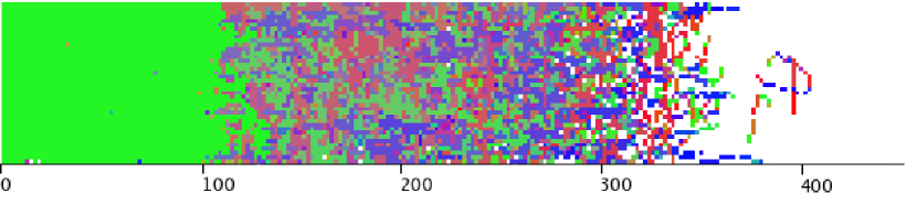
Figure 15: (Color online) (a) Profiles of the orientational order parameter, $S(z)$ (pluses $+$), and of the volume fraction of monomer units, $\phi(z)$ (crosses $\times$), for the $80\times 80\times 1000$ system, for the parameters $f=8.0$, $\varepsilon_{0}=0$, $N=20$, ${\cal N}=1600$, $\lambda_{g}=0.01$. Squares indicate the density values at coexistence, while the circles indicate the values of the nematic order parameter at coexistence. These values were extracted from the bulk grand canonical simulation (Fig. 12). The inset shows an enlarged region with the isotropic-nematic interface. (b) Two dimensional $xz$-map of the coarse–grained order parameter profile for a system snapshot corresponding to (a); for details of calculation see the text and Ref.LCpaper2, .

However, for the case $f=8.0$, $\varepsilon_{0}=0$ some problems of SE method start to appear because of the formation of a nematic phase formed on the hard wall. What happens in the system is shown in Fig. 15a where the profile of the orientational order parameter, $S(z)$, is plotted together with the density (volume fraction) profile, $\phi(z)$. The standard nematic order parameter tensor, Eq.(20), was calculated for bond vectors in each of the $xy$-layers along the $z$-axis separately and averaged over many conformations. Afterwards its maximal eigenvalue was calculated giving the orientational order parameter $S$ in each layer. The points indicated by squares and circles in Fig. 15a (and in the inset showing the transition regime in an enlarged scale) present the data for density (squares) and orientational order parameter (circles) in the isotropic (filled symbols) and in the nematic (open symbols) phases obtained from the grand canonical simulations at $\mu=-166$ (see Fig. 12) which exactly corresponds to the transition point. We used the values of the bulk densities to locate the layer $z$ where the same value of density occurs in the system with the wall, and then we plotted the value of $S$ in the bulk system at the same layer $z$. In Fig. 15b we present the two-dimensional $xz$-map of the coarse-grained order parameter profile for this system using red, green and blue colors to represent the average local orientation of monomer units along $x$, $y$ and $z$ axes, respectively (the details of the calculation method can be found in Ref.LCpaper2, ). From both these figures (Fig. 15a and 15b) one can see that the wall stabilizes rather thick domains of the nematically ordered phase.

One can observe a kink in the z-dependence of the density profile exactly between the two coexisting bulk densities of the isotropic-nematic transition. The order parameter, however, starts to rise significantly before the limiting isotropic density in the bulk is reached and has a value around $0.5$ at this density, whereas the corresponding bulk value is close to zero. The order parameter profile appears strongly rounded and slightly shifted with respect to the bulk simulations. These effects prevent an exact localization of the values of density and order parameter at the isotropic-nematic transition by the SE method. The rounding of the transition is unavoidable and mainly due to the presence of capillary wave excitations of the interfacerowl-widom , which would even increase in magnitude upon an increase of the lateral dimension of the simulation boxcapill01 ; capill02 , in contrast to the grand canonical bulk simulations where one can reduce finite size effects by increasing the system size. The slight shift of the transition in the order parameter profile as opposed to the density profile is an indication of a precursor of a nematic wetting layer at the hard wall.

It is interesting to compare the dependence of the orientational order parameter $S$ on the density $\phi$ (see Fig. 16) obtained by means of SE and TI$\mu VT$ methods which can be extracted from the data presented in Fig. 15a and Figs. 12a and 12c, respectively. Again, the TI$\mu VT$ data show a hysteresis while the SE data exhibit a smooth transition. It should be emphasized that both in the isotropic and nematic phases outside the hysteresis region the curves for both methods coincide with each other indicating that the SE method reproduces the properties of nematic phase correctly despite the vicinity of a hard wall.

The inevitable presence of the interface leads to a smoothing of the first order transition on the pressure vs. density dependence (Fig. 17a). In this Figure both the data for the SE method are presented using different values of $H$ and $\lambda_{g}$, as well as the data for the TI$\mu VT$ method which we have already discussed above. It is clear from the principle of the SE method that it is impossible to observe any hysteresis on the equation of state. Fig. 17a shows that the $\pi(\phi)$ curves generated by the SE method start to deviate from those generated by TI$\mu VT$ method near $\phi=0.28$, while for $\phi<0.28$ the agreement between both methods is excellent as well as for $\phi>0.36$ (these parts are not shown here). All curves for the SE method obtained at different values of $H$ and $\lambda_{g}$ almost coincide with each other (a variation of the lateral box linear dimension $L$ has no detectable effect on SE results) except for one data set shown with small filled squares ($H=500$, ${\cal N}=1600$, $\lambda_{g}=0.005$). In Figs. 17b the density profiles are presented and the reason for the deviation of the one data set becomes apparent: this is the only curve where the isotropic–nematic interface (which shows up as a characteristic kink in the density profile) appears very close to the hard wall (note that for $f=8.0$ the end-to-end distance of a chain is $R_{e}\approx 40$ (Fig. 8) and the chains are already rather stretched (Fig. 12b)) so that layering effects influence the isotropic–nematic coexistence in this case significantly. The effect of the layering at the wall, which can be quite strong (see Fig. 17b) on the equation of state in the isotropic regime decreases with increasing distance of the isotropic-nematic interface from the wall, such that the curves for the SE method in (Fig. 17a) already coincide within our error bars. Note also, that the ordinate of the kink in the density profiles in Fig. 17b is the same for all systems at different parameters. For the bulk simulation (the TI$\mu VT$ data) for different systems presented in Fig. 17a we can conclude that there exists an incommensurability effect which influences the equation of state: large open circles show the well equilibrated data obtained in the cubic box $L=90$, $H=90$ (box 1, see also above), and the hysteresis region is different from the one obtained for $L=80$, $H=150$ (box 2) shown with stars and large open squares.

Finally, we mention here a scaling of the density profiles shown in Fig. 18 (for details see the figure caption) which is also in agreement with results obtained in Ref.Hansen, . The curves superimpose for the systems where the combination of parameters ${\cal N}\lambda_{g}$ has the same value. The curves for larger values of ${\cal N}\lambda_{g}$ look broader and smoother in these scaled variables $\phi/({\cal N}\lambda_{g})$ vs. $z\lambda_{g}$ and show up the kink (isotropic–nematic interface) further away from the hard wall.

It is interesting to compare our conclusion on the shift of isotropic–nematic transition with the results of computer simulation studies of hard rod colloidal suspensions in confinements, i.e. solutions confined between hard walls and/or exposed to an external gravitational potential. A shift of the isotropic–nematic transition to lower densities as compared to the bulk was found for a hard-rod fluid confined by two wallsDijkstra03 . At the same time, a surprisingly good agreement between two osmotic equations of state for hard-rod fluids obtained from computer simulation using the SE method and from bulk simulations at many different densities has been reported in Ref.Dijkstra04, , also for densities in the nematic phase. The authors of Ref.Dijkstra04, explained this agreement by a very small interfacial width of the isotropic–nematic interface in comparison with the gravitational lengths considered in their work, a situation which is also realized in our simulations. However, for the model in Ref.Dijkstra04, the density difference between isotropic and nematic phase is very small and any possible deviations between the bulk equation of state and the results from the SE method simulations in the crossover density regime are not visible within the resolution and statistical uncertainty of the simulations.

Theoretically the effect of gravity on the phase behavior of hard rod solutions was studied in Ref.Baulin, . Comparing density and order parameter profiles in Figs. 15a with those calculated in Ref.Baulin, we can see a very good agreement: the density profiles show a quite small jump at the transition point and a smooth but significant decrease both in nematic and isotropic phases, while the orientational order parameter is almost constant within each of two phases and experiences a quite large jump at the transition point.

VI Conclusions

Monte Carlo computer simulations using the bond fluctuation model have been performed for solutions of semiflexible chains of the length $N=20$ monomer units. Three methods for pressure calculation in lattice Monte Carlo simulations have been investigated and compared: (1) the thermodynamic integration method in the grand canonical ensemble (TI$\mu VT$); (2) the repulsive wall method in the grand canonical ensemble (RWTI); (3) the sedimentation equilibrium method (SE) in the canonical ensemble in an external sedimentation field. All three methods show quite similar results for solutions of flexible chains as well as for the region of the isotropic phase of semiflexible chains. However, differences may occur at higher densities (or pressures) where for semiflexible chains the transition to the nematic phase takes place. Methodological problems of pressure measurement in solutions in the vicinity of isotropic-nematic transitions have been discussed.

The most crucial point is that the presence of a hard repulsive wall and/or an external sedimentation field exerts a significant influence on the isotropic-nematic transition, both on the transition point (transition density) and also on the structure of the ordered phase.

Thus we have found that the SE method is useful for obtaining the equation of state of various polymeric systems but its use becomes problematic in the vicinity of phase transitions. We have demonstrated this for the isotropic-nematic transition in solutions of semiflexible chains. The SE method works quite well sufficiently below and above the density of the isotropic-nematic transition, but it fails to predict the transition density correctly, at least for system sizes (which were reasonably large) and sedimentation field strengths (which were reasonably small) used in our simulations.

The source of the problems that we encountered is that for a system undergoing a transition from the isotropic to the nematic phase the SE method implies that for densities large enough that the nematic phase can develop in the simulation box, one necessarily must have a transition zone of densities where the nematic–isotropic interface is present in the box. This nematic–isotropic interface is not sharp but rather extended, and hence it is not clear from data such as Fig. 15 to judge where the region of the ”bulk” nematic phase stops and where the region of the interface begins. In fact, for an equilibrium interface in the absence of an external (gravitational) field we would have a smooth interfacial profile between the coexisting phases as well. This profile can be (at least approximately) considered as the convolution of an intrinsic profile with capillary–wave–induced broadening, which increases with the logarithm of the lateral system size, proportional to $\ln L$. Note, that already in this case the problem of disentangling the interfacial profile from the capillary wave broadening is notoriously difficult. However, in the presence of a gravitational field the problem is even more subtle: while strong gravitational fields will lead to a ”squeezing” of the intrinsic interface (similar to the squeezing of interfaces by very strong confinement), and eliminate the capillary wave broadening completely, weak gravitational fields will leave the intrinsic profile more or less intact, but eliminate the long wavelength part of the capillary wave spectrum. As a consequence, one expects a crossover from a broadening proportional to $\ln L$ for not too large $L$ to a finite width independent of $L$ but controlled by the strength of the gravitational field. An explicit study of all these interfacial phenomena is beyond the scope of the present paper. The problem gets even more complicated by the fact that also in the ”bulk” nematic phase the nematic order parameter is not at all constant, but varies with the distance $z$ from the wall, since the order parameter near the transition depends strongly on density, and thus a strong variation of order parameter is caused by the density variation as well. In view of these problems, it is difficult from the SE method to estimate accurately at which density the region of the isotropic phase stops and at which (higher) density then the region of the nematic phase begins. An estimation of the nematic order parameter at the transition point is hardly possible.

A particularly subtle difficulty occurs if parameters such as system size $H$ in the long direction and strength of the gravitational potential are chosen such, that there is not enough space left for the nematic phase to develop, and the isotropic–nematic interface occurs directly adjacent to the wall (Fig. 17b). Then data for the osmotic pressure in the transition region are obtained that are systematically too small, and suggest a transition from the isotropic to the nematic phase at a density that is clearly too low. This example shows that one must not rely on the SE method blindly when a phase transition occurs, but one needs then to check that the results are not changing when the strength of the gravitational field and/or the size in the long direction are varied.

We restricted ourselves to the chain length $N=20$ monomer units because in the bond-fluctuation model this chain length is sufficiently long to display Gaussian behavior in its chain statistics in the melt (i.e., it is a real flexible polymer, not an oligomer) and it is not too long to allow for a sufficiently efficient simulation. We should emphasize that the SE method is valid for polymer chains of any length, provided the length scale of variation of the external potential in which the sedimentation equilibrium is reached is much larger than the radius of gyration of a polymer chain, e.g., flexible chains of the length up to 500 monomer units have been studied in Ref.Hansen, . However, for the semiflexible chains the effect of chain stiffening in the nematic stateLCpaper1 will necessarily require much larger simulation boxes in comparison to the case of flexible chains of the same length.

While the TI$\mu VT$ method near the isotropic–nematic transition is hampered by hysteresis, Fig. 12, the fact that the transition in the $(\pi,\mu)$ plane must show up as a simple intersection point of the curves does allow an accurate location of the transition (Fig. 13a), and to characterize the magnitudes of the jumps. In this way, the strictly horizontal part in the $\pi$ vs. $\phi$ isotherm (Fig. 13b) can be constructed. Thus, we feel that for the accurate characterization of first order phase transitions the TI$\mu VT$ method is preferable, whenever applicable. With respect to the numerical data presented in this paper, we add the caveat that there may be still some systematic errors due to a too small value chosen for the lateral size $L$. However, the same size was used for the simulations by means of SE method, and hence we think that our discussion of the relative merits of these methods should not be affected by this problem.

In future work, we plan to extend these studies to include also attractive interaction between the monomer units, to investigate the competition between nematic ordering and polymer–solvent phase separation, applying the methods validated in the present paper.

Figure 1: Osmotic pressure $\pi$ plotted vs. polymer volume fraction $\phi$, for the athermal fully flexible bond fluctuation model on the simple cubic lattice. The solid line shows the TI$\mu VT$ results, while the two large squares indicate results obtained with the RWTI method. Filled circles are the corresponding RWTI results of Deutsch and Dickman (Ref. rep_wall2, ).

Figure 2: Difference between osmotic pressure $\pi$ obtained with the TI$\mu VT$ and SE methods plotted vs. $\phi$. Note that the difference is less than $10^{-3}$ throughout and almost no systematic trend can be seen (see also discussion in Section V below). The SE data were obtained for a system of size $80\times 80\times 200$ containing ${\cal N}=1600$ chains, for a choice of $\lambda_{g}=0.01$.

a)

b)

Figure 3: (a) Osmotic pressure $\pi$ (on a logarithmic scale) plotted vs. volume fraction $\phi$ (on a logarithmic scale), for the fully athermal solution of flexible chains of length $N=20$, comparing several variants of the SE method for a box of size $80\times 80\times 250$ and ${\cal N}=1200$. Open squares refer to the gravitation–like potential, Eq. (6), with $\lambda_{g}=0.01$, while the filled circles and stars refer to the potential in Eq. (12) with $\kappa=1/2$, using $\lambda_{g}^{\prime}=0.1$ and 0.5 correspondingly. The full line is the exactly known ideal gas limit. (b) Density (volume fraction) profiles of monomer units, $\phi(z)=2n_{m}(z)/n_{max}$, corresponding to the results shown in (a); solid line is for gravitation-like potential with $\lambda_{g}=0.01$, dashed-dotted line is for $\lambda_{g}^{\prime}=0.5$, $\kappa=1/2$, and dotted line is for $\lambda_{g}^{\prime}=0.1$, $\kappa=1/2$; here $n_{m}(z)$ is the average number of monomer units at the altitude $z$, $n_{max}=L^{2}/4$ is the maximal number of monomers in one layer, and the coefficient 2 in the formulae for $\phi(z)$ above accounts for the fact that one fully occupied layer excludes for occupation all lattice sites in a neighboring layer. Note that the density profile for the case $\lambda_{g}^{\prime}=0.1$ is affected by the wall at $z=250$ (the inset shows the same figure using a logarithmic scale for the density), leading to systematic errors in the equation of state. The decay of density profiles always occurs on scales much larger than the average value of gyration radius $\sqrt{\langle R_{g}^{2}\rangle}$ which was about $6.4$ for dilute region and about $5.6$ in the concentrated region close to the wall.

a)

b)

Figure 4: (a) Same as Fig. 3a, but comparing the results for the gravitation-like potential, Eq. (6), with $\lambda_{g}=0.01$ (filled circles) to results for the potential in Eq. (12) with $\kappa=2$, using $\lambda_{g}^{\prime}=0.0001$ (open squares) and $\lambda_{g}^{\prime}=0.001$ (stars). (b) Density (volume fraction) profiles of monomer units corresponding to the results shown in Fig. 4a; solid line is for gravitation-like potential with $\lambda_{g}=0.01$, dashed-dotted line is for $\lambda_{g}^{\prime}=0.001$, $\kappa=2$, and dotted line is for $\lambda_{g}^{\prime}=0.0001$, $\kappa=2$.

Figure 5: Semi-log plot of the density profiles of monomer units for three choices of the external potential: Eq. (6) with $\lambda_{g}=0.01$ (stars) with the asymptotic barometric law (solid line), Eq. (12) with $\kappa=1/2$, $\lambda_{g}^{\prime}=0.5$ (filled circles) with the corresponding asymptotic law (dashed-dotted line) and with $\kappa=2$, $\lambda_{g}^{\prime}=0.0001$ (open squares) with the asymptotic law (dashed line). For all cases the box size was $80\times 80\times 250$ and the number of chains was ${\cal N}=1200$.

a)

b)

Figure 6: Chemical potential per chain vs. volume fraction $\phi$, for the case of fully flexible chains, (a), where both $f=0$ and $\varepsilon_{0}=0$, and for semiflexible ones, (b), with $f=2.68$, $\varepsilon_{0}=4$. Note the logarithmic scale of the abscissa. Straight solid line indicates the fit to Eq. (19), with $C(0,0)=-82.5$ and $C(2.68,4)=38.0$, respectively.

a)

b)

Figure 7: Bending energy per chain (a) and $C(f,0)$ (b) plotted vs. the stiffness parameter $f$. Thin solid line in (a) indicates the linear fit. In part (b) $C(f,0)$ is plotted with stars ($*$) and solid line, while symbols indicate approximations where $C(f,0)$ is found from a decomposition of the chain partition function in terms of independent trimers (open squares), tetramers (open circles) and pentamers (filled circles).

a)

b)

Figure 8: Mean squared end-to-end distance (a) and mean squared gyration radius (b) plotted vs. volume fraction $\phi$, for several choices of the stiffness parameter $f$, $f=0$ (filled triangles), $f=1.2$ (open squares), $f=2.68$ (filled squares), $f=4$ (open circles), $f=8$ (filled circles), $f=20$ (open triangles), and $\varepsilon_{0}=0$.

a)

b)

Figure 9: Equation of state $\pi(\phi)$ plotted vs. $\phi$, for several choices of the stiffness parameter $f$ and two choices for the bond length energy parameter $\varepsilon_{0}$ (a). Magnified view of the equation of state in the low density regime (b); the ideal gas limit $\pi=\phi/160$ is indicated by a thin solid line. The choices of the parameter $f$ (and $\varepsilon_{0}$ in part (a); part (b) refers to $\varepsilon_{0}=0$ only) are given in the figure. Curves are obtained using the TI$\mu VT$ method.

a)

b)

Figure 10: Osmotic pressure $\pi$ plotted vs. the chemical potential $\mu$ (a) and versus the volume fraction $\phi$ (b), for the model with parameters $f=2.68$ and $\varepsilon_{0}=4$. Curves are obtained using the TI$\mu VT$ method (filled triangles correspond to a dense packed starting conformation, while open squares to a dilute isotropic one), the two large open circles show results obtained from the RWTI method. The inset shows an enlarged region in the vicinity of the isotropic–nematic transition.

Figure 11: Density (volume fraction) profile of a $60\times 60\times 180$ system (only half of the symmetric profile is shown) for the parameters $f=2.68$ and $\varepsilon_{0}=4$ at $\phi\approx 0.34$, as used for the calculation of the pressure $\pi(\phi)$ in the RWTI method. Different curves for different values of the repulsion parameter $\lambda$ from $\lambda=0.02$ to $\lambda=1.0$ are superimposed.

a)

b)

c)

Figure 12: Hysteresis for the density vs. $\mu$ dependence (a), for the dependence of the single-chain orientational order parameter, $S_{chain}$, vs. $\mu$ (b) and the total orientational order parameter, $S$, vs. $\mu$ (c). Filled triangles correspond to a dense packed starting conformation, while open squares correspond to a dilute isotropic starting conformation. In part (c) for the case of a dilute isotropic starting conformation only data points for $\mu$ below the jump to a nematic state are presented. Vertical lines show the estimated value of the chemical potential at the transition point, $\mu=-166\pm 0.5$ (determined in Fig. 13).

a)

b)

Figure 13: (a) The dependence of the pressure vs. chemical potential for $f=8$, $\varepsilon_{0}=0$, obtained by TI$\mu VT$ method; the inset shows the difference $\pi_{nematic}-\pi_{isotropic}$ in the region close to the isotropic-nematic transition on enlarged scales. Filled triangles correspond to a dense packed starting conformation, while open squares to a dilute isotropic one. (b) The equation of state for $f=8$, $\varepsilon_{0}=0$ (solid and dotted lines). The hysteresis region as well as determined transition line are well visible. Two open squares indicate densities in the coexisting phases.

a)

b)

Figure 14: (a) Equation of state $\pi(\phi)$ for an athermal solution of semiflexible chains, with the parameters of the bending energy {Eq. (15)} chosen as $\varepsilon_{0}=0$ and $f=4$ (a). Open circles are the results of the TI$\mu VT$ method, while the solid line is the result of the SE method, choosing the potential Eq. (6) and $\lambda_{g}=0.01$. The box size was equal to $80\times 80\times 250$, the number of chains was equal to ${\cal N}=1600$. Part (b) shows the density profile for the SE method. The inset shows an enlarged region in the vicinity of the wall where the layering is well visible.

a)

b)

Figure 16: Dependence of the nematic orientational order parameter $S$ on the density $\phi$: comparison of TI$\mu VT$ data (open and filled triangles) with SE data (solid line). The two large open circles indicate the isotropic–nematic transition.

a)

b)

Figure 17: (a) Equation of state $\pi(\phi)$ for the case $f=8.0$, $\varepsilon_{0}=0$, $N=20$, $L=80$ using the SE method for several choices of ${\cal N}$, $H$ and $\lambda_{g}$ as indicated in the legend: $\lambda_{g}=0.01$, $H=250$, ${\cal N}=1600$ (small open squares); $\lambda_{g}=0.005$, $H=500$, ${\cal N}=1600$ (small filled squares); $\lambda_{g}=0.005$, $H=1000$, ${\cal N}=3200$ (small open circles); $\lambda_{g}=0.007$, $H=500$, ${\cal N}=1600$ (small filled triangles). Additionally, large open circles (and the solid line which is only a guide for the eye) show the result of the TI$\mu VT$ method for the box $90\times 90\times 90$. Stars and dashed lines (as a guide for the eye) are the results of the TI$\mu VT$ simulations in the box $80\times 80\times 150$ (from Fig. 13b). The isotropic–nematic transition line is visible between two large open squares indicating the coexisting densities. Regions of the density profiles with a kink indicating the isotropic–nematic transition are presented in (b) for $\lambda_{g}=0.005$ and different $H$ and ${\cal N}$ as indicated in the legend.

Figure 18: Rescaled density profiles $\phi/({\cal N}\lambda_{g})$ vs. $z\lambda_{g}$ for several systems, as indicated in the legend. Note that curves with the same value of ${\cal N}\lambda_{g}$ practically superimpose. The average value of the gyration radius $\sqrt{\langle R_{g}^{2}\rangle}$ is about $14.8$ both in the dilute and concentrated regions.

References

- (1) P. J. Flory, Principles of Polymer Chemistry (Cornell University Press, Ithaca, 1953).
- (2) P. G. de Gennes, Scaling Concepts in Polymer Physics (Cornell University Press, Ithaca, 1979).
- (3) J. de Cloizeaux and G. Jannink, Polymers in Solution: Their Modelling and Structure (Clarendon Press, Oxford, 1990).
- (4) A. Yu. Grosberg, A. R. Khokhlov, Statistical Physics of Macromolecules (AIP Press, New York, 1994).
- (5) K. Binder (ed.) Monte Carlo and Molecular Dynamics Simulations in Polymer Science (Oxford University Press, New York, 1995).
- (6) L. Schäfer, Excluded Volume Effects in Polymer Solutions (Springer-Verlag, Berlin, 1999).
- (7) M. Rubinstein, R. H. Colby, Polymer Physics (Oxford University Press, Oxford, 2003).
- (8) A. R. Khokhlov and A. N. Semenov, J. Stat. Phys. 38, 161 (1985); Macromolecules 19, 373 (1986).
- (9) See e.g. V. A. Ivanov, W. Paul, K. Binder, J. Chem. Phys. 109, 5659 (1998); J. A. Martemyanova, M. R. Stukan, V. .A Ivanov, M. Müller, W. Paul, K. Binder, J. Chem. Phys. 122, 174907 (2005), and references therein.
- (10) M. J. Kotelyanskii and D. N. Theodorou (eds.) Simulation Methods for Polymers (M. Debber, New York, 2004).
- (11) G. Strobl, The Physics of Polymers (Springer, Berlin, 1996).
- (12) B. Widom, J.Stat.Phys. 52, 1343 (1988).
- (13) N. Wilding, M. Müller, K. Binder, J.Chem.Phys. 105, 802 (1996).
- (14) K. Binder, M. Müller, P. Virnau and L. G. MacDowell, Adv.Polym.Sci. 173, 1 (2005), and references therein.
- (15) P. J. Flory, Proc. Roy. Soc. London A234, 60 (1956); ibid. A234, 73 (1956); T. Odijk, Macromolecules 19, 2313 (1986); A. N. Semenov and A. R. Khokhlov, Sov. Phys. Uspekhi 31, 988 (1986).
- (16) A. Baumgärtner, J. Chem. Phys, 84, 1905 (1986); A. Kolinsky, J. Skolnick and R. Yaris, Macromolecules 19, 2560 (1986); M. R. Wilson and M. R. Allen, Mol. Phys. 80, 277 (1993); M. Dijkstra and D. Frenkel, Phys. Rev. E 51, 5891 (1995).
- (17) H. Weber, W. Paul, K. Binder, Phys. Rev. E 59, 2168 (1999).
- (18) H. H. Strey, V. A. Parsegian, and R. Podgornik, Phys. Rev. E 59, 999 (1999).
- (19) C. Vega, C. McBride and L. G. MacDowell, J. Chem. Phys. 115, 4203 (2001); C. McBride, C. Vega and L. G. MacDowell, Phys. Rev. E 64, 011703 (2001); C. Vega, C. McBride and L. G. MacDowell, Phys. Chem. Chem. Phys. 4, 853 (2002); C. McBride and C. Vega, J. Chem. Phys. 117, 10370 (2002).
- (20) A. R. Khokhlov, Polym. Sci. USSR 21, 2185 (1979); A. Yu. Grosberg and A. R. Khokhlov, Adv. Polym. Sci. 41, 53 (1981).
- (21) V.A.Ivanov, M.R.Stukan, M.Müller, W.Paul, K.Binder, J.Chem.Phys. 118, 10333 (2003).
- (22) M.R.Stukan, V.A.Ivanov, M.Müller, W.Paul, K.Binder, ePolymers no.062 (2003); http://www.e-polymers.org.
- (23) M. P. Allen and D. J. Tildesley, Computer Simulation of Liquids (Clarendon Press, Oxford, 1987).
- (24) A. Bellemans and E. De Vos, J. Polym. Sci. Symp. 42, 1195 (1973); H. Okamoto, J.Chem. Phys. 64, 2686 (1976); H. Okamoto, J. Chem. Phys. 79, 3976 (1983); ibid. 83, 2587 (1985).
- (25) R. Dickman, C. K. Hall, J. Chem. Phys. 85, 3023 (1986).
- (26) D. Frenkel and B. Smit, Undestanding Molecular Simulation. From Algorithms to Applications. 2nd Edition (Academic Press, New York, 2002).
- (27) D. P. Landau and K. Binder, A Guide to Monte Carlo Simulation is Statistical Physics (Cambridge University Press, Cambridge, 2005).
- (28) J. I. Siepmann, Mol. Phys. 70, 1145 (1990); G. C. A. M. Mooij and D. Frenkel, Mol. Phys. 74, 41 (1991); J. I. Siepmann and D. Frenkel, Mol. Phys. 75, 59 (1992); D. Frenkel and B. Smit, Mol. Phys. 75, 983 (1992).
- (29) M. Müller, W. Paul, J. Chem. Phys. 100, 719 (1994).
- (30) R. Dickman, J. Chem. Phys. 87, 2246 (1987); R. Dickman, C. K. Hall, J. Chem. Phys. 89, 3168 (1988); A. Hertanto, R. Dickman, J. Chem. Phys. 89, 7577 (1988); R. Dickman, J. Chem. Phys. 91, 454 (1989).
- (31) H.-P. Deutsch, R. Dickman, J. Chem. Phys. 93, 8983 (1990).
- (32) M. R. Stukan, V. A. Ivanov, M. Müller, W. Paul, K. Binder, J. Chem. Phys. 117, 9934 (2002).
- (33) C. I. Addison, J.-P. Hansen, A. A. Louis, ChemPhysChem 6, 1760 (2005).
- (34) T. Biben, J.-P. Hansen, J.-L. Barrat, J. Chem. Phys. 98, 7330 (1993); R. Piazza, T. Bellini, V. Degiorgio, Phys. Rev. Lett. 71, 4267 (1993).
- (35) S. V. Savenko and M. Dijkstra, Phys. Rev. E 70, 051401 (2004).
- (36) M. Dijkstra, J.-P. Hansen, P. A. Madden, Phys. Rev. E 55, 3044 (1997).
- (37) J.-P. Hansen, C. I. Addison, A. A. Louis, J. Phys.: Condens. Matter 17, S3185 (2005).
- (38) C. I. Addison, J.-P. Hansen, V. Krakoviak, A. A. Louis, Mol. Phys. 103, 3045 (2005).
- (39) C. I. Addison, P.-A. Artola, J.-P. Hansen, A. A. Louis, J. Phys. Chem. B 110, 3661 (2006).
- (40) P. C. Hohenberg, M. Barmatz, Phys. Rev. A 6, 289 (1972).
- (41) M. Dijkstra, R. van Roij, R. Evans, Phys. Rev. E 63, 051703 (2001); R. van Roij, M. Dijkstra and R. Evans, Europhys. Lett. 49, 350 (2000).
- (42) I. Carmesin, K. Kremer, Macromolecules 21, 2819 (1988); H.-P. Deutsch and K. Binder, J. Chem. Phys. 94, 2294 (1990).
- (43) K. Binder, J. Baschnagel and W. Paul, Progr. Polym. Sci. 28, 115 (2003).
- (44) W. Paul, N. Pistoor, Macromolecules 27, 1249 (1994).
- (45) V. Tries, W. Paul, J. Baschnagel, and K. Binder, J. Chem. Phys. 106, 738 (1997).
- (46) J. S. Rowlinson, B. Widom, Molecular Theory of Capillarity (Clarendon Press, Oxford, 1982)
- (47) A. Werner, F. Schmid, M. Müller, and K. Binder, J. Chem. Phys. 107, 8175 (1997).
- (48) A. Werner, F. Schmid, M. Müller, and K. Binder, Phys. Rev. E 59, 728 (1999).
- (49) V. A. Baulin and A. R. Khokhlov, Phys. Rev. E 60, 2973 (1999).
a)
b)
a)
b)
a)
b)
a)
b)
a)
b)
a)
b)
a)
b)
a)
b)
c)
a)
b)
a)
b)
a)
b)
a)
b)